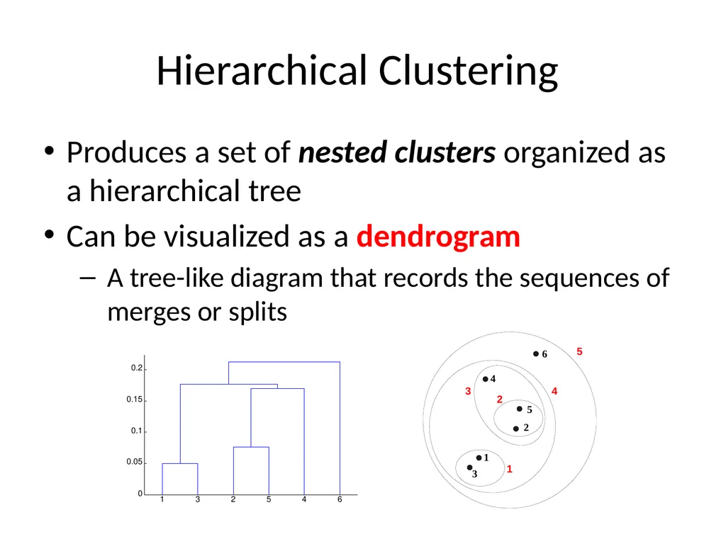
03
Strengths of Hierarchical Clustering No assumptions on the number of clusters
Any desired number of clusters can be obtained by ‘cutting’ the dendogram at the proper level
Hierarchical clusterings may correspond to meaningful taxonomies
Example in biological sciences (e.g., phylogeny reconstruction, etc), web (e.g., product catalogs) etc<br>
04
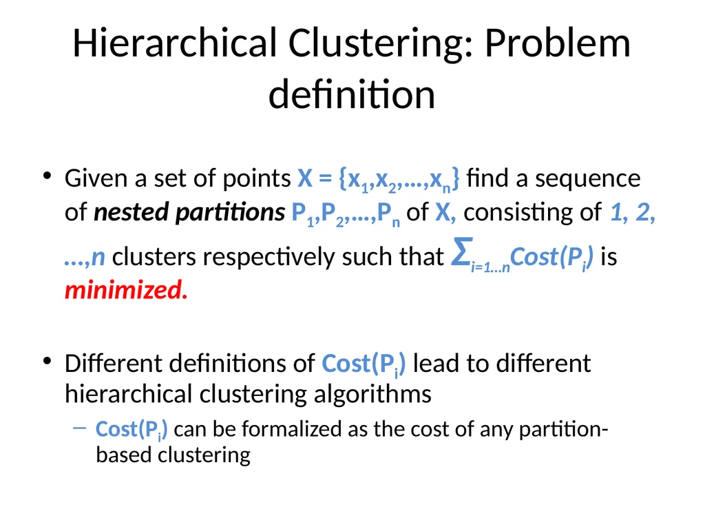
Hierarchical Clustering: Problem definition Given a set of points X = {x1,x2,…,xn} find a sequence of nested partitions P1,P2,…,Pn of X, consisting of 1, 2,…,n clusters respectively such that Σi=1…nCost(Pi) is minimized.
Different definitions of Cost(Pi) lead to different hierarchical clustering algorithms
Cost(Pi) can be formalized as the cost of any partition-based clustering<br>
05
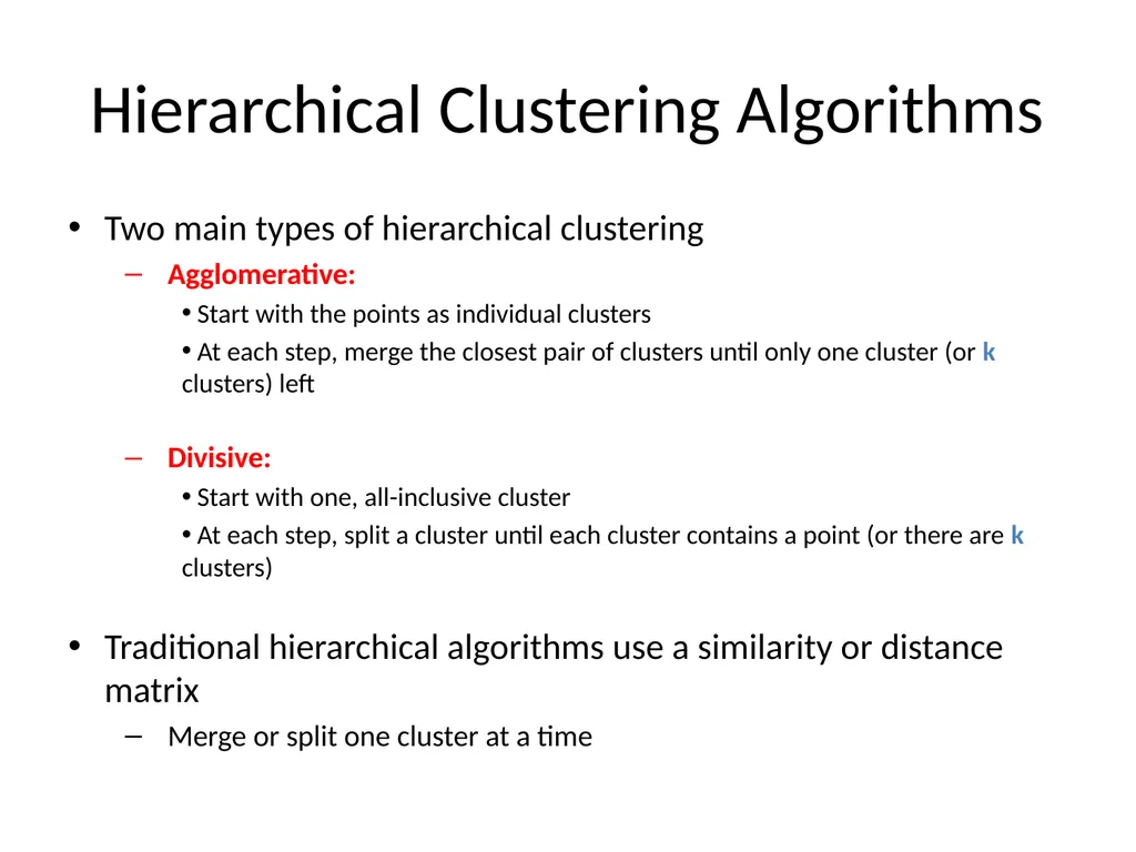
Hierarchical Clustering Algorithms Two main types of hierarchical clustering
Agglomerative:
Start with the points as individual clusters
At each step, merge the closest pair of clusters until only one cluster (or k clusters) left
Divisive:
Start with one, all-inclusive cluster
At each step, split a cluster until each cluster contains a point (or there are k clusters)
Traditional hierarchical algorithms use a similarity or distance matrix
Merge or split one cluster at a time<br>
06
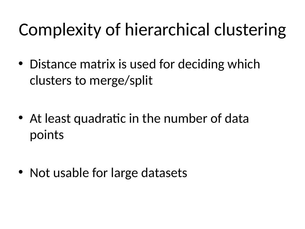
Complexity of hierarchical clustering Distance matrix is used for deciding which clusters to merge/split
At least quadratic in the number of data points
Not usable for large datasets<br>
07
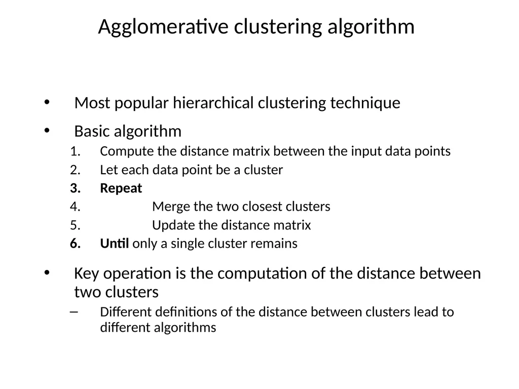
Agglomerative clustering algorithm Most popular hierarchical clustering technique
Basic algorithm
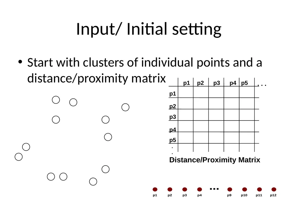
Compute the distance matrix between the input data points
Let each data point be a cluster
Repeat
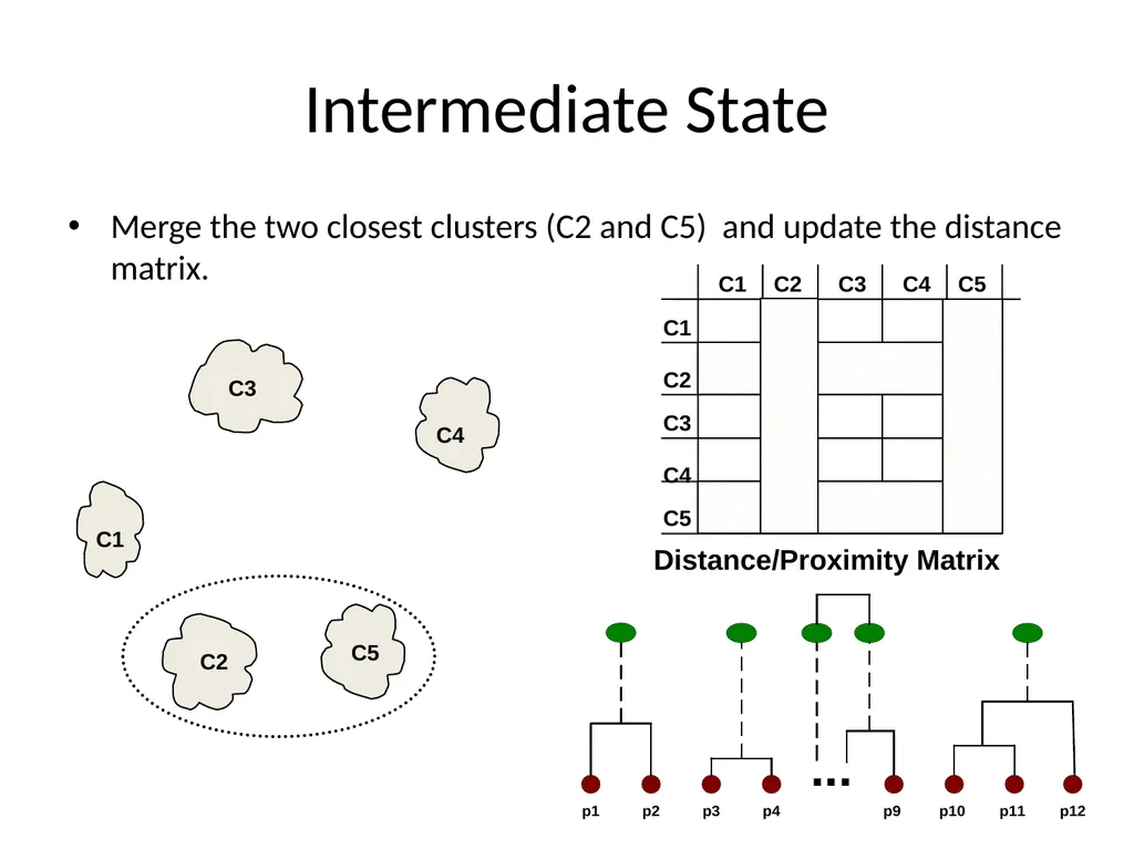
Merge the two closest clusters
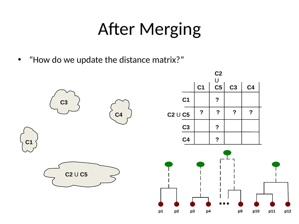
Update the distance matrix
Until only a single cluster remains
Key operation is the computation of the distance between two clusters
Different definitions of the distance between clusters lead to different algorithms<br>
08
Input/ Initial setting Start with clusters of individual points and a distance/proximity matrix Distance/Proximity Matrix<br>
09
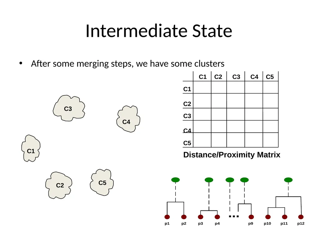
Intermediate State After some merging steps, we have some clusters C1 C4 C2 C5 C3 Distance/Proximity Matrix<br>
10
Intermediate State Merge the two closest clusters (C2 and C5) and update the distance matrix. C1 C4 C2 C5 C3 Distance/Proximity Matrix<br>
11
After Merging “How do we update the distance matrix?” C1 C4 C2 U C5 C3 ? ? ? ? ? ? ? C2 U C5 C1 C1 C3 C4 C2 U C5 C3 C4<br>
12
Distance between two clusters Each cluster is a set of points
How do we define distance between two sets of points
Lots of alternatives
Not an easy task<br>
13
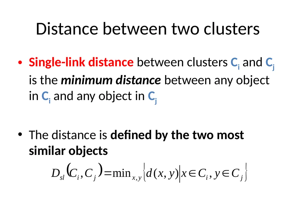
Distance between two clusters Single-link distance between clusters Ci and Cj is the minimum distance between any object in Ci and any object in Cj
The distance is defined by the two most similar objects<br>
14
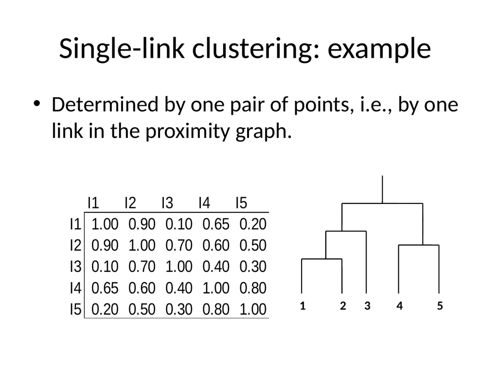
Single-link clustering: example Determined by one pair of points, i.e., by one link in the proximity graph.<br>
15
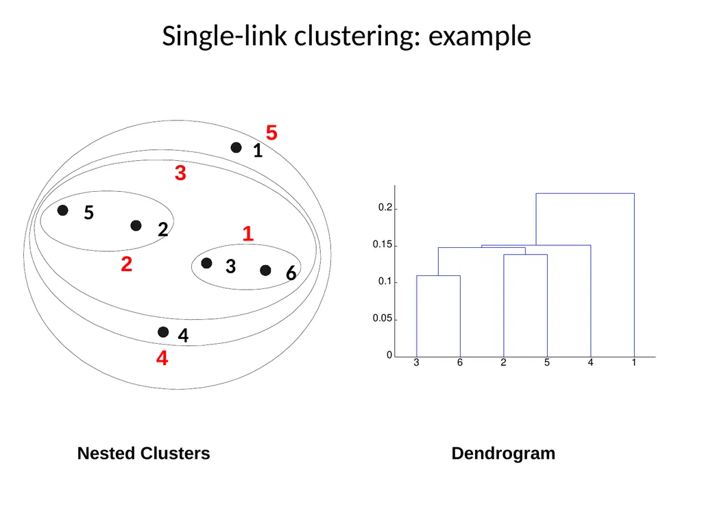
Single-link clustering: example Nested Clusters Dendrogram<br>
16
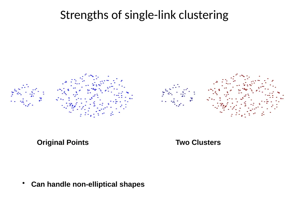
Strengths of single-link clustering Original Points Can handle non-elliptical shapes<br>
17
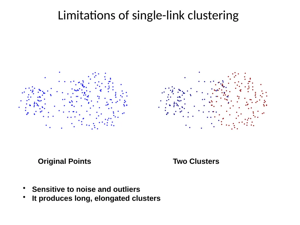
Limitations of single-link clustering Original Points Sensitive to noise and outliers
It produces long, elongated clusters<br>
18
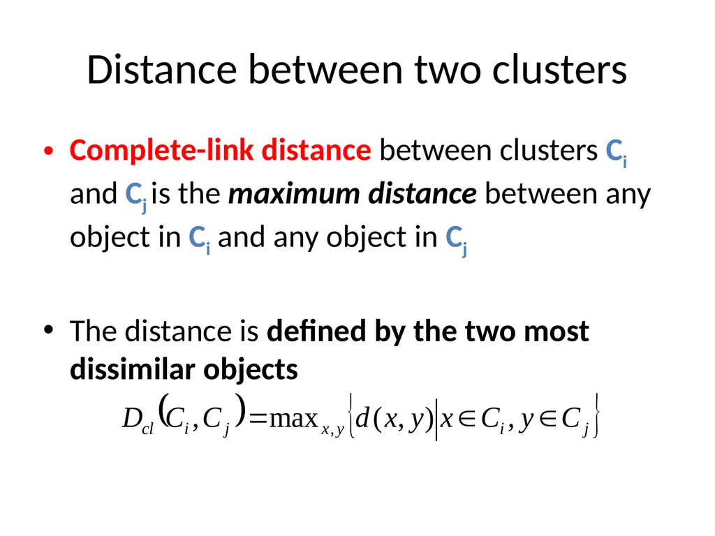
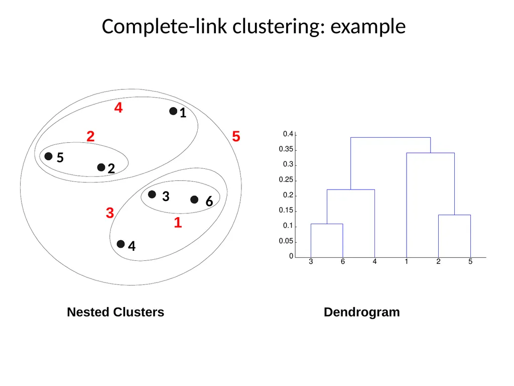
Distance between two clusters Complete-link distance between clusters Ci and Cj is the maximum distance between any object in Ci and any object in Cj
The distance is defined by the two most dissimilar objects<br>
19
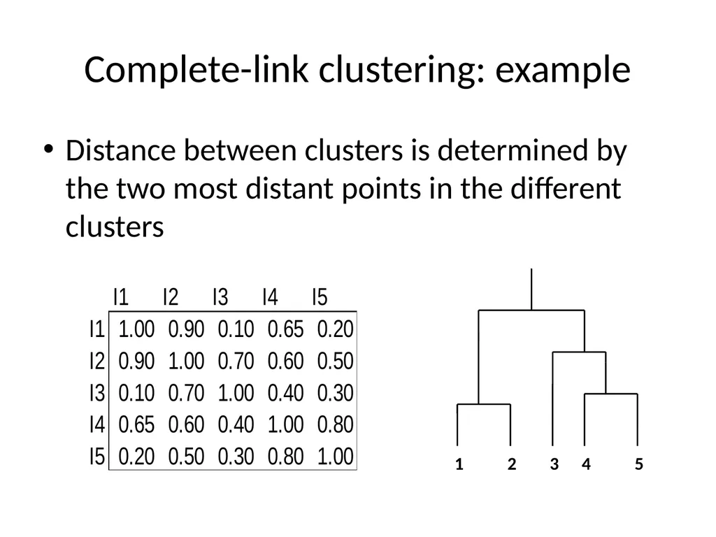
Complete-link clustering: example Distance between clusters is determined by the two most distant points in the different clusters<br>
20
Complete-link clustering: example Nested Clusters Dendrogram<br>
21
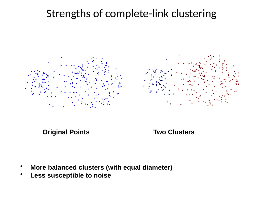
Strengths of complete-link clustering Original Points More balanced clusters (with equal diameter)
Less susceptible to noise<br>
22
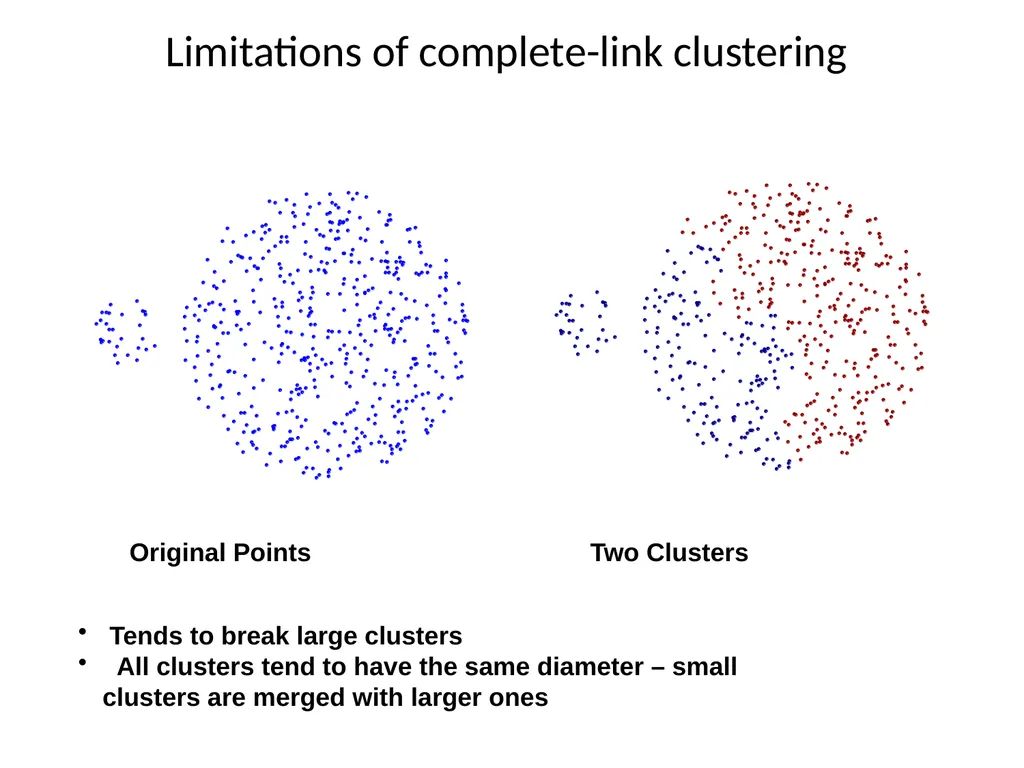
Limitations of complete-link clustering Original Points Tends to break large clusters
All clusters tend to have the same diameter – small clusters are merged with larger ones<br>
23
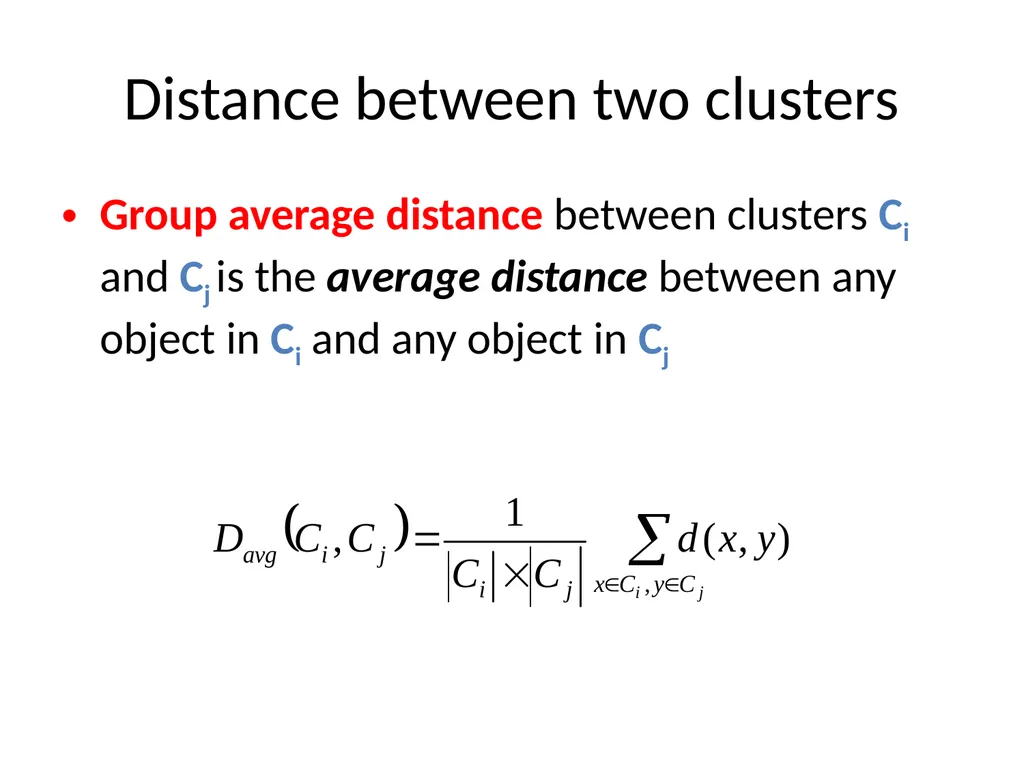
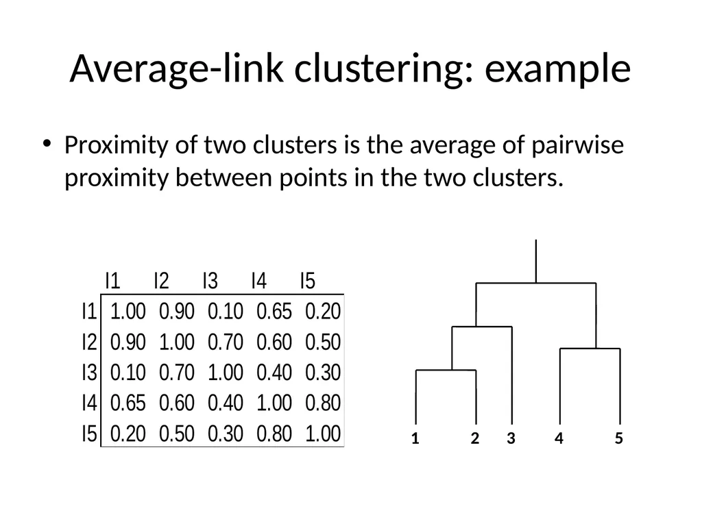
Distance between two clusters Group average distance between clusters Ci and Cj is the average distance between any object in Ci and any object in Cj<br>
24
Average-link clustering: example Proximity of two clusters is the average of pairwise proximity between points in the two clusters.<br>
25
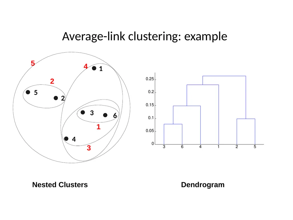
Average-link clustering: example Nested Clusters Dendrogram<br>
26
Average-link clustering: discussion Compromise between Single and Complete Link
Strengths
Less susceptible to noise and outliers
Limitations
Biased towards globular clusters<br>
27
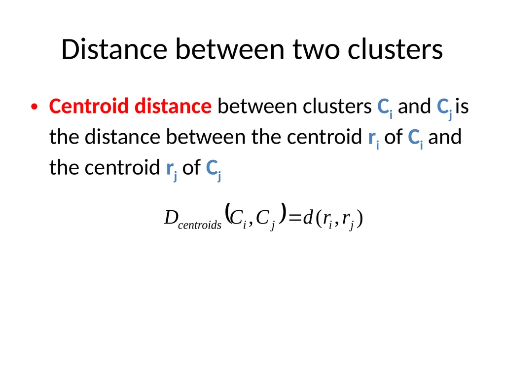
Distance between two clusters Centroid distance between clusters Ci and Cj is the distance between the centroid ri of Ci and the centroid rj of Cj<br>
28
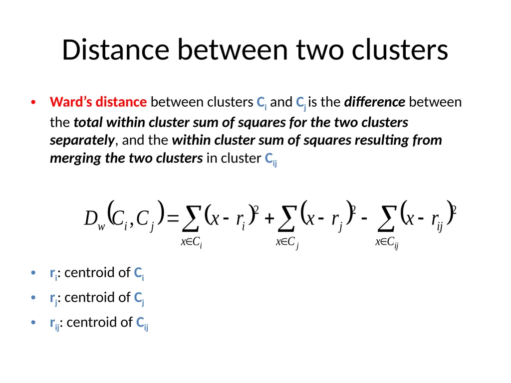
Distance between two clusters Ward’s distance between clusters Ci and Cj is the difference between the total within cluster sum of squares for the two clusters separately, and the within cluster sum of squares resulting from merging the two clusters in cluster Cij
ri: centroid of Ci
rj: centroid of Cj
rij: centroid of Cij<br>
29
Ward’s distance for clusters Similar to group average and centroid distance
Less susceptible to noise and outliers
Biased towards globular clusters
Hierarchical analogue of k-means
Can be used to initialize k-means<br>
30
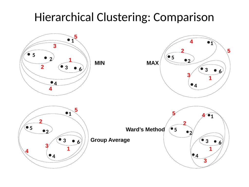
Hierarchical Clustering: Comparison Group Average Ward’s Method MIN MAX<br>
31
Hierarchical Clustering: Time and Space requirements For a dataset X consisting of n points
O(n2) space; it requires storing the distance matrix
O(n3) time in most of the cases
There are n steps and at each step the size n2 distance matrix must be updated and searched
Complexity can be reduced to O(n2 log(n) ) time for some approaches by using appropriate data structures<br>
32
Divisive hierarchical clustering Start with a single cluster composed of all data points
Split this into components
Continue recursively
Computationally intensive, less widely used than agglomerative methods<br>