
Highline Class, BI 348 Basic Business Analytics
DJ
Published · 48 slides · 0 views
1 / 1
Description
Highline Class, BI 348 Basic Business Analytics using Excel Chapter 05: Introduction to Basic Time Series Analysis and Forecasting 1 Topics Covered: Terms: Time Series and Forecast Time Series Patterns Basic Forecasting Methods: Most Recent
Related Topics
Share
Embed code
Download this presentation From Below
"Highline Class, BI 348 Basic Business Analytics" is the property of its rightful owner. Permission is granted to download and print the materials on this website for personal, non-commercial use only, and to display it on your personal computer provided you do not modify the materials and that you retain all copyright notices contained in the materials. By downloading content from our website, you accept the terms of this agreement.
Presentation Transcript
01
Highline Class, BI 348 Basic Business Analytics using Excel
Chapter 05: Introduction to
Basic Time Series Analysis and Forecasting 1<br>
Chapter 05: Introduction to
Basic Time Series Analysis and Forecasting 1<br>
02
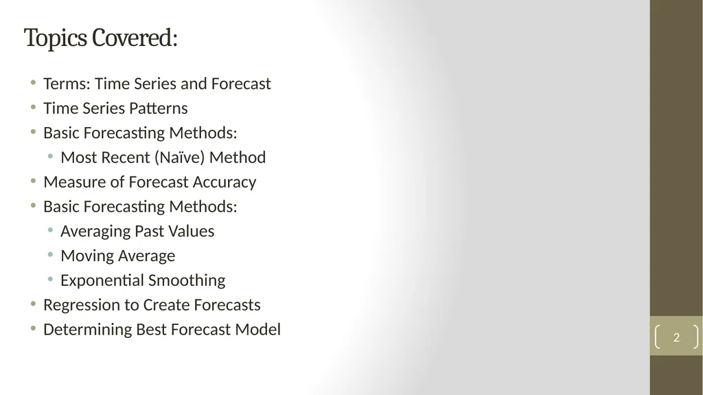
Topics Covered: Terms: Time Series and Forecast
Time Series Patterns
Basic Forecasting Methods:
Most Recent (Naïve) Method
Measure of Forecast Accuracy
Basic Forecasting Methods:
Averaging Past Values
Moving Average
Exponential Smoothing
Regression to Create Forecasts
Determining Best Forecast Model 2<br>
Time Series Patterns
Basic Forecasting Methods:
Most Recent (Naïve) Method
Measure of Forecast Accuracy
Basic Forecasting Methods:
Averaging Past Values
Moving Average
Exponential Smoothing
Regression to Create Forecasts
Determining Best Forecast Model 2<br>
03
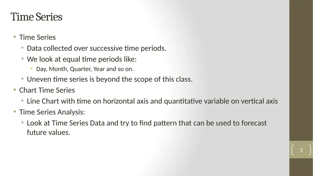
Time Series Time Series
Data collected over successive time periods.
We look at equal time periods like:
Day, Month, Quarter, Year and so on.
Uneven time series is beyond the scope of this class.
Chart Time Series
Line Chart with time on horizontal axis and quantitative variable on vertical axis
Time Series Analysis:
Look at Time Series Data and try to find pattern that can be used to forecast future values. 3<br>
Data collected over successive time periods.
We look at equal time periods like:
Day, Month, Quarter, Year and so on.
Uneven time series is beyond the scope of this class.
Chart Time Series
Line Chart with time on horizontal axis and quantitative variable on vertical axis
Time Series Analysis:
Look at Time Series Data and try to find pattern that can be used to forecast future values. 3<br>
04
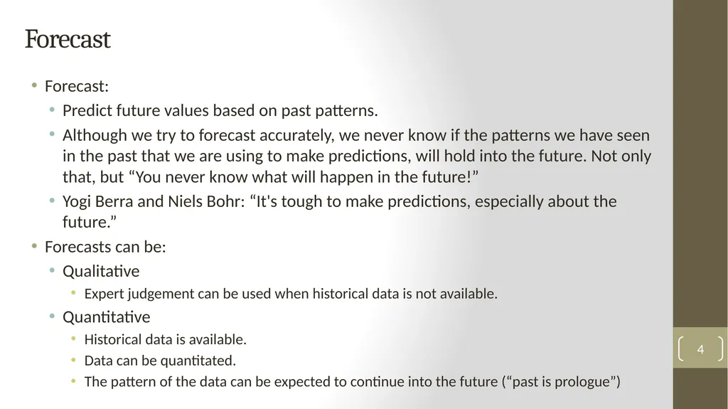
Forecast Forecast:
Predict future values based on past patterns.
Although we try to forecast accurately, we never know if the patterns we have seen in the past that we are using to make predictions, will hold into the future. Not only that, but “You never know what will happen in the future!”
Yogi Berra and Niels Bohr: “It's tough to make predictions, especially about the future.”
Forecasts can be:
Qualitative
Expert judgement can be used when historical data is not available.
Quantitative
Historical data is available.
Data can be quantitated.
The pattern of the data can be expected to continue into the future (“past is prologue”) 4<br>
Predict future values based on past patterns.
Although we try to forecast accurately, we never know if the patterns we have seen in the past that we are using to make predictions, will hold into the future. Not only that, but “You never know what will happen in the future!”
Yogi Berra and Niels Bohr: “It's tough to make predictions, especially about the future.”
Forecasts can be:
Qualitative
Expert judgement can be used when historical data is not available.
Quantitative
Historical data is available.
Data can be quantitated.
The pattern of the data can be expected to continue into the future (“past is prologue”) 4<br>
05
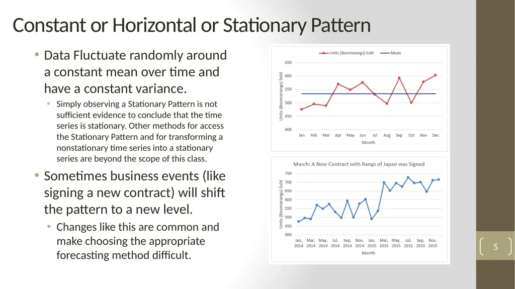
Constant or Horizontal or Stationary Pattern Data Fluctuate randomly around a constant mean over time and have a constant variance.
Simply observing a Stationary Pattern is not sufficient evidence to conclude that the time series is stationary. Other methods for access the Stationary Pattern and for transforming a nonstationary time series into a stationary series are beyond the scope of this class.
Sometimes business events (like signing a new contract) will shift the pattern to a new level.
Changes like this are common and make choosing the appropriate forecasting method difficult. 5<br>
Simply observing a Stationary Pattern is not sufficient evidence to conclude that the time series is stationary. Other methods for access the Stationary Pattern and for transforming a nonstationary time series into a stationary series are beyond the scope of this class.
Sometimes business events (like signing a new contract) will shift the pattern to a new level.
Changes like this are common and make choosing the appropriate forecasting method difficult. 5<br>
06
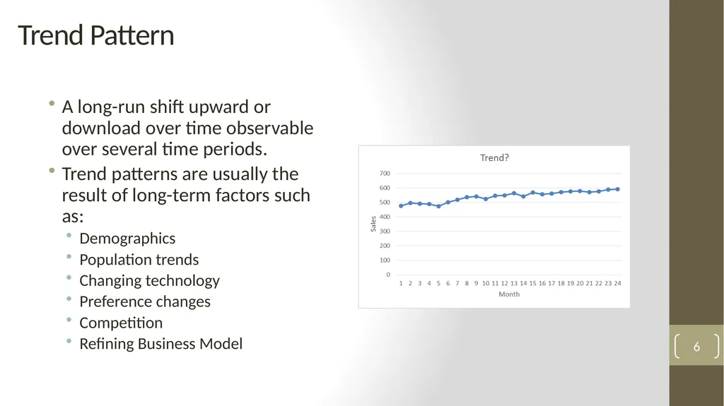
Trend Pattern A long-run shift upward or download over time observable over several time periods.
Trend patterns are usually the result of long-term factors such as:
Demographics
Population trends
Changing technology
Preference changes
Competition
Refining Business Model 6<br>
Trend patterns are usually the result of long-term factors such as:
Demographics
Population trends
Changing technology
Preference changes
Competition
Refining Business Model 6<br>
07
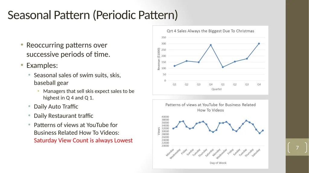
Seasonal Pattern (Periodic Pattern) Reoccurring patterns over successive periods of time.
Examples:
Seasonal sales of swim suits, skis, baseball gear
Managers that sell skis expect sales to be highest in Q 4 and Q 1.
Daily Auto Traffic
Daily Restaurant traffic
Patterns of views at YouTube for Business Related How To Videos: Saturday View Count is always Lowest 7<br>
Examples:
Seasonal sales of swim suits, skis, baseball gear
Managers that sell skis expect sales to be highest in Q 4 and Q 1.
Daily Auto Traffic
Daily Restaurant traffic
Patterns of views at YouTube for Business Related How To Videos: Saturday View Count is always Lowest 7<br>
08
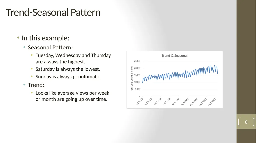
Trend-Seasonal Pattern In this example:
Seasonal Pattern:
Tuesday, Wednesday and Thursday are always the highest.
Saturday is always the lowest.
Sunday is always penultimate.
Trend:
Looks like average views per week or month are going up over time. 8<br>
Seasonal Pattern:
Tuesday, Wednesday and Thursday are always the highest.
Saturday is always the lowest.
Sunday is always penultimate.
Trend:
Looks like average views per week or month are going up over time. 8<br>
09
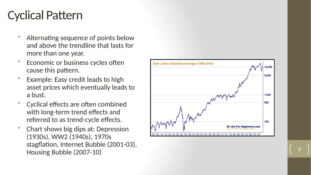
Cyclical Pattern Alternating sequence of points below and above the trendline that lasts for more than one year.
Economic or business cycles often cause this pattern.
Example: Easy credit leads to high asset prices which eventually leads to a bust.
Cyclical effects are often combined with long-term trend effects and referred to as trend-cycle effects.
Chart shows big dips at: Depression (1930s), WW2 (1940s), 1970s stagflation, Internet Bubble (2001-03), Housing Bubble (2007-10) 9<br>
Economic or business cycles often cause this pattern.
Example: Easy credit leads to high asset prices which eventually leads to a bust.
Cyclical effects are often combined with long-term trend effects and referred to as trend-cycle effects.
Chart shows big dips at: Depression (1930s), WW2 (1940s), 1970s stagflation, Internet Bubble (2001-03), Housing Bubble (2007-10) 9<br>
10
Basic Forecasting Methods For Constant or Horizontal or Stationary Pattern:
Most Recent (Naïve Forecast Method)
Average of Past Values
Moving Averages
Exponential Smoothing
Trends:
Regression Analysis 10<br>
Most Recent (Naïve Forecast Method)
Average of Past Values
Moving Averages
Exponential Smoothing
Trends:
Regression Analysis 10<br>
11
Measure of Forecast Accuracy Forecast Error
Mean Forecast Error = MFE
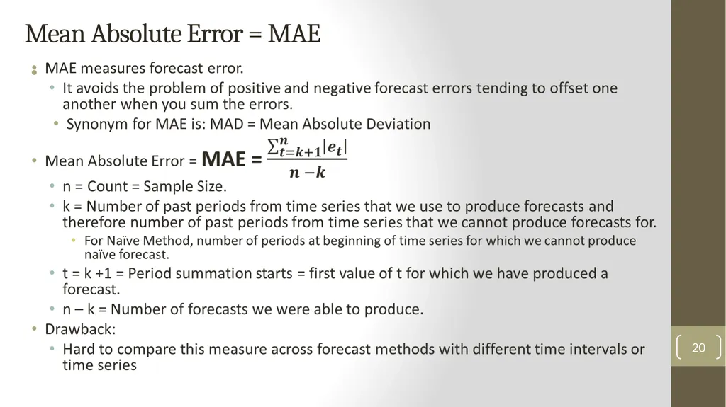
Mean Absolute Error = MAE
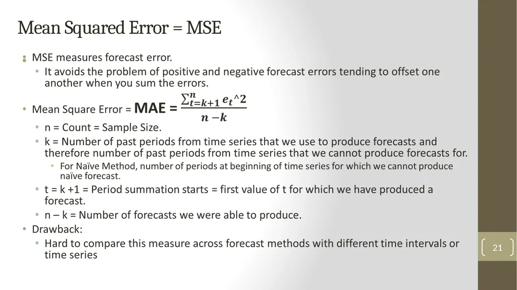
Mean Squared Error = MSE
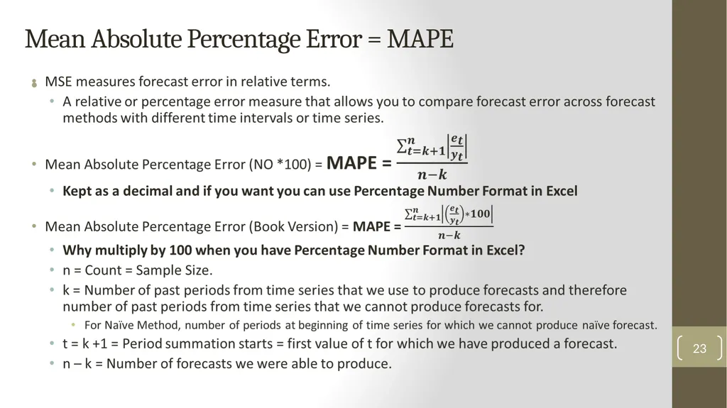
Mean Absolute Percentage Error = MAPE 11<br>
Mean Forecast Error = MFE
Mean Absolute Error = MAE
Mean Squared Error = MSE
Mean Absolute Percentage Error = MAPE 11<br>
12
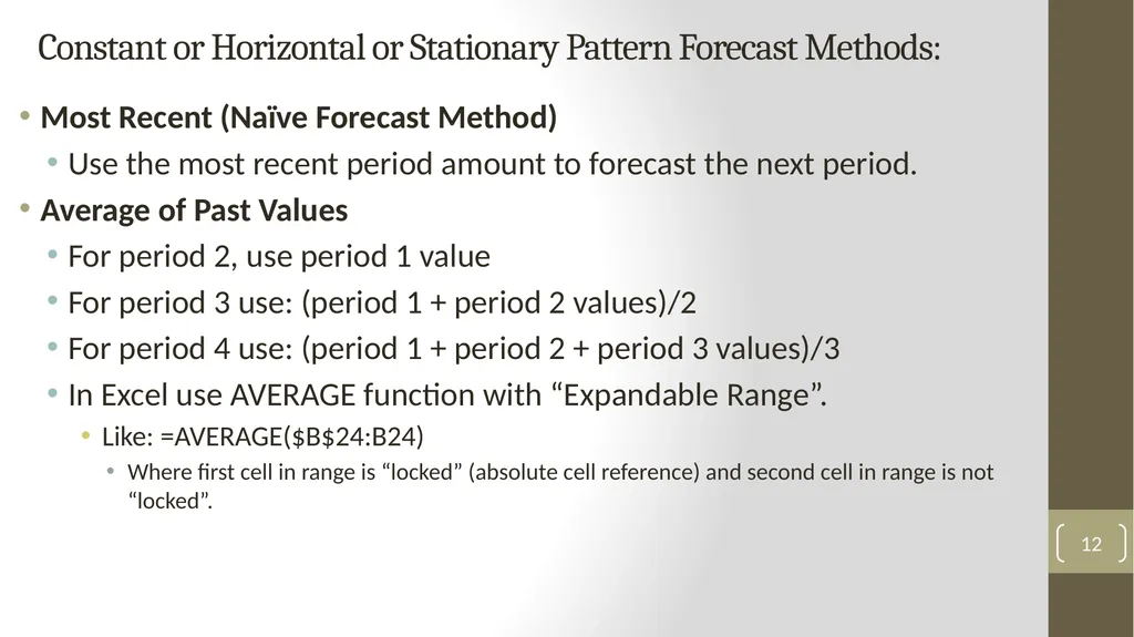
Constant or Horizontal or Stationary Pattern Forecast Methods: Most Recent (Naïve Forecast Method)
Use the most recent period amount to forecast the next period.
Average of Past Values
For period 2, use period 1 value
For period 3 use: (period 1 + period 2 values)/2
For period 4 use: (period 1 + period 2 + period 3 values)/3
In Excel use AVERAGE function with “Expandable Range”.
Like: =AVERAGE($B$24:B24)
Where first cell in range is “locked” (absolute cell reference) and second cell in range is not “locked”. 12<br>
Use the most recent period amount to forecast the next period.
Average of Past Values
For period 2, use period 1 value
For period 3 use: (period 1 + period 2 values)/2
For period 4 use: (period 1 + period 2 + period 3 values)/3
In Excel use AVERAGE function with “Expandable Range”.
Like: =AVERAGE($B$24:B24)
Where first cell in range is “locked” (absolute cell reference) and second cell in range is not “locked”. 12<br>
13
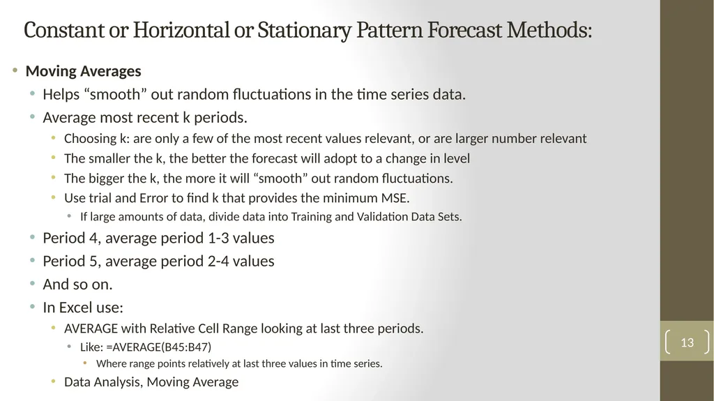
Constant or Horizontal or Stationary Pattern Forecast Methods: Moving Averages
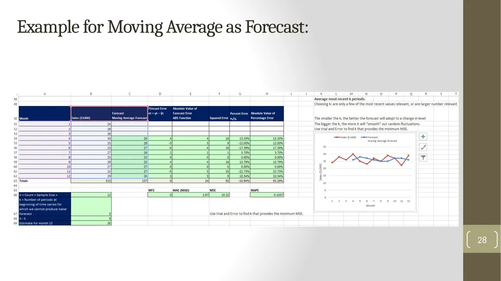
Helps “smooth” out random fluctuations in the time series data.
Average most recent k periods.
Choosing k: are only a few of the most recent values relevant, or are larger number relevant
The smaller the k, the better the forecast will adopt to a change in level
The bigger the k, the more it will “smooth” out random fluctuations.
Use trial and Error to find k that provides the minimum MSE.
If large amounts of data, divide data into Training and Validation Data Sets.
Period 4, average period 1-3 values
Period 5, average period 2-4 values
And so on.
In Excel use:
AVERAGE with Relative Cell Range looking at last three periods.
Like: =AVERAGE(B45:B47)
Where range points relatively at last three values in time series.
Data Analysis, Moving Average 13<br>
Helps “smooth” out random fluctuations in the time series data.
Average most recent k periods.
Choosing k: are only a few of the most recent values relevant, or are larger number relevant
The smaller the k, the better the forecast will adopt to a change in level
The bigger the k, the more it will “smooth” out random fluctuations.
Use trial and Error to find k that provides the minimum MSE.
If large amounts of data, divide data into Training and Validation Data Sets.
Period 4, average period 1-3 values
Period 5, average period 2-4 values
And so on.
In Excel use:
AVERAGE with Relative Cell Range looking at last three periods.
Like: =AVERAGE(B45:B47)
Where range points relatively at last three values in time series.
Data Analysis, Moving Average 13<br>
14
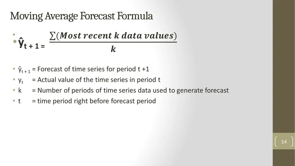
Moving Average Forecast Formula 14<br>
15
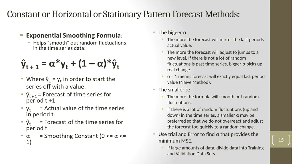
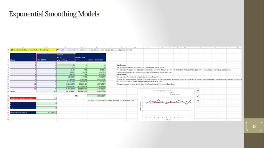
Constant or Horizontal or Stationary Pattern Forecast Methods: The bigger α:
The more the forecast will mirror the last periods actual value.
The more the forecast will adjust to jumps to a new level. If there is not a lot of random fluctuations is past time series, bigger α picks up real change.
α = 1 means forecast will exactly equal last period value (Naïve Method).
The smaller α:
The more the formula will smooth out random fluctuations.
If there is a lot of random fluctuations (up and down) in the time series, a smaller α may be preferred so that we do not overreact and adjust the forecast too quickly to a random change.
Use trial and Error to find α that provides the minimum MSE.
If large amounts of data, divide data into Training and Validation Data Sets. 15<br>
The more the forecast will mirror the last periods actual value.
The more the forecast will adjust to jumps to a new level. If there is not a lot of random fluctuations is past time series, bigger α picks up real change.
α = 1 means forecast will exactly equal last period value (Naïve Method).
The smaller α:
The more the formula will smooth out random fluctuations.
If there is a lot of random fluctuations (up and down) in the time series, a smaller α may be preferred so that we do not overreact and adjust the forecast too quickly to a random change.
Use trial and Error to find α that provides the minimum MSE.
If large amounts of data, divide data into Training and Validation Data Sets. 15<br>
16
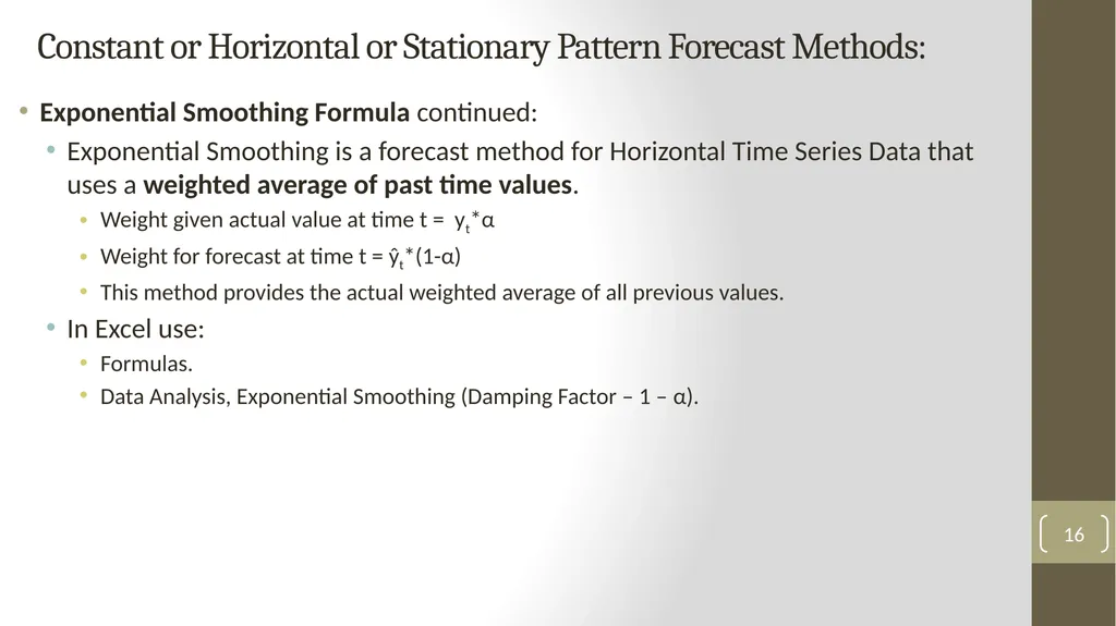
Constant or Horizontal or Stationary Pattern Forecast Methods: Exponential Smoothing Formula continued:
Exponential Smoothing is a forecast method for Horizontal Time Series Data that uses a weighted average of past time values.
Weight given actual value at time t = yt*α
Weight for forecast at time t = ŷt*(1-α)
This method provides the actual weighted average of all previous values.
In Excel use:
Formulas.
Data Analysis, Exponential Smoothing (Damping Factor – 1 – α). 16<br>
Exponential Smoothing is a forecast method for Horizontal Time Series Data that uses a weighted average of past time values.
Weight given actual value at time t = yt*α
Weight for forecast at time t = ŷt*(1-α)
This method provides the actual weighted average of all previous values.
In Excel use:
Formulas.
Data Analysis, Exponential Smoothing (Damping Factor – 1 – α). 16<br>
17
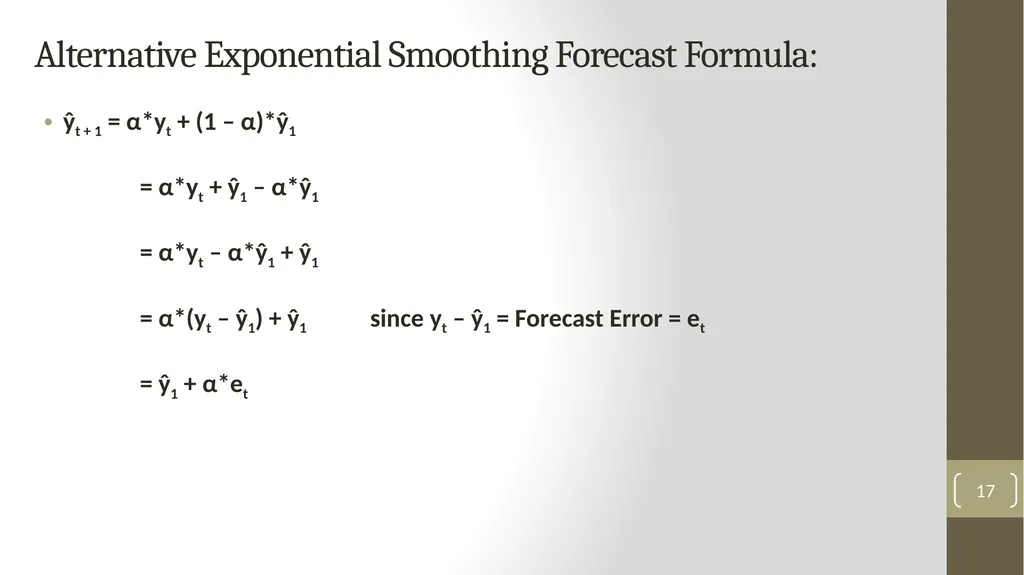
Alternative Exponential Smoothing Forecast Formula: ŷt + 1 = α*yt + (1 – α)*ŷ1
= α*yt + ŷ1 – α*ŷ1
= α*yt – α*ŷ1 + ŷ1
= α*(yt – ŷ1) + ŷ1 since yt – ŷ1 = Forecast Error = et
= ŷ1 + α*et 17<br>
18
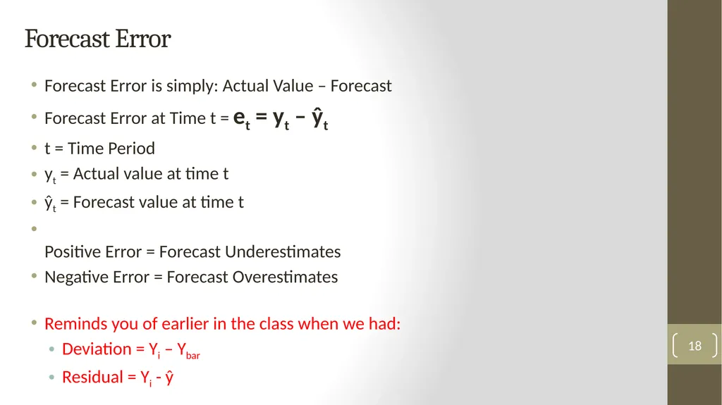
Forecast Error Forecast Error is simply: Actual Value – Forecast
Forecast Error at Time t = et = yt – ŷt
t = Time Period
yt = Actual value at time t
ŷt = Forecast value at time t
Positive Error = Forecast Underestimates
Negative Error = Forecast Overestimates
Reminds you of earlier in the class when we had:
Deviation = Yi – Ybar
Residual = Yi - ŷ 18<br>
Forecast Error at Time t = et = yt – ŷt
t = Time Period
yt = Actual value at time t
ŷt = Forecast value at time t
Positive Error = Forecast Underestimates
Negative Error = Forecast Overestimates
Reminds you of earlier in the class when we had:
Deviation = Yi – Ybar
Residual = Yi - ŷ 18<br>
19
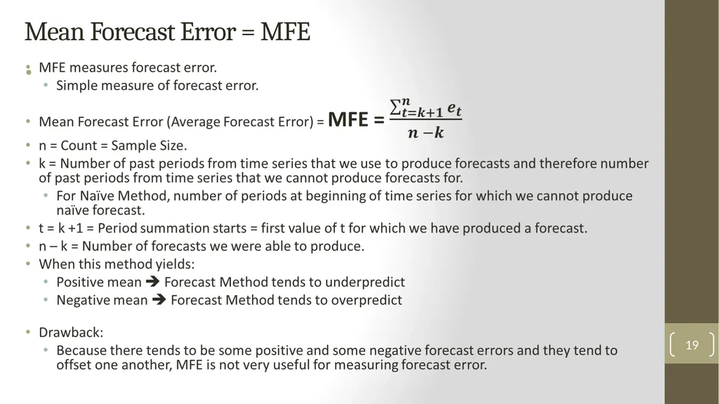
Mean Forecast Error = MFE 19<br>
20
Mean Absolute Error = MAE 20<br>
21
Mean Squared Error = MSE 21<br>
22
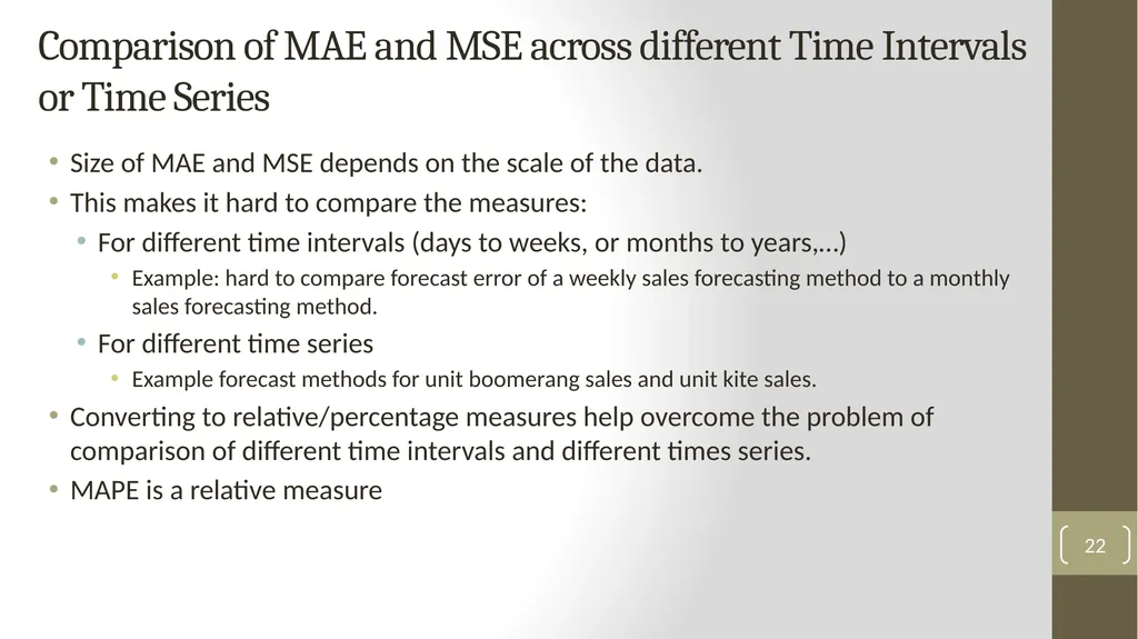
Comparison of MAE and MSE across different Time Intervals or Time Series Size of MAE and MSE depends on the scale of the data.
This makes it hard to compare the measures:
For different time intervals (days to weeks, or months to years,…)
Example: hard to compare forecast error of a weekly sales forecasting method to a monthly sales forecasting method.
For different time series
Example forecast methods for unit boomerang sales and unit kite sales.
Converting to relative/percentage measures help overcome the problem of comparison of different time intervals and different times series.
MAPE is a relative measure 22<br>
This makes it hard to compare the measures:
For different time intervals (days to weeks, or months to years,…)
Example: hard to compare forecast error of a weekly sales forecasting method to a monthly sales forecasting method.
For different time series
Example forecast methods for unit boomerang sales and unit kite sales.
Converting to relative/percentage measures help overcome the problem of comparison of different time intervals and different times series.
MAPE is a relative measure 22<br>
23
Mean Absolute Percentage Error = MAPE 23<br>
24
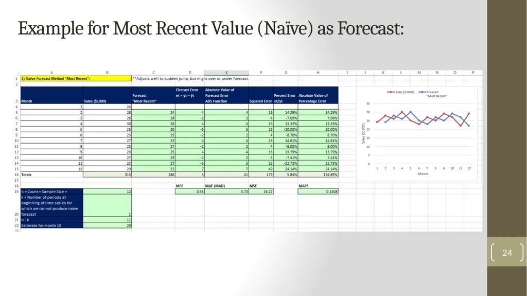
Example for Most Recent Value (Naïve) as Forecast: 24<br>
25
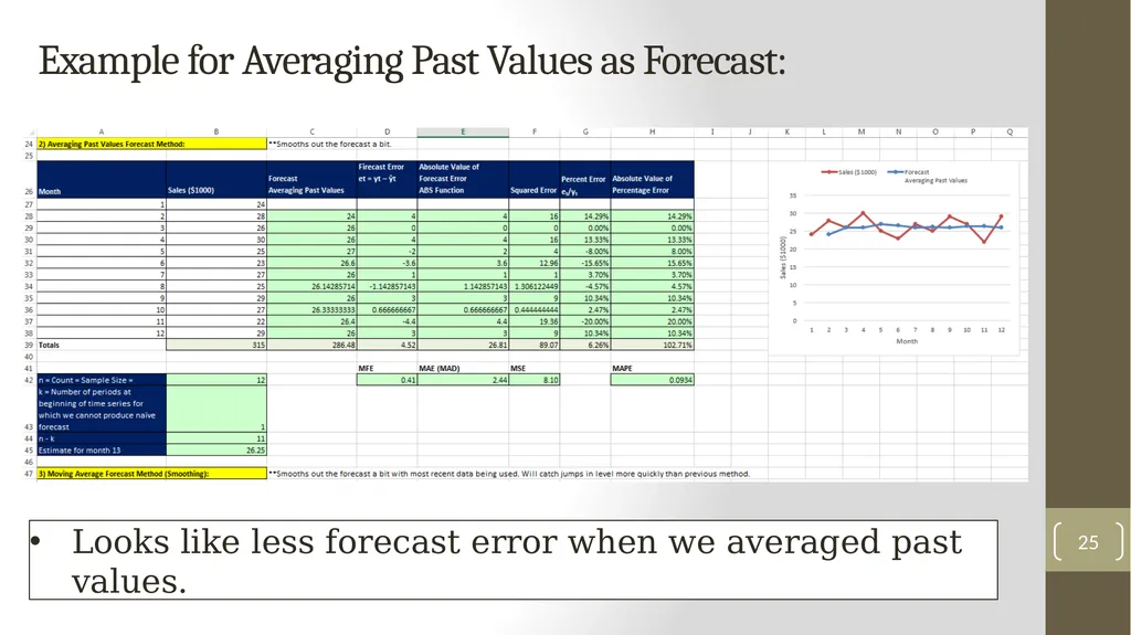
25 Example for Averaging Past Values as Forecast: Looks like less forecast error when we averaged past values.<br>
26
Naïve Method Vs. Averaging Past Values If values are stationary, the average method tends to be more accurate.
If there is a big jump up or down (like chart on slide 8), naïve method will reflect the change more quickly than the average method. 26<br>
If there is a big jump up or down (like chart on slide 8), naïve method will reflect the change more quickly than the average method. 26<br>
27
Moving Average & Exponential Smoothing Moving Average & Exponential Smoothing appropriate for Horizontal Pattern
Can adapt to sudden changes in Level
However, without modification they are not appropriate for:
Trend
Cyclical
Seasonal
Objective of methods:
Smooth out random fluctuations
Moving Average & Exponential Smoothing are good for short term forecast, like next period. 27<br>
Can adapt to sudden changes in Level
However, without modification they are not appropriate for:
Trend
Cyclical
Seasonal
Objective of methods:
Smooth out random fluctuations
Moving Average & Exponential Smoothing are good for short term forecast, like next period. 27<br>
28
Example for Moving Average as Forecast: 28<br>
29
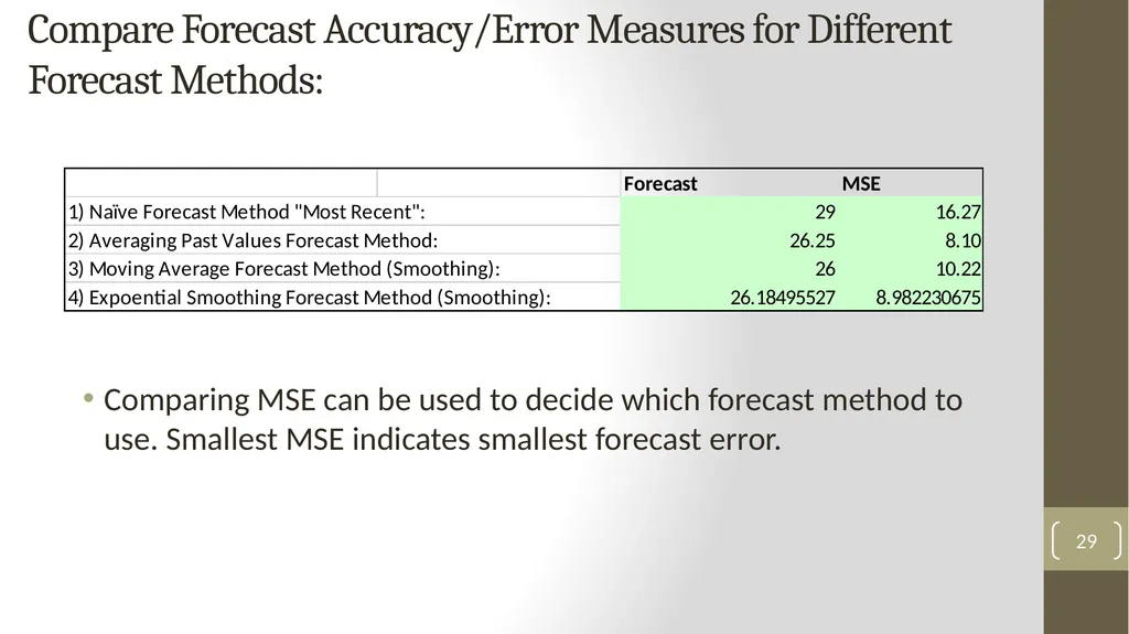
Compare Forecast Accuracy/Error Measures for Different Forecast Methods: Comparing MSE can be used to decide which forecast method to use. Smallest MSE indicates smallest forecast error. 29<br>
30
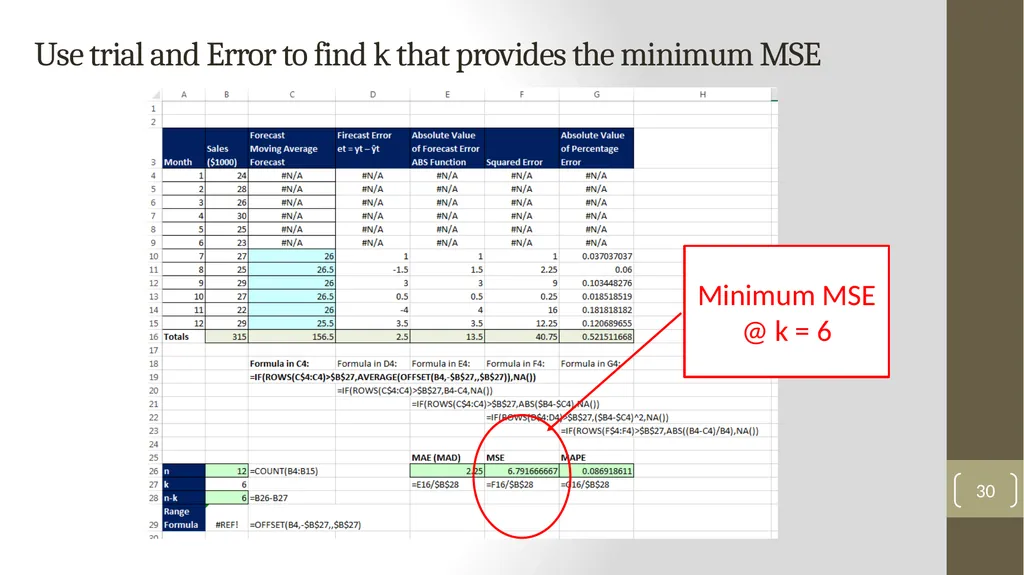
Use trial and Error to find k that provides the minimum MSE 30 Minimum MSE @ k = 6<br>
31
Forecast Error for Future Forecast? MAE, MSE and MAPE only can measure how well forecast method works on forecasting historical values of the time series…
No way to measure forecast error of future estimates… It is the unknown future…
However, our goal is been to check if the forecasting method works on historical values.
If our assumption that the past is a good estimate of the future, then this process helps us assess the accuracy of the method. 31<br>
No way to measure forecast error of future estimates… It is the unknown future…
However, our goal is been to check if the forecasting method works on historical values.
If our assumption that the past is a good estimate of the future, then this process helps us assess the accuracy of the method. 31<br>
32
Historical Data and Good Business Judgment Using Historical Data to estimate what might happen in the future is important.
Good knowledge of business and economic environment are also important. 32<br>
Good knowledge of business and economic environment are also important. 32<br>
33
Exponential Smoothing Models 33<br>
34
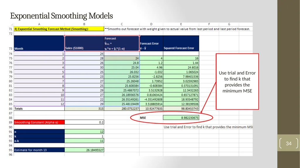
Exponential Smoothing Models 34 Use trial and Error to find k that provides the minimum MSE<br>
35
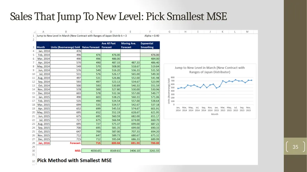
Sales That Jump To New Level: Pick Smallest MSE 35<br>
36
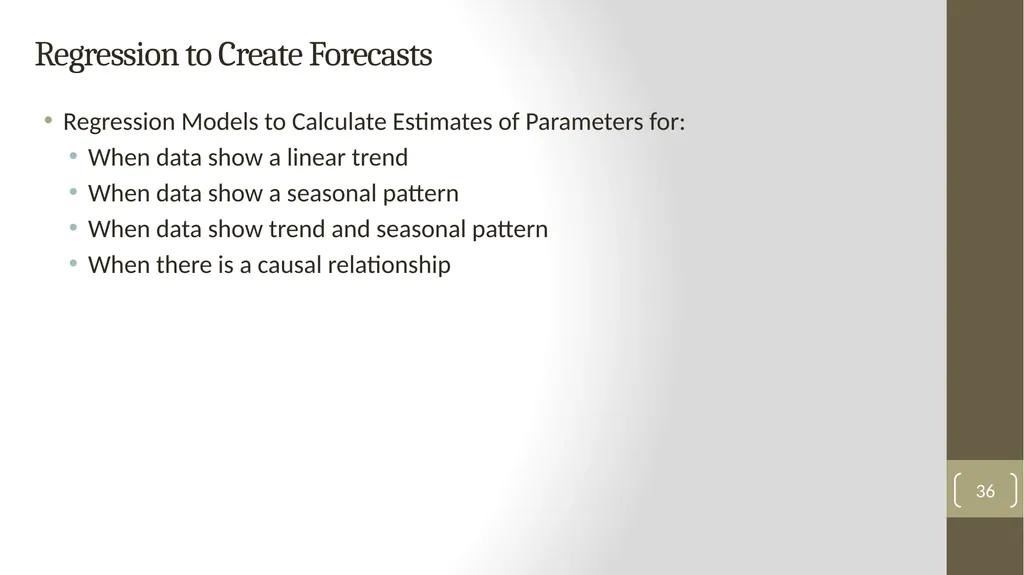
Regression to Create Forecasts Regression Models to Calculate Estimates of Parameters for:
When data show a linear trend
When data show a seasonal pattern
When data show trend and seasonal pattern
When there is a causal relationship 36<br>
When data show a linear trend
When data show a seasonal pattern
When data show trend and seasonal pattern
When there is a causal relationship 36<br>
37
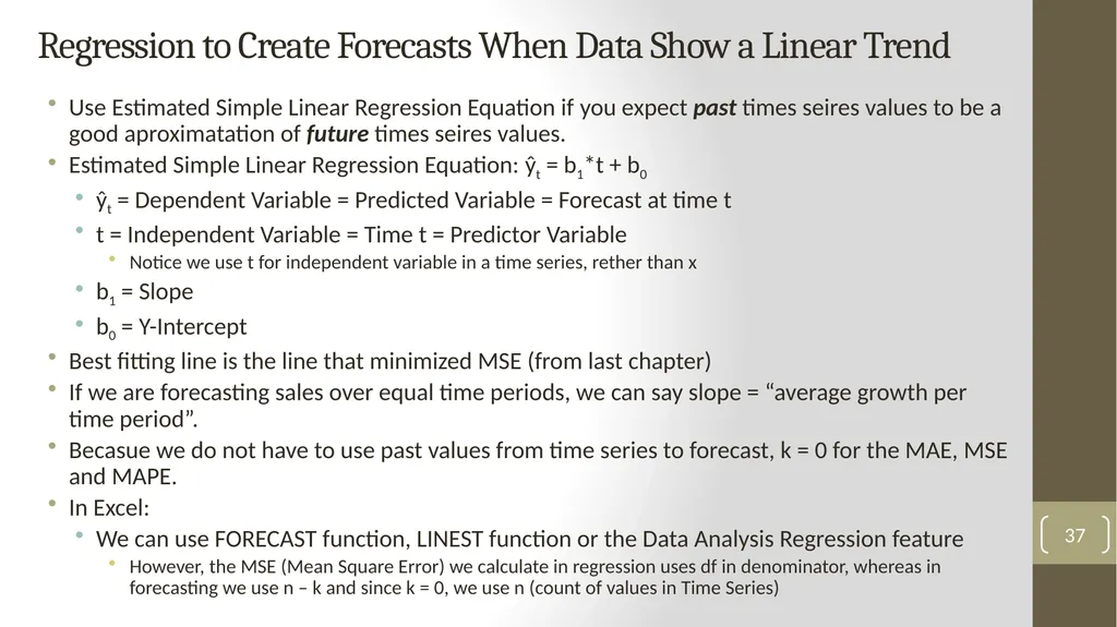
Regression to Create Forecasts When Data Show a Linear Trend Use Estimated Simple Linear Regression Equation if you expect past times seires values to be a good aproximatation of future times seires values.
Estimated Simple Linear Regression Equation: ŷt = b1*t + b0
ŷt = Dependent Variable = Predicted Variable = Forecast at time t
t = Independent Variable = Time t = Predictor Variable
Notice we use t for independent variable in a time series, rether than x
b1 = Slope
b0 = Y-Intercept
Best fitting line is the line that minimized MSE (from last chapter)
If we are forecasting sales over equal time periods, we can say slope = “average growth per time period”.
Becasue we do not have to use past values from time series to forecast, k = 0 for the MAE, MSE and MAPE.
In Excel:
We can use FORECAST function, LINEST function or the Data Analysis Regression feature
However, the MSE (Mean Square Error) we calculate in regression uses df in denominator, whereas in forecasting we use n – k and since k = 0, we use n (count of values in Time Series) 37<br>
Estimated Simple Linear Regression Equation: ŷt = b1*t + b0
ŷt = Dependent Variable = Predicted Variable = Forecast at time t
t = Independent Variable = Time t = Predictor Variable
Notice we use t for independent variable in a time series, rether than x
b1 = Slope
b0 = Y-Intercept
Best fitting line is the line that minimized MSE (from last chapter)
If we are forecasting sales over equal time periods, we can say slope = “average growth per time period”.
Becasue we do not have to use past values from time series to forecast, k = 0 for the MAE, MSE and MAPE.
In Excel:
We can use FORECAST function, LINEST function or the Data Analysis Regression feature
However, the MSE (Mean Square Error) we calculate in regression uses df in denominator, whereas in forecasting we use n – k and since k = 0, we use n (count of values in Time Series) 37<br>
38
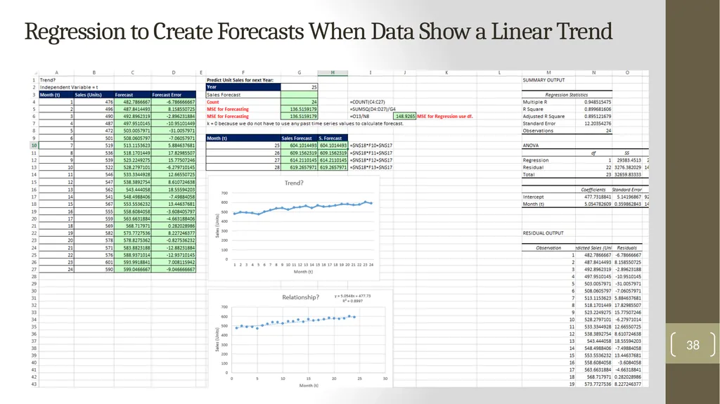
Regression to Create Forecasts When Data Show a Linear Trend 38<br>
39
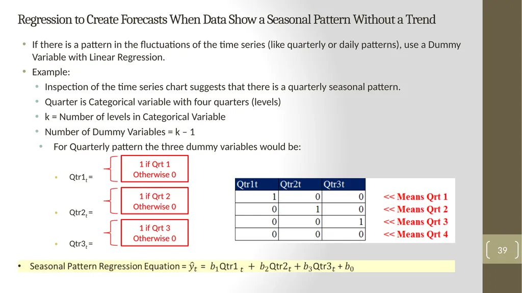
Regression to Create Forecasts When Data Show a Seasonal Pattern Without a Trend If there is a pattern in the fluctuations of the time series (like quarterly or daily patterns), use a Dummy Variable with Linear Regression.
Example:
Inspection of the time series chart suggests that there is a quarterly seasonal pattern.
Quarter is Categorical variable with four quarters (levels)
k = Number of levels in Categorical Variable
Number of Dummy Variables = k – 1
For Quarterly pattern the three dummy variables would be:
Qtr1t =
Qtr2t =
Qtr3t = 39 1 if Qrt 1
Otherwise 0 1 if Qrt 2
Otherwise 0 1 if Qrt 3
Otherwise 0<br>
Example:
Inspection of the time series chart suggests that there is a quarterly seasonal pattern.
Quarter is Categorical variable with four quarters (levels)
k = Number of levels in Categorical Variable
Number of Dummy Variables = k – 1
For Quarterly pattern the three dummy variables would be:
Qtr1t =
Qtr2t =
Qtr3t = 39 1 if Qrt 1
Otherwise 0 1 if Qrt 2
Otherwise 0 1 if Qrt 3
Otherwise 0<br>
40
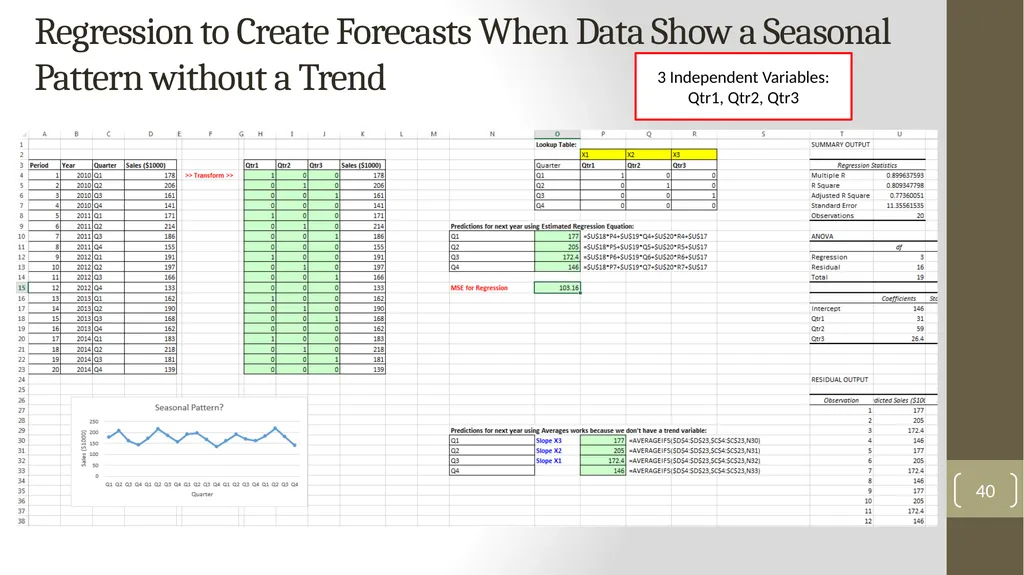
Regression to Create Forecasts When Data Show a Seasonal Pattern without a Trend 40 3 Independent Variables: Qtr1, Qtr2, Qtr3<br>
41
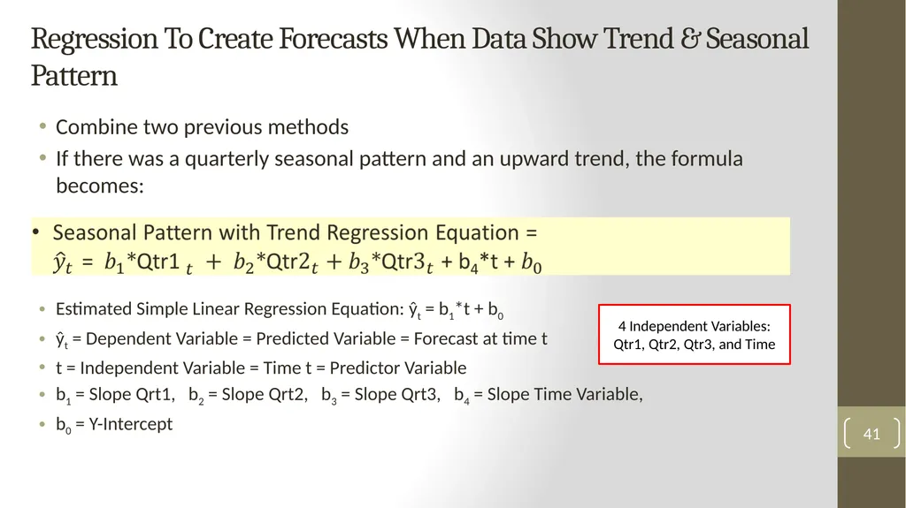
Regression To Create Forecasts When Data Show Trend & Seasonal Pattern Combine two previous methods
If there was a quarterly seasonal pattern and an upward trend, the formula becomes:
Estimated Simple Linear Regression Equation: ŷt = b1*t + b0
ŷt = Dependent Variable = Predicted Variable = Forecast at time t
t = Independent Variable = Time t = Predictor Variable
b1 = Slope Qrt1, b2 = Slope Qrt2, b3 = Slope Qrt3, b4 = Slope Time Variable,
b0 = Y-Intercept 41 4 Independent Variables: Qtr1, Qtr2, Qtr3, and Time<br>
If there was a quarterly seasonal pattern and an upward trend, the formula becomes:
Estimated Simple Linear Regression Equation: ŷt = b1*t + b0
ŷt = Dependent Variable = Predicted Variable = Forecast at time t
t = Independent Variable = Time t = Predictor Variable
b1 = Slope Qrt1, b2 = Slope Qrt2, b3 = Slope Qrt3, b4 = Slope Time Variable,
b0 = Y-Intercept 41 4 Independent Variables: Qtr1, Qtr2, Qtr3, and Time<br>
42
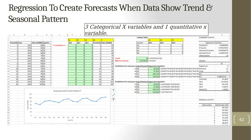
Regression To Create Forecasts When Data Show Trend & Seasonal Pattern 42 3 Categorical X variables and 1 quantitative x variable.<br>
43
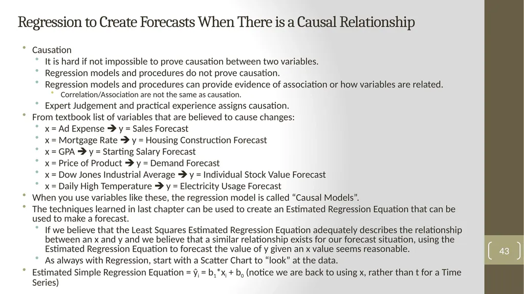
Regression to Create Forecasts When There is a Causal Relationship Causation
It is hard if not impossible to prove causation between two variables.
Regression models and procedures do not prove causation.
Regression models and procedures can provide evidence of association or how variables are related.
Correlation/Association are not the same as causation.
Expert Judgement and practical experience assigns causation.
From textbook list of variables that are believed to cause changes:
x = Ad Expense y = Sales Forecast
x = Mortgage Rate y = Housing Construction Forecast
x = GPA y = Starting Salary Forecast
x = Price of Product y = Demand Forecast
x = Dow Jones Industrial Average y = Individual Stock Value Forecast
x = Daily High Temperature y = Electricity Usage Forecast
When you use variables like these, the regression model is called “Causal Models”.
The techniques learned in last chapter can be used to create an Estimated Regression Equation that can be used to make a forecast.
If we believe that the Least Squares Estimated Regression Equation adequately describes the relationship between an x and y and we believe that a similar relationship exists for our forecast situation, using the Estimated Regression Equation to forecast the value of y given an x value seems reasonable.
As always with Regression, start with a Scatter Chart to “look” at the data.
Estimated Simple Regression Equation = ŷi = b1*xi + b0 (notice we are back to using x, rather than t for a Time Series) 43<br>
It is hard if not impossible to prove causation between two variables.
Regression models and procedures do not prove causation.
Regression models and procedures can provide evidence of association or how variables are related.
Correlation/Association are not the same as causation.
Expert Judgement and practical experience assigns causation.
From textbook list of variables that are believed to cause changes:
x = Ad Expense y = Sales Forecast
x = Mortgage Rate y = Housing Construction Forecast
x = GPA y = Starting Salary Forecast
x = Price of Product y = Demand Forecast
x = Dow Jones Industrial Average y = Individual Stock Value Forecast
x = Daily High Temperature y = Electricity Usage Forecast
When you use variables like these, the regression model is called “Causal Models”.
The techniques learned in last chapter can be used to create an Estimated Regression Equation that can be used to make a forecast.
If we believe that the Least Squares Estimated Regression Equation adequately describes the relationship between an x and y and we believe that a similar relationship exists for our forecast situation, using the Estimated Regression Equation to forecast the value of y given an x value seems reasonable.
As always with Regression, start with a Scatter Chart to “look” at the data.
Estimated Simple Regression Equation = ŷi = b1*xi + b0 (notice we are back to using x, rather than t for a Time Series) 43<br>
44
Combining Causal Variables with Trends and Seasonal Effects. Example: combine regression techniques for all three:
Causal Variable like Ad Expense to predict Sales
Trend from a past data time series
Seasonal Effects 44<br>
Causal Variable like Ad Expense to predict Sales
Trend from a past data time series
Seasonal Effects 44<br>
45
Considerations When Using Regression for Forecasting Page 236 in textbook:
Whether a regression approach provides a good forecast depends largely on
How well we are able to identify and obtain data for independent variables that are closely related to the time series.
Part of the regression analysis procedure should focus on the selection of the set of independent variables that provides the best forecasting model. 45<br>
Whether a regression approach provides a good forecast depends largely on
How well we are able to identify and obtain data for independent variables that are closely related to the time series.
Part of the regression analysis procedure should focus on the selection of the set of independent variables that provides the best forecasting model. 45<br>
46
Determining Best Forecast Model Lots of trial and error.
Large Time series, break set into two parts:
Training Set: use earlier year to try different methods and find a good model
Validation Set: Use model from Training Set to verify on this second set.
Be wary of changes through long periods of time.
Try to pick model that minimizes errors, such as MSE. 46<br>
Large Time series, break set into two parts:
Training Set: use earlier year to try different methods and find a good model
Validation Set: Use model from Training Set to verify on this second set.
Be wary of changes through long periods of time.
Try to pick model that minimizes errors, such as MSE. 46<br>
47
Other Methods Not Covered In This Class Moving Averages & Exponential Smoothing Only the Start
Moving Averages & Exponential Smoothing are the foundation for more advanced formulas such as:
Weighted Moving Averages
Double Moving Averages
Brown's Method for Double Exponential Smoothing
Triple Exponential Smoothing
More…
Regression with Nonlinear Trends
Autoregressive Models
Regression with independent variables from k previous period time series values (each a separate independent variable). Formula is used to predict future time series values.
Holt-Winters Seasonal Smoothing
Holt-Winters Multiplicative Method 47<br>
Moving Averages & Exponential Smoothing are the foundation for more advanced formulas such as:
Weighted Moving Averages
Double Moving Averages
Brown's Method for Double Exponential Smoothing
Triple Exponential Smoothing
More…
Regression with Nonlinear Trends
Autoregressive Models
Regression with independent variables from k previous period time series values (each a separate independent variable). Formula is used to predict future time series values.
Holt-Winters Seasonal Smoothing
Holt-Winters Multiplicative Method 47<br>
48
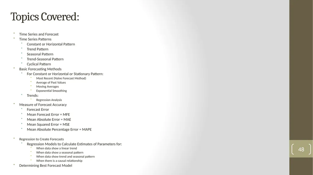
Topics Covered: Time Series and Forecast
Time Series Patterns
Constant or Horizontal Pattern
Trend Pattern
Seasonal Pattern
Trend-Seasonal Pattern
Cyclical Pattern
Basic Forecasting Methods
For Constant or Horizontal or Stationary Pattern:
Most Recent (Naïve Forecast Method)
Average of Past Values
Moving Averages
Exponential Smoothing
Trends:
Regression Analysis
Measure of Forecast Accuracy
Forecast Error
Mean Forecast Error = MFE
Mean Absolute Error = MAE
Mean Squared Error = MSE
Mean Absolute Percentage Error = MAPE
Regression to Create Forecasts
Regression Models to Calculate Estimates of Parameters for:
When data show a linear trend
When data show a seasonal pattern
When data show trend and seasonal pattern
When there is a causal relationship
Determining Best Forecast Model 48<br>
Time Series Patterns
Constant or Horizontal Pattern
Trend Pattern
Seasonal Pattern
Trend-Seasonal Pattern
Cyclical Pattern
Basic Forecasting Methods
For Constant or Horizontal or Stationary Pattern:
Most Recent (Naïve Forecast Method)
Average of Past Values
Moving Averages
Exponential Smoothing
Trends:
Regression Analysis
Measure of Forecast Accuracy
Forecast Error
Mean Forecast Error = MFE
Mean Absolute Error = MAE
Mean Squared Error = MSE
Mean Absolute Percentage Error = MAPE
Regression to Create Forecasts
Regression Models to Calculate Estimates of Parameters for:
When data show a linear trend
When data show a seasonal pattern
When data show trend and seasonal pattern
When there is a causal relationship
Determining Best Forecast Model 48<br>