04
HW 2 Because the due date for HW 2 has gotten pushed back a week (now due Monday, 2/10), the next hw was dropped and instead I’ve added some problems to HW corresponding to today’s class
If you already downloaded it, make sure to look at the updated version<br>
06
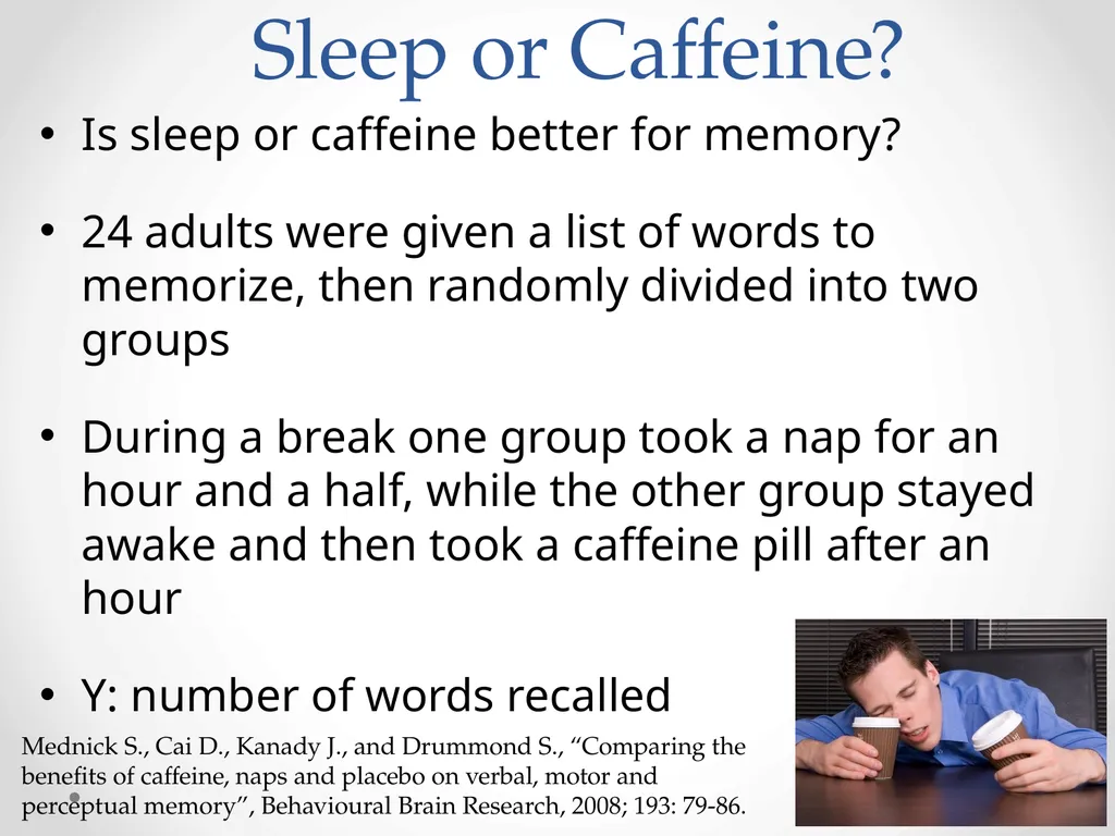
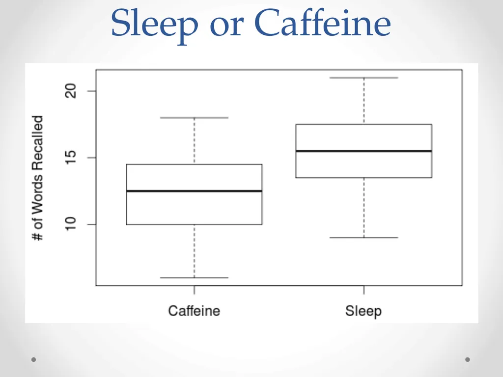
Sleep or Caffeine? Is sleep or caffeine better for memory?
24 adults were given a list of words to memorize, then randomly divided into two groups
During a break one group took a nap for an hour and a half, while the other group stayed awake and then took a caffeine pill after an hour
Y: number of words recalled Mednick S., Cai D., Kanady J., and Drummond S., “Comparing the benefits of caffeine, naps and placebo on verbal, motor and perceptual memory”, Behavioural Brain Research, 2008; 193: 79-86.<br>
08
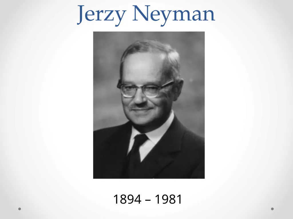
Jerzy Neyman 1894 – 1981<br>
09
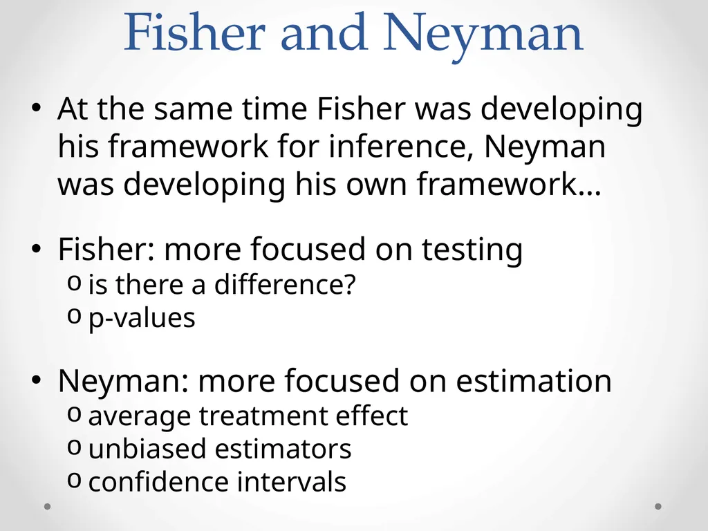
Fisher and Neyman At the same time Fisher was developing his framework for inference, Neyman was developing his own framework…
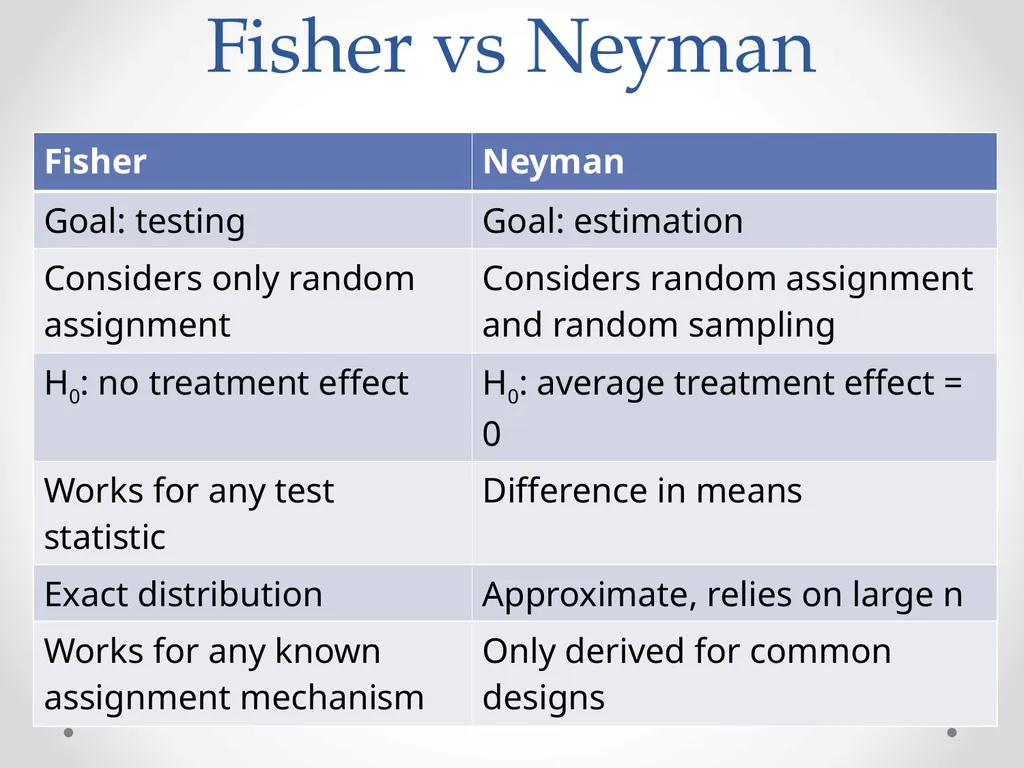
Fisher: more focused on testing
is there a difference?
p-values
Neyman: more focused on estimation
average treatment effect
unbiased estimators
confidence intervals<br>
10
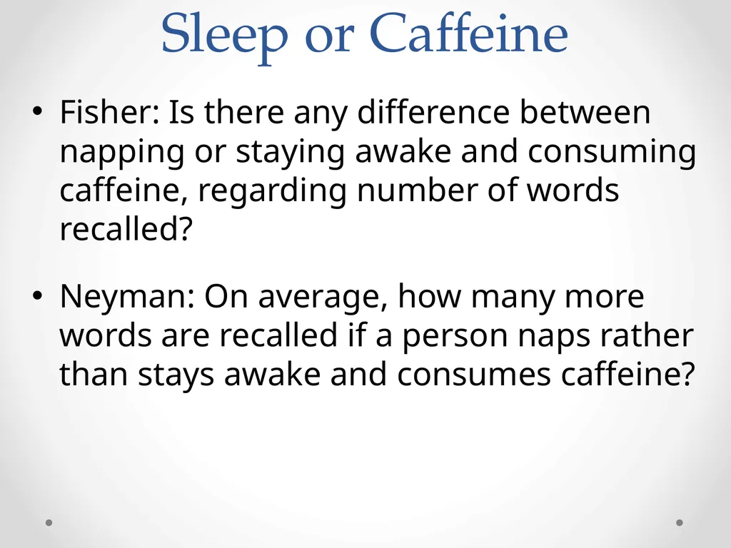
Sleep or Caffeine Fisher: Is there any difference between napping or staying awake and consuming caffeine, regarding number of words recalled?
Neyman: On average, how many more words are recalled if a person naps rather than stays awake and consumes caffeine?<br>
11
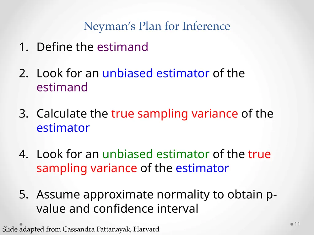
Neyman’s Plan for Inference Define the estimand
Look for an unbiased estimator of the estimand
Calculate the true sampling variance of the estimator
Look for an unbiased estimator of the true sampling variance of the estimator
Assume approximate normality to obtain p-value and confidence interval 11 Slide adapted from Cassandra Pattanayak, Harvard<br>
12
Finite Sample vs Super Population Finite sample inference:
Only concerned with units in the sample
Only source of randomness is random assignment to treatment groups
(Fisher exact p-values)
Super population inference:
Extend inferences to greater population
Two sources of randomness: random sampling, random assignment
“repeated sampling”
We’ll first explore finite sample inference…<br>
13
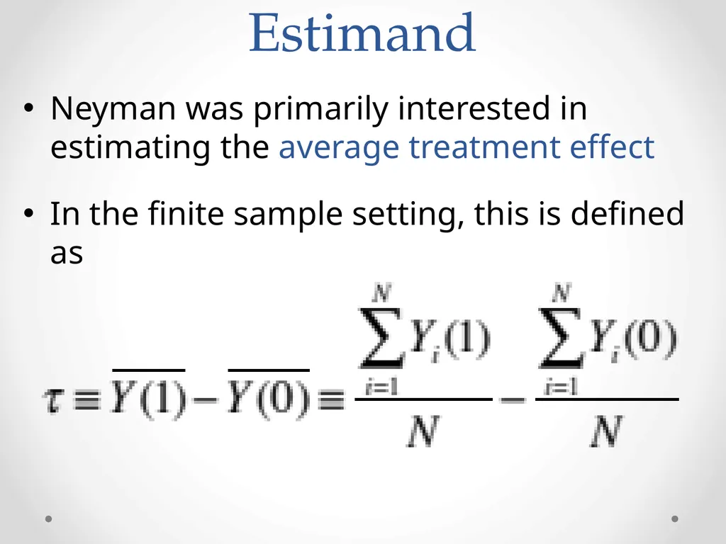
Estimand Neyman was primarily interested in estimating the average treatment effect
In the finite sample setting, this is defined as<br>
14
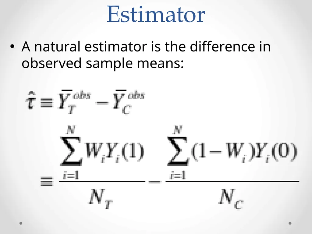
Estimator A natural estimator is the difference in observed sample means:<br>
15
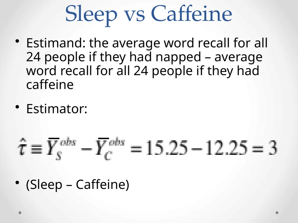
Sleep vs Caffeine Estimand: the average word recall for all 24 people if they had napped – average word recall for all 24 people if they had caffeine
Estimator:
(Sleep – Caffeine)<br>
16
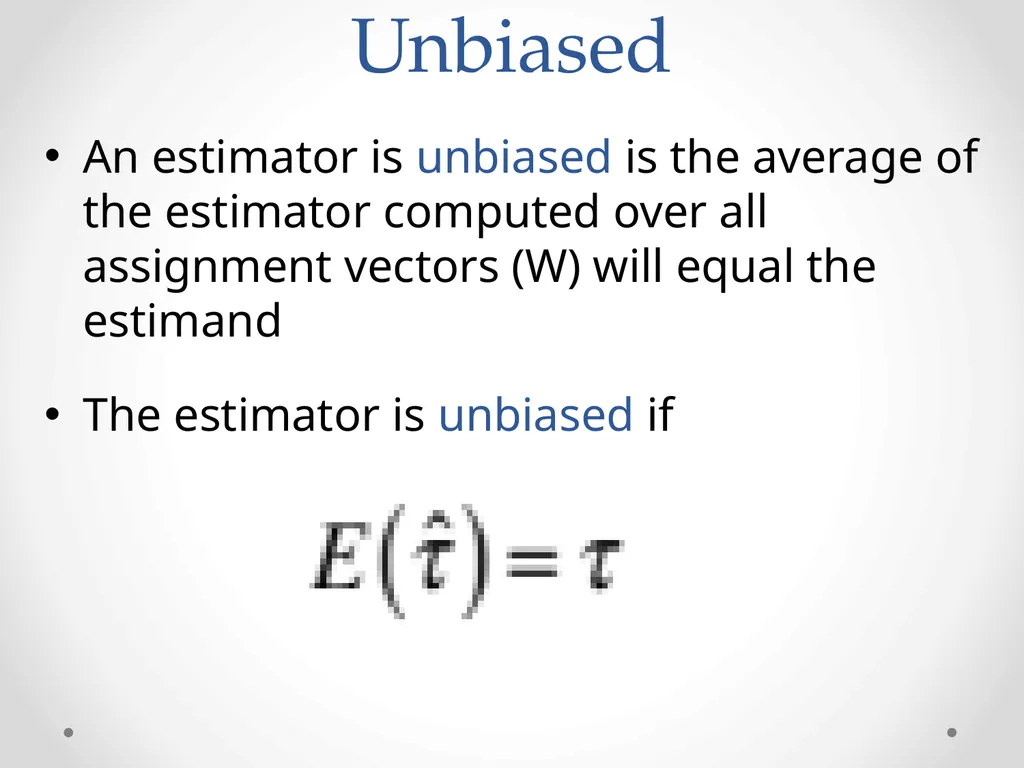
Unbiased An estimator is unbiased is the average of the estimator computed over all assignment vectors (W) will equal the estimand
The estimator is unbiased if<br>
17
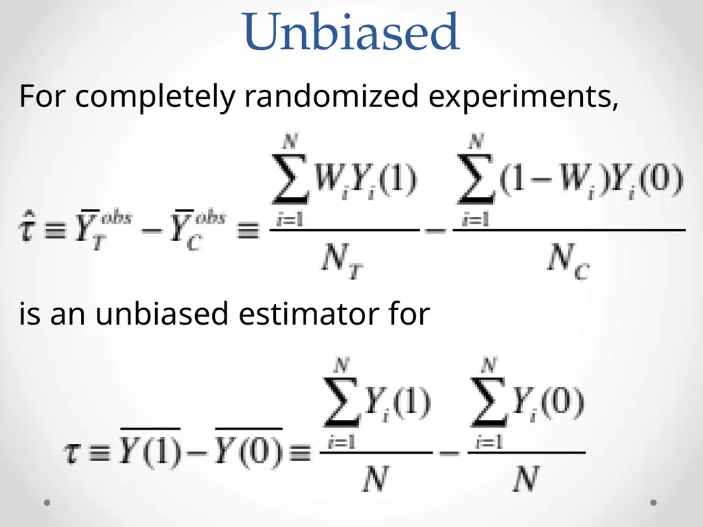
Unbiased For completely randomized experiments,
is an unbiased estimator for<br>
18
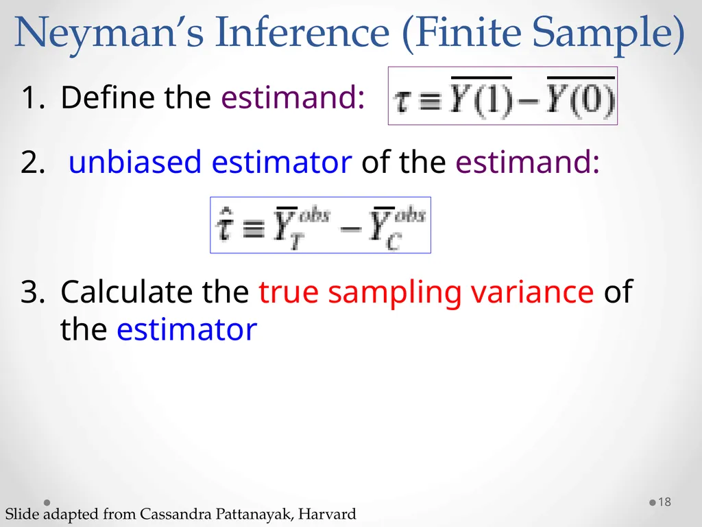
Neyman’s Inference (Finite Sample) Define the estimand:
unbiased estimator of the estimand:
Calculate the true sampling variance of the estimator 18 Slide adapted from Cassandra Pattanayak, Harvard<br>
19
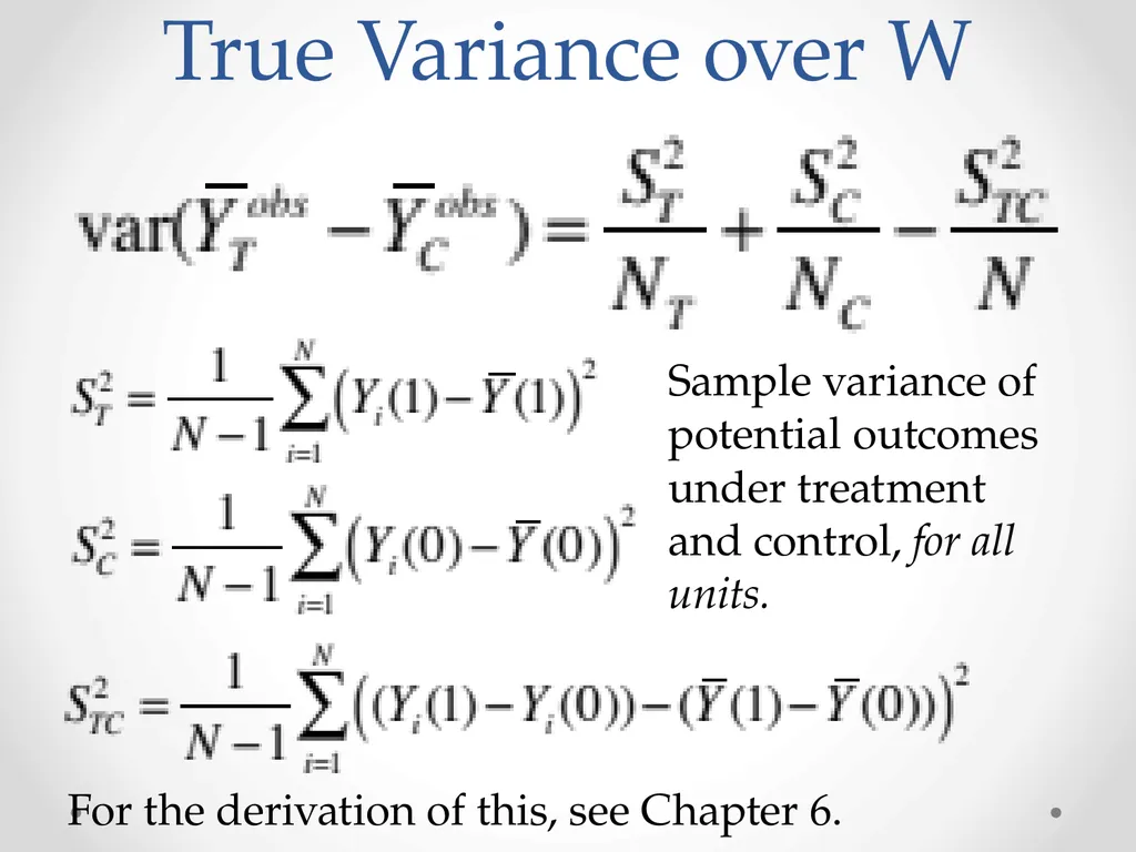
True Variance over W For the derivation of this, see Chapter 6. Sample variance of potential outcomes under treatment and control, for all units.<br>
20
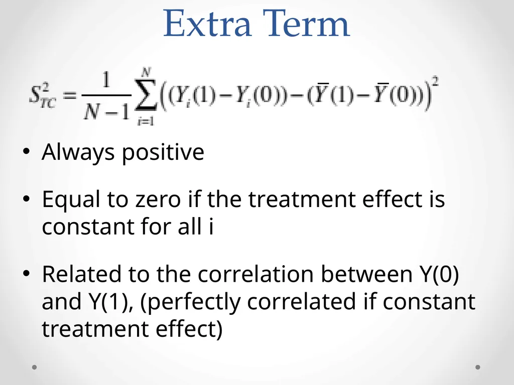
Extra Term Always positive
Equal to zero if the treatment effect is constant for all i
Related to the correlation between Y(0) and Y(1), (perfectly correlated if constant treatment effect)<br>
21
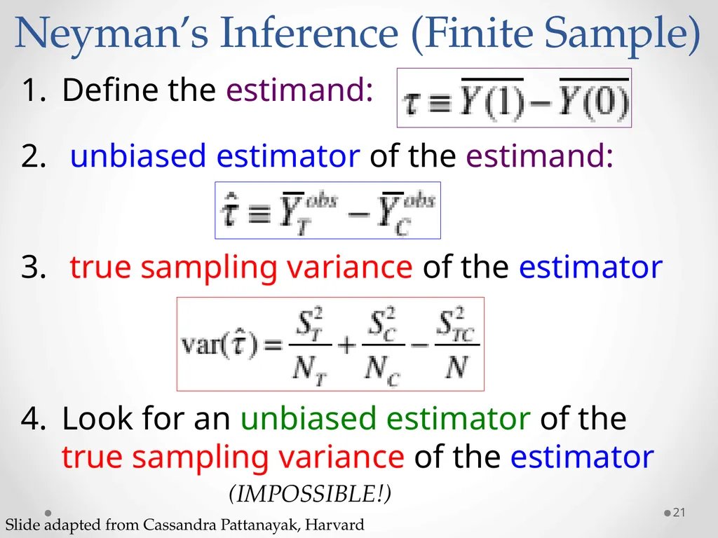
Neyman’s Inference (Finite Sample) Define the estimand:
unbiased estimator of the estimand:
true sampling variance of the estimator
Look for an unbiased estimator of the true sampling variance of the estimator 21 Slide adapted from Cassandra Pattanayak, Harvard (IMPOSSIBLE!)<br>
22
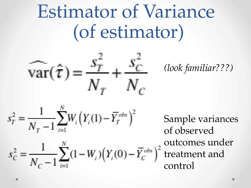
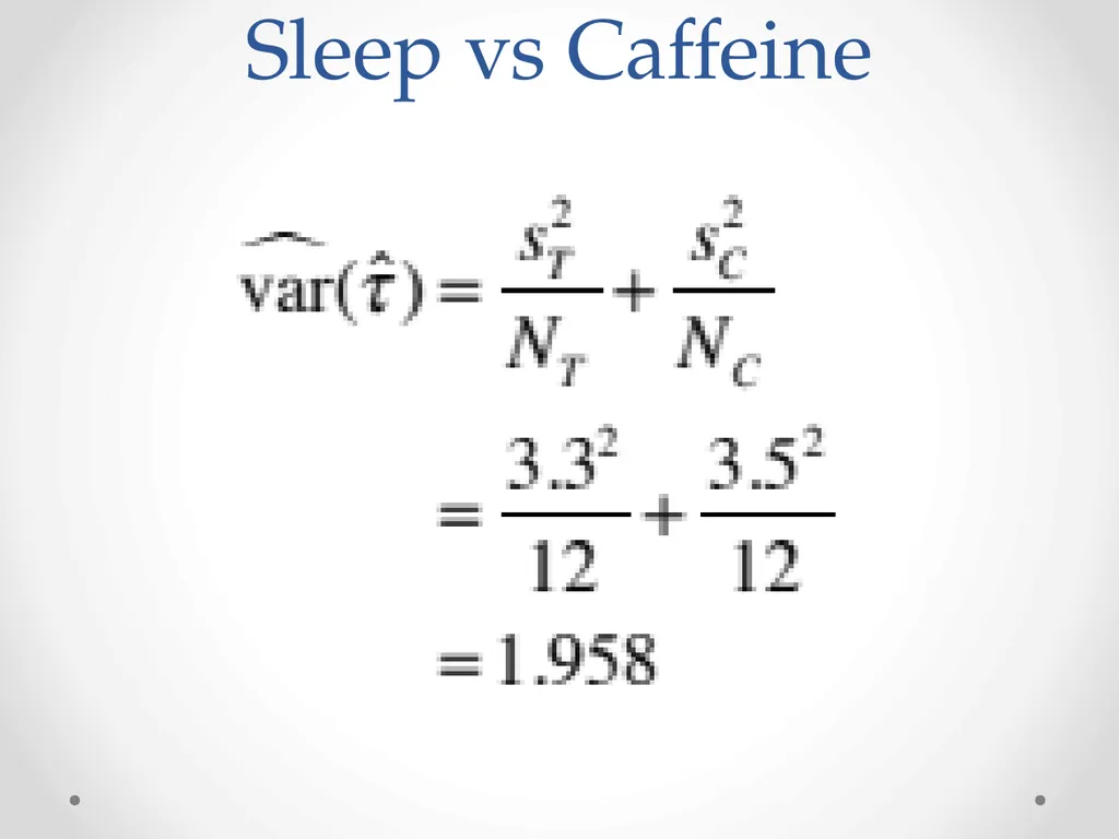
Estimator of Variance �(of estimator) Sample variances of observed outcomes under treatment and control (look familiar???)<br>
23
Estimator of Variance This is the standard variance estimate used in the familiar t-test
For finite samples, this is may be an overestimate of the true variance
Resulting inferences may be too conservative (confidence intervals will be too wide, p-values too large)<br>
25
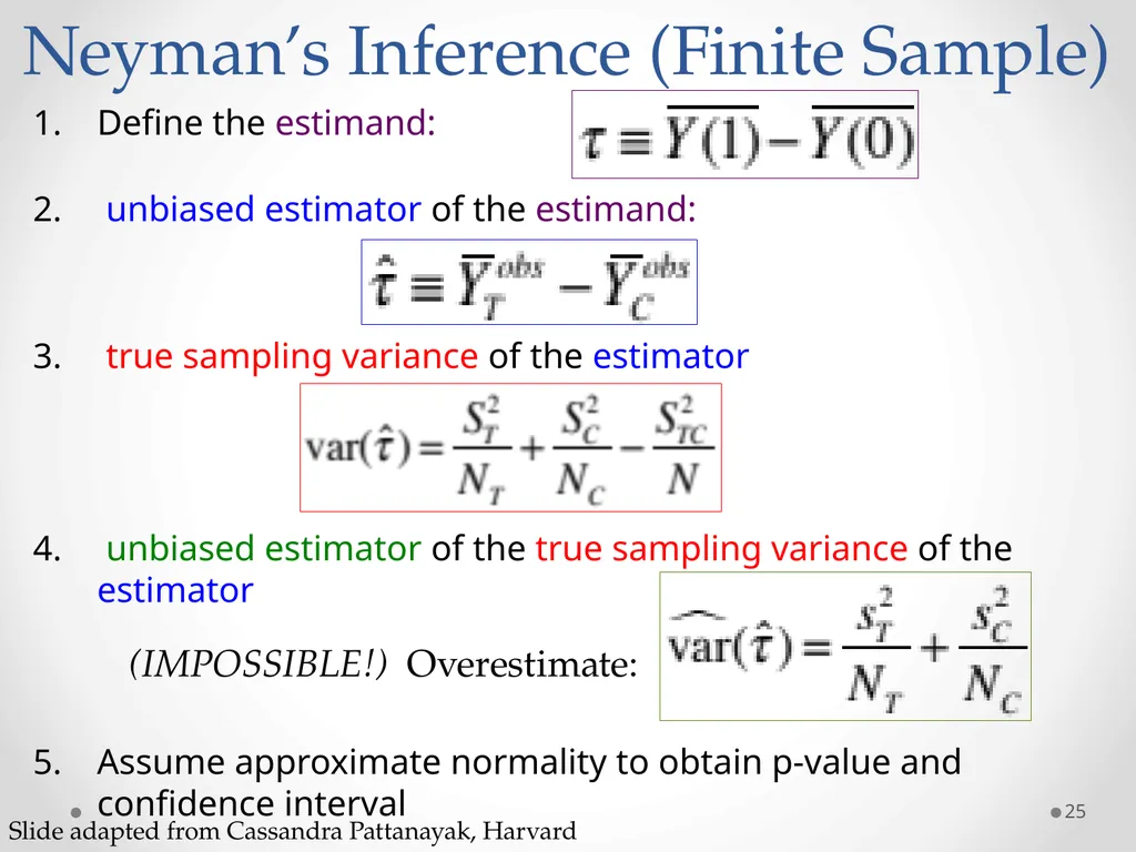
Neyman’s Inference (Finite Sample) Define the estimand:
unbiased estimator of the estimand:
true sampling variance of the estimator
unbiased estimator of the true sampling variance of the estimator
Assume approximate normality to obtain p-value and confidence interval 25 (IMPOSSIBLE!) Overestimate: Slide adapted from Cassandra Pattanayak, Harvard<br>
26
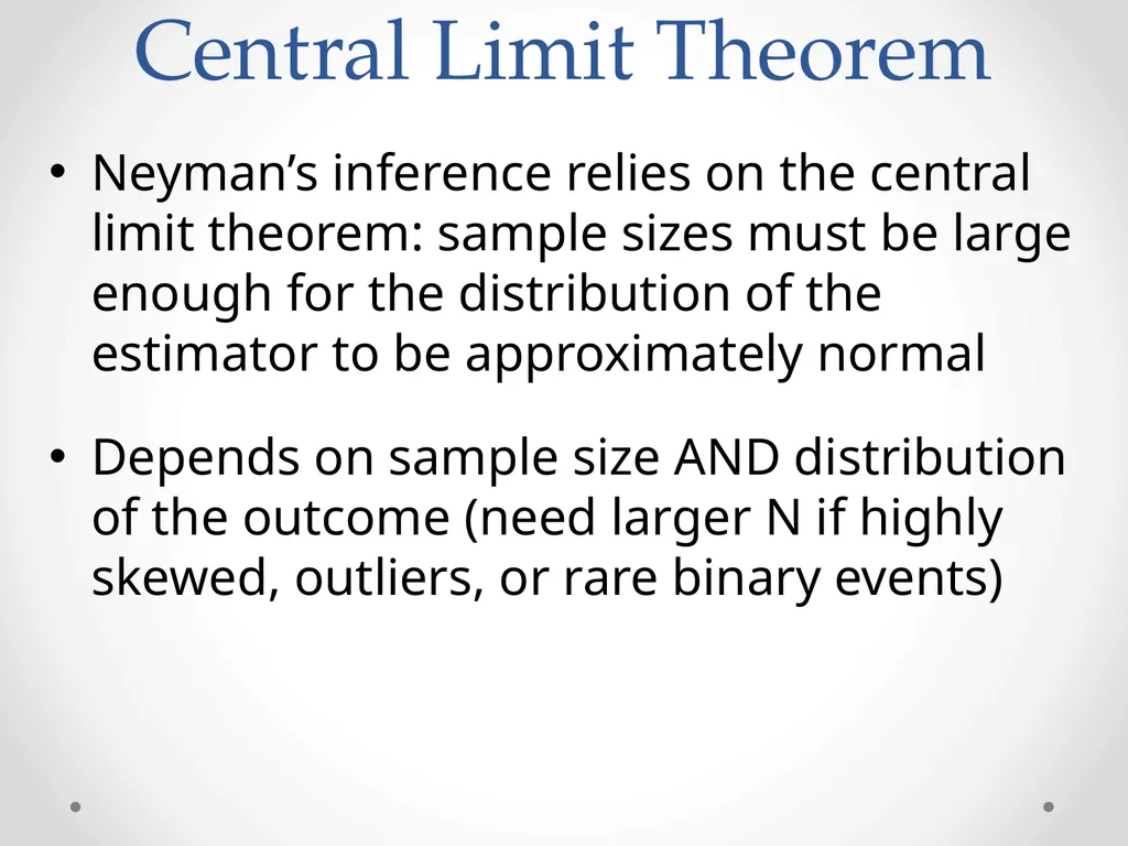
Central Limit Theorem Neyman’s inference relies on the central limit theorem: sample sizes must be large enough for the distribution of the estimator to be approximately normal
Depends on sample size AND distribution of the outcome (need larger N if highly skewed, outliers, or rare binary events)<br>
27
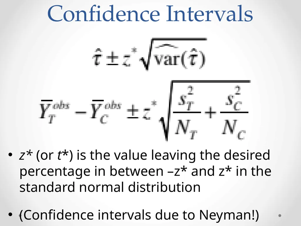
Confidence Intervals z* (or t*) is the value leaving the desired percentage in between –z* and z* in the standard normal distribution
(Confidence intervals due to Neyman!)<br>
28
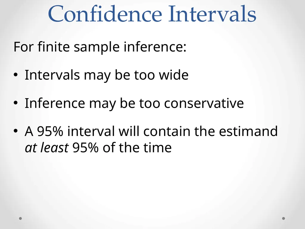
Confidence Intervals For finite sample inference:
Intervals may be too wide
Inference may be too conservative
A 95% interval will contain the estimand at least 95% of the time<br>
29
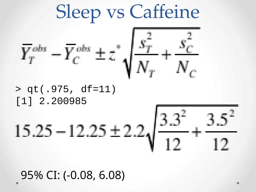
Sleep vs Caffeine > qt(.975, df=11)
[1] 2.200985 95% CI: (-0.08, 6.08)<br>
30
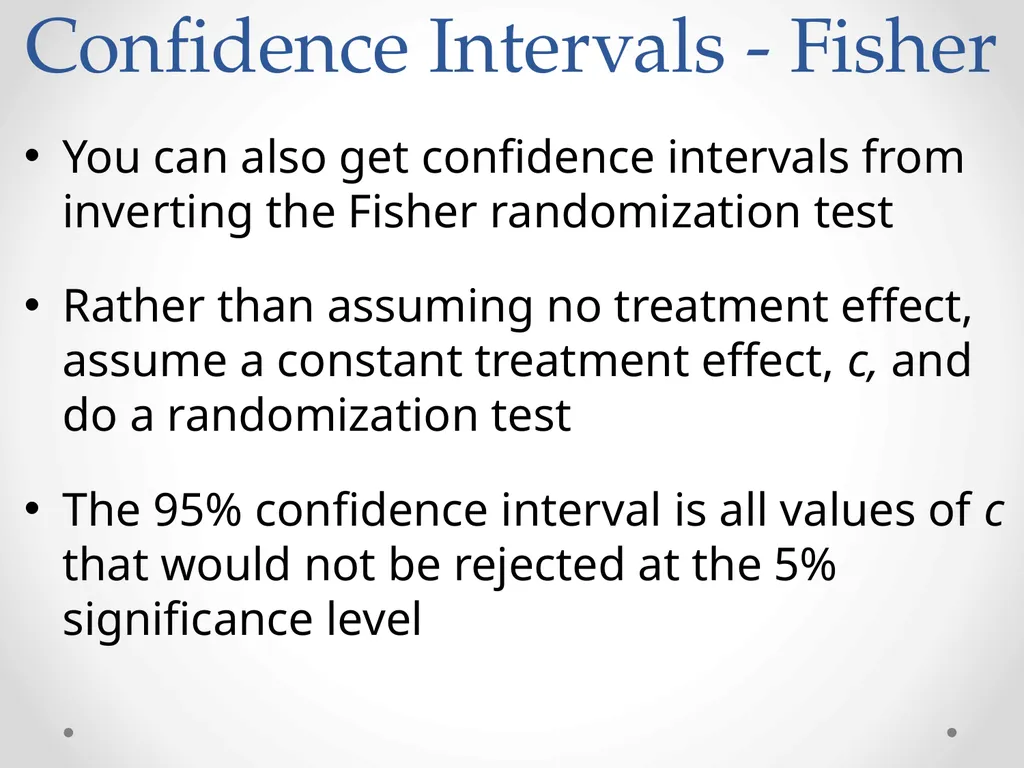
Confidence Intervals - Fisher You can also get confidence intervals from inverting the Fisher randomization test
Rather than assuming no treatment effect, assume a constant treatment effect, c, and do a randomization test
The 95% confidence interval is all values of c that would not be rejected at the 5% significance level<br>
31
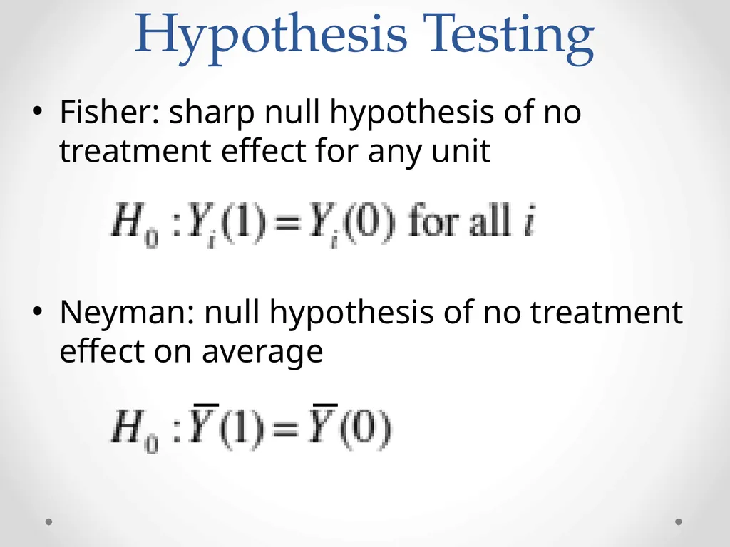
Hypothesis Testing Fisher: sharp null hypothesis of no treatment effect for any unit
Neyman: null hypothesis of no treatment effect on average<br>
32
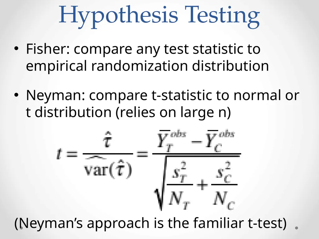
Hypothesis Testing Fisher: compare any test statistic to empirical randomization distribution
Neyman: compare t-statistic to normal or t distribution (relies on large n) (Neyman’s approach is the familiar t-test)<br>
33
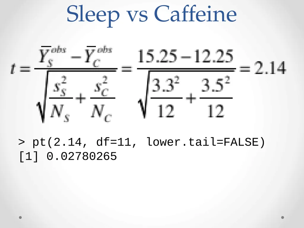
Sleep vs Caffeine > pt(2.14, df=11, lower.tail=FALSE)
[1] 0.02780265<br>
34
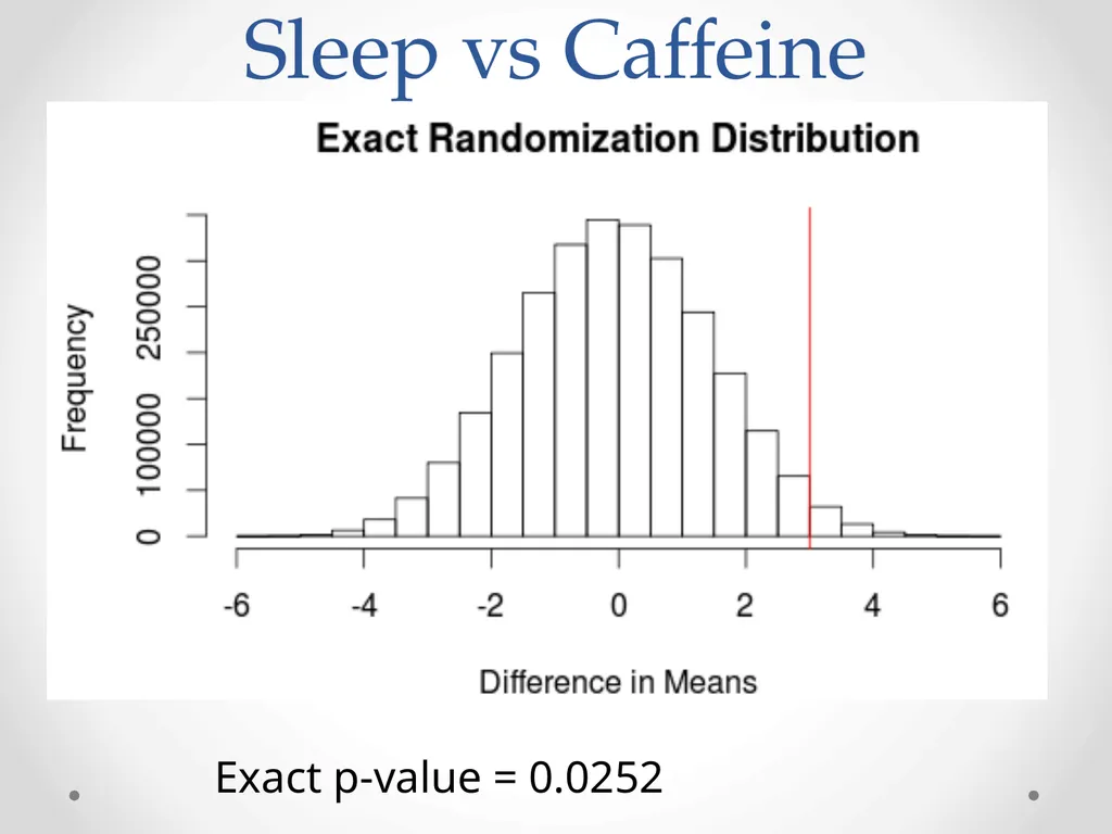
Sleep vs Caffeine Exact p-value = 0.0252<br>
35
Super Population Suppose we also want to consider random sampling from the population (in addition to random assignment)
How do things change?<br>
36
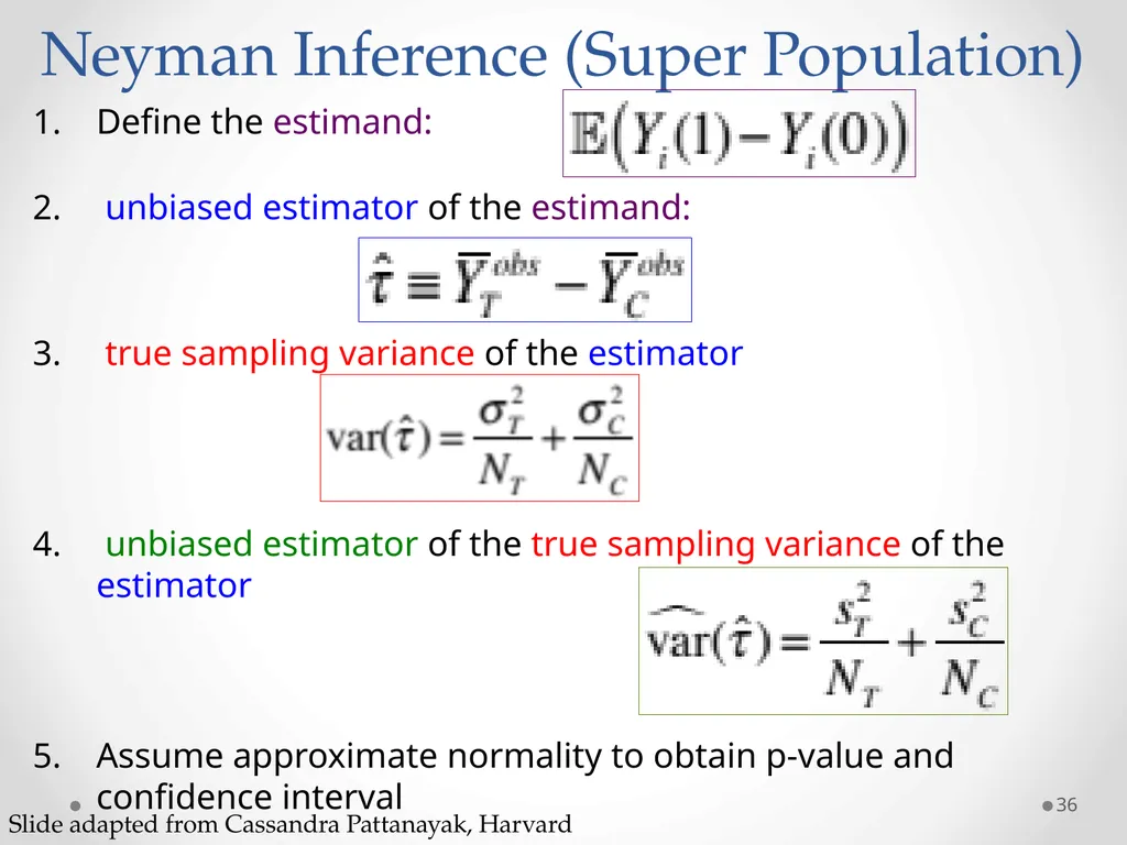
Neyman Inference (Super Population) Define the estimand:
unbiased estimator of the estimand:
true sampling variance of the estimator
unbiased estimator of the true sampling variance of the estimator
Assume approximate normality to obtain p-value and confidence interval 36 Slide adapted from Cassandra Pattanayak, Harvard<br>
37
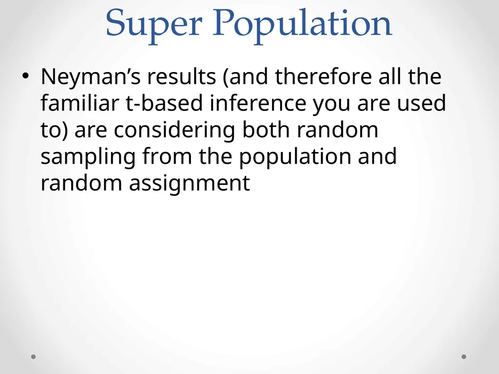
Super Population Neyman’s results (and therefore all the familiar t-based inference you are used to) are considering both random sampling from the population and random assignment<br>
39
To Do Read Ch 6
HW 2 due Monday 2/10<br>