
Introduction to Mediation Models with the PROCESS
CS
Published · 134 slides · 0 views

1 / 1











Description
Introduction to Mediation Models with the PROCESS Macro in SPSS Presented by Christine R. Wells, Ph.D. Statistical Methods and Data Analytics UCLA Office of Advanced Research Computing What we will cover in this workshop Some of what can be
Related Topics
Share
Embed code
Download this presentation From Below
"Introduction to Mediation Models with the PROCESS" is the property of its rightful owner. Permission is granted to download and print the materials on this website for personal, non-commercial use only, and to display it on your personal computer provided you do not modify the materials and that you retain all copyright notices contained in the materials. By downloading content from our website, you accept the terms of this agreement.
Presentation Transcript
01
Introduction to Mediation Models with the PROCESS Macro in SPSS Presented by Christine R. Wells, Ph.D.
Statistical Methods and Data Analytics
UCLA Office of Advanced Research Computing<br>
Statistical Methods and Data Analytics
UCLA Office of Advanced Research Computing<br>
02
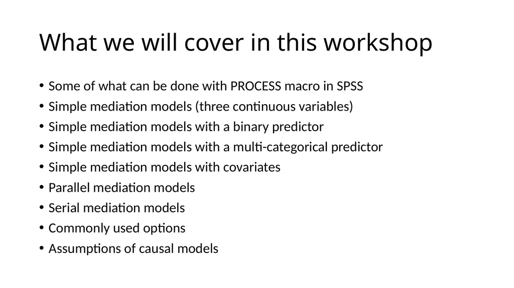
What we will cover in this workshop Some of what can be done with PROCESS macro in SPSS
Simple mediation models (three continuous variables)
Simple mediation models with a binary predictor
Simple mediation models with a multi-categorical predictor
Simple mediation models with covariates
Parallel mediation models
Serial mediation models
Commonly used options
Assumptions of causal models<br>
Simple mediation models (three continuous variables)
Simple mediation models with a binary predictor
Simple mediation models with a multi-categorical predictor
Simple mediation models with covariates
Parallel mediation models
Serial mediation models
Commonly used options
Assumptions of causal models<br>
03
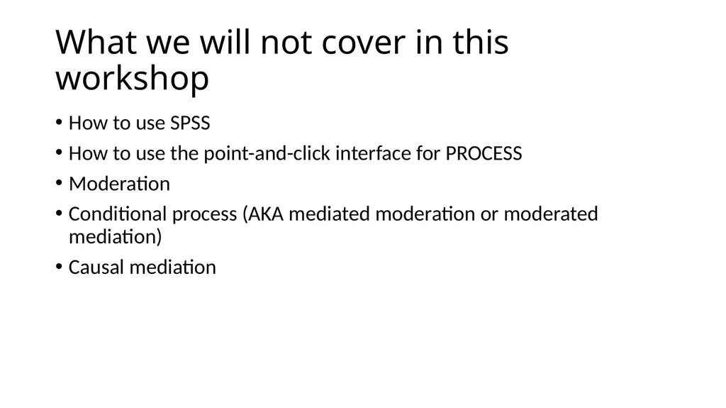
What we will not cover in this workshop How to use SPSS
How to use the point-and-click interface for PROCESS
Moderation
Conditional process (AKA mediated moderation or moderated mediation)
Causal mediation<br>
How to use the point-and-click interface for PROCESS
Moderation
Conditional process (AKA mediated moderation or moderated mediation)
Causal mediation<br>
04
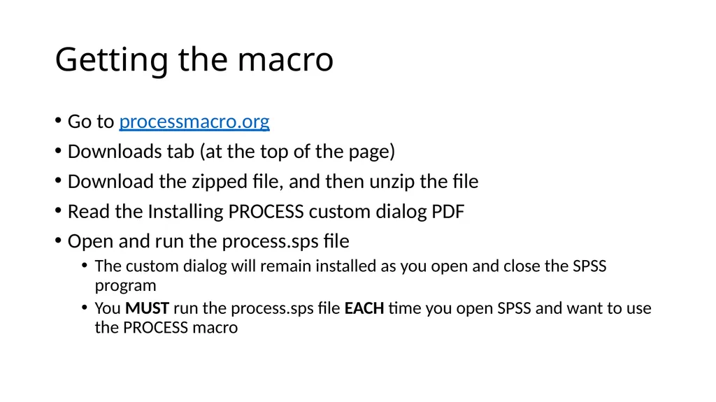
Getting the macro Go to processmacro.org
Downloads tab (at the top of the page)
Download the zipped file, and then unzip the file
Read the Installing PROCESS custom dialog PDF
Open and run the process.sps file
The custom dialog will remain installed as you open and close the SPSS program
You MUST run the process.sps file EACH time you open SPSS and want to use the PROCESS macro<br>
Downloads tab (at the top of the page)
Download the zipped file, and then unzip the file
Read the Installing PROCESS custom dialog PDF
Open and run the process.sps file
The custom dialog will remain installed as you open and close the SPSS program
You MUST run the process.sps file EACH time you open SPSS and want to use the PROCESS macro<br>
05
Where to find model numbers and more information Introduction to Mediation, Moderation and Conditional Process Analysis: A Regression-based Approach, Third Edition by Andrew F. Hayes (2022) Appendix A
New edition of both the macro and the book expected in 2025
Go to https://haskayne.ucalgary.ca/CCRAM/resource-hub to watch a video describing the new features (about half way down the page)<br>
New edition of both the macro and the book expected in 2025
Go to https://haskayne.ucalgary.ca/CCRAM/resource-hub to watch a video describing the new features (about half way down the page)<br>
06
Linear regression Linear regression (AKA OLS) is the foundation of mediation
OLS gives the relationship between X (the predictor) and Y (the outcome)
Relationship is a general term that could be
Correlational
Causal
Other
The analysis cannot tell you the nature of the relationship!<br>
OLS gives the relationship between X (the predictor) and Y (the outcome)
Relationship is a general term that could be
Correlational
Causal
Other
The analysis cannot tell you the nature of the relationship!<br>
07
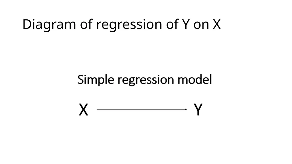
Diagram of regression of Y on X<br>
08
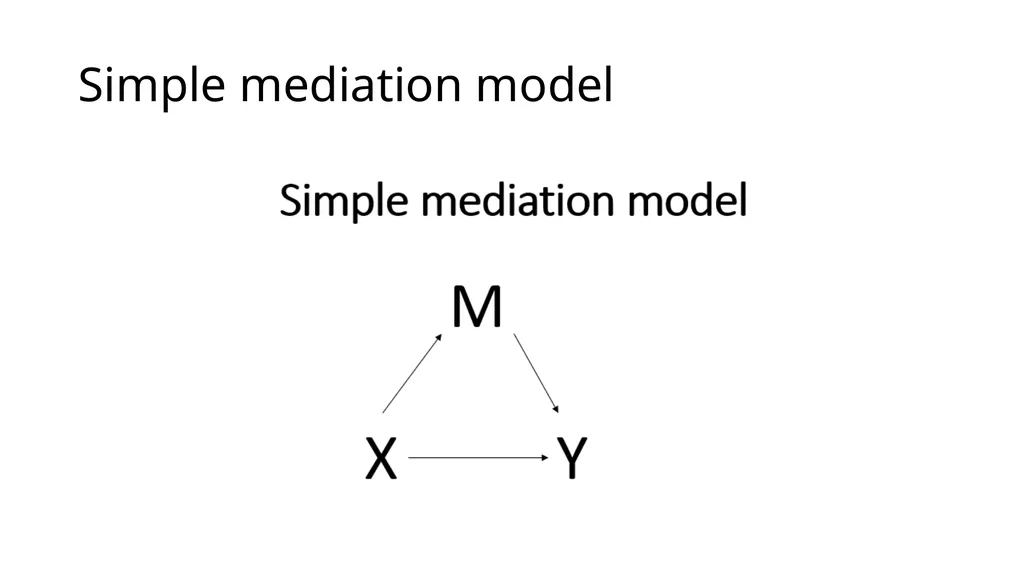
Simple mediation model with continuous predictor Mediation includes a variable between X and Y
Called M (the mediator)
Mathematically, the mediator acts like a covariate in the model
Conceptually, the mediator changes the simple regression model from a model that looks at the association of two variables to a model that tries to look at a causal relationship<br>
Called M (the mediator)
Mathematically, the mediator acts like a covariate in the model
Conceptually, the mediator changes the simple regression model from a model that looks at the association of two variables to a model that tries to look at a causal relationship<br>
09
Simple mediation model<br>
10
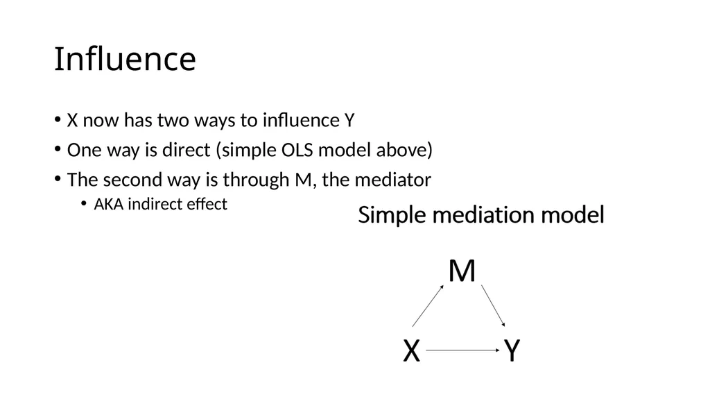
Influence X now has two ways to influence Y
One way is direct (simple OLS model above)
The second way is through M, the mediator
AKA indirect effect<br>
One way is direct (simple OLS model above)
The second way is through M, the mediator
AKA indirect effect<br>
11
Vocabulary Antecents: come before something else
X is an antecent of Y
Consequent variable: consequence of the process the model describes
Y is the consequent variable<br>
X is an antecent of Y
Consequent variable: consequence of the process the model describes
Y is the consequent variable<br>
12
Questions Why use PROCESS or other special software or procedures if mediation is just regression?
Or is it just regression?
Is M (the mediator) an antecedent variable or a consequent variable?<br>
Or is it just regression?
Is M (the mediator) an antecedent variable or a consequent variable?<br>
13
Answers Much of the output given by PROCESS can be obtained from SPSS’s regression commands
But some of the necessary output cannot
Even if we can calculate some values from the regression output, we want PROCESS to calculate standard errors for us
M is both an antecent and a consequent variable!<br>
But some of the necessary output cannot
Even if we can calculate some values from the regression output, we want PROCESS to calculate standard errors for us
M is both an antecent and a consequent variable!<br>
14
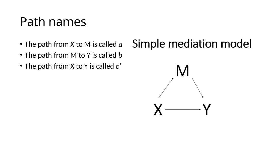
Path names The path from X to M is called a
The path from M to Y is called b
The path from X to Y is called c’<br>
The path from M to Y is called b
The path from X to Y is called c’<br>
15
Calculating the indirect and total effects The indirect effect of X on Y through M is obtained by multiplying the a-path coefficient and b-path coefficient
The total effect (called c) is the sum of the direct effect and the indirect effect: c = (a * b) + c’<br>
The total effect (called c) is the sum of the direct effect and the indirect effect: c = (a * b) + c’<br>
16
When to use normal theory versus bootstrap? Normal theory is OK for most of the tests of statistical significance
Bootstrap is usually necessary for the test of indirect effects
Indirect effect is the product of the a-path coefficient and the b-path coefficient
The sampling distribution of a product term is usually not normally distributed
Using standard errors based on normal theory may have lower than other approaches<br>
Bootstrap is usually necessary for the test of indirect effects
Indirect effect is the product of the a-path coefficient and the b-path coefficient
The sampling distribution of a product term is usually not normally distributed
Using standard errors based on normal theory may have lower than other approaches<br>
17
Types of variables that can be used in PROCESS The outcome and mediator must be continuous when using the PROCESS macro
PROCESS checks for this and will not run if these variables are not continuous
The predictor may be continuous, binary or have multiple categories
Important: Variable names should be eight characters or shorter!<br>
PROCESS checks for this and will not run if these variables are not continuous
The predictor may be continuous, binary or have multiple categories
Important: Variable names should be eight characters or shorter!<br>
18
Example dataset The example dataset is hsbmediation
Contains 200 observations from a fictional study
Researchers randomly assigned participants to receive information about senior living facilities
The amount of detail given to participants ranged from a little to quite a lot along a continuous scale (called detail in the dataset) and is the predictor, or X
The mediator (M) was the feeling of the participants (the variable feeling in the dataset)
The outcome (Y) was a measure of opinion strength regarding a proposed change to a law regarding senior living facilities (opinion in the dataset)<br>
Contains 200 observations from a fictional study
Researchers randomly assigned participants to receive information about senior living facilities
The amount of detail given to participants ranged from a little to quite a lot along a continuous scale (called detail in the dataset) and is the predictor, or X
The mediator (M) was the feeling of the participants (the variable feeling in the dataset)
The outcome (Y) was a measure of opinion strength regarding a proposed change to a law regarding senior living facilities (opinion in the dataset)<br>
19
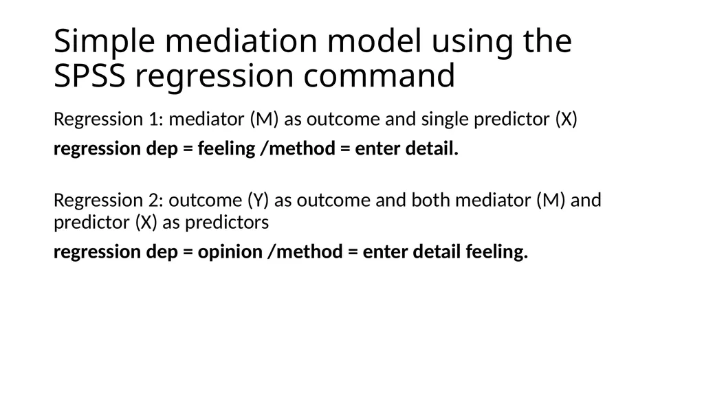
Simple mediation model using the SPSS regression command Regression 1: mediator (M) as outcome and single predictor (X)
regression dep = feeling /method = enter detail.
Regression 2: outcome (Y) as outcome and both mediator (M) and predictor (X) as predictors
regression dep = opinion /method = enter detail feeling.<br>
regression dep = feeling /method = enter detail.
Regression 2: outcome (Y) as outcome and both mediator (M) and predictor (X) as predictors
regression dep = opinion /method = enter detail feeling.<br>
20
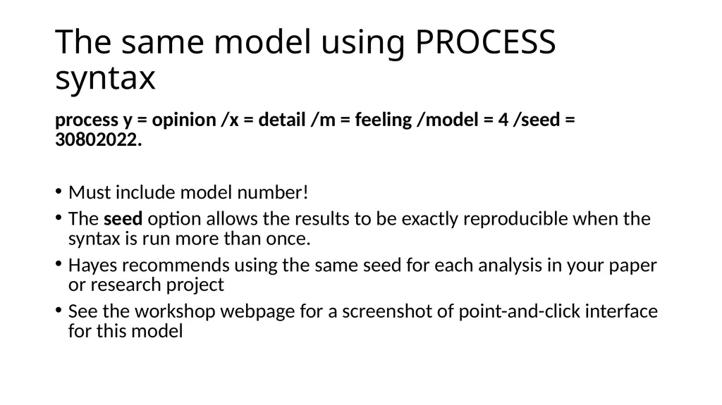
The same model using PROCESS syntax process y = opinion /x = detail /m = feeling /model = 4 /seed = 30802022.
Must include model number!
The seed option allows the results to be exactly reproducible when the syntax is run more than once.
Hayes recommends using the same seed for each analysis in your paper or research project
See the workshop webpage for a screenshot of point-and-click interface for this model<br>
Must include model number!
The seed option allows the results to be exactly reproducible when the syntax is run more than once.
Hayes recommends using the same seed for each analysis in your paper or research project
See the workshop webpage for a screenshot of point-and-click interface for this model<br>
21
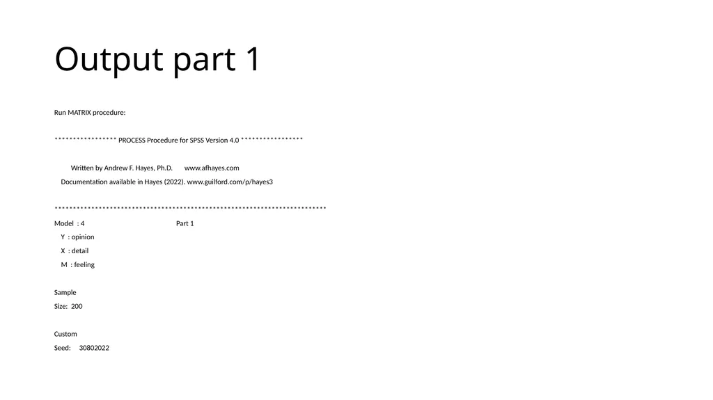
Output part 1 Run MATRIX procedure:
***************** PROCESS Procedure for SPSS Version 4.0 *****************
Written by Andrew F. Hayes, Ph.D. www.afhayes.com
Documentation available in Hayes (2022). www.guilford.com/p/hayes3
**************************************************************************
Model : 4 Part 1
Y : opinion
X : detail
M : feeling
Sample
Size: 200
Custom
Seed: 30802022<br>
***************** PROCESS Procedure for SPSS Version 4.0 *****************
Written by Andrew F. Hayes, Ph.D. www.afhayes.com
Documentation available in Hayes (2022). www.guilford.com/p/hayes3
**************************************************************************
Model : 4 Part 1
Y : opinion
X : detail
M : feeling
Sample
Size: 200
Custom
Seed: 30802022<br>
22
Output part 1 continued Check this before moving on!
Ensures clear communication between you and PROCESS<br>
Ensures clear communication between you and PROCESS<br>
23
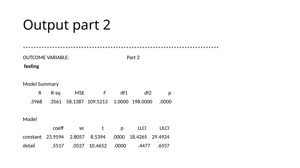
Output part 2 **************************************************************************
OUTCOME VARIABLE: Part 2
feeling
Model Summary
R R-sq MSE F df1 df2 p
.5968 .3561 58.1387 109.5213 1.0000 198.0000 .0000
Model
coeff se t p LLCI ULCI
constant 23.9594 2.8057 8.5394 .0000 18.4265 29.4924
detail .5517 .0527 10.4652 .0000 .4477 .6557<br>
OUTCOME VARIABLE: Part 2
feeling
Model Summary
R R-sq MSE F df1 df2 p
.5968 .3561 58.1387 109.5213 1.0000 198.0000 .0000
Model
coeff se t p LLCI ULCI
constant 23.9594 2.8057 8.5394 .0000 18.4265 29.4924
detail .5517 .0527 10.4652 .0000 .4477 .6557<br>
24
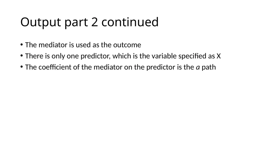
Output part 2 continued The mediator is used as the outcome
There is only one predictor, which is the variable specified as X
The coefficient of the mediator on the predictor is the a path<br>
There is only one predictor, which is the variable specified as X
The coefficient of the mediator on the predictor is the a path<br>
25
Output part 2 continued A generic interpretation is that “… for two cases that are equal on M but differ by one unit on X, c’ is the estimated value of Y for the case with X = x minus the estimated value of Y for the case with X = x – 1.…the sign of c’ tells whether the case one unit higher on X is estimated to be higher (c’ = +) or lower (c’ = -) on Y. So a positive direct effect means that the case higher on X is estimated to be higher on Y, whereas a negative direct effect means that the case higher on X is estimated to be lower on Y.<br>
26
Output part 2 continued In the special case where X is dichotomous, with the two values of X differing by a single unit (e.g., X = 1 and X = 0), Y-hat can be interpreted as a group mean, …, meaning it estimates the difference between the two group means holding M constant. This is equivalent to what in analysis of covariance terms is called an adjusted mean difference” (page 85).<br>
27
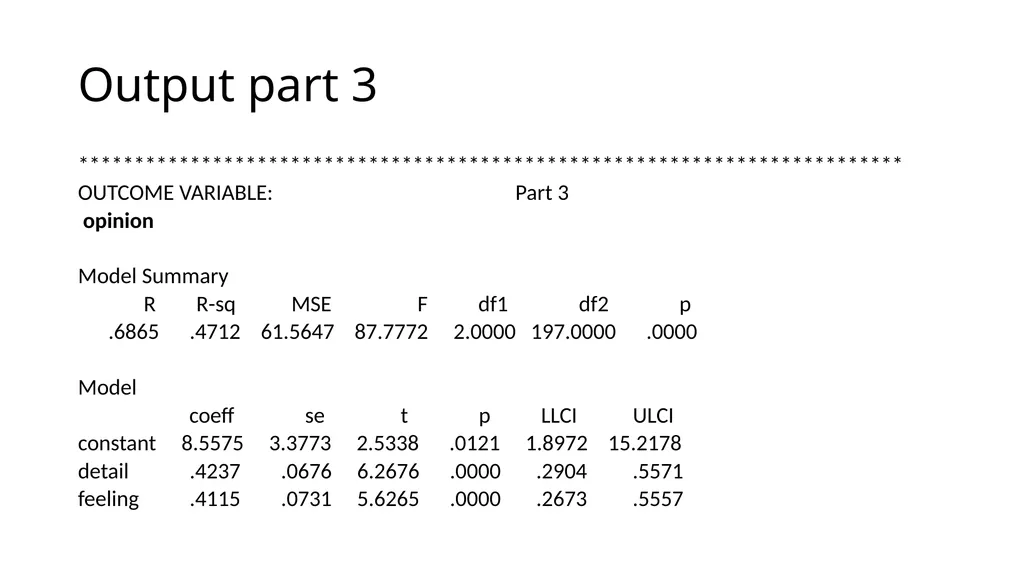
Output part 3 **************************************************************************
OUTCOME VARIABLE: Part 3
opinion
Model Summary
R R-sq MSE F df1 df2 p
.6865 .4712 61.5647 87.7772 2.0000 197.0000 .0000
Model
coeff se t p LLCI ULCI
constant 8.5575 3.3773 2.5338 .0121 1.8972 15.2178
detail .4237 .0676 6.2676 .0000 .2904 .5571
feeling .4115 .0731 5.6265 .0000 .2673 .5557<br>
OUTCOME VARIABLE: Part 3
opinion
Model Summary
R R-sq MSE F df1 df2 p
.6865 .4712 61.5647 87.7772 2.0000 197.0000 .0000
Model
coeff se t p LLCI ULCI
constant 8.5575 3.3773 2.5338 .0121 1.8972 15.2178
detail .4237 .0676 6.2676 .0000 .2904 .5571
feeling .4115 .0731 5.6265 .0000 .2673 .5557<br>
28
Output part 3 continued Y is used as the outcome variable, and X and M are predictors
This output gives the b and c’ paths
The interpretation of b is the same as the interpretation of a, except that M is the antecedent instead of X, and Y is the outcome
“Two cases that differ by one unit on M but that are equal on X are estimated to differ by b units on Y” (page 86)<br>
This output gives the b and c’ paths
The interpretation of b is the same as the interpretation of a, except that M is the antecedent instead of X, and Y is the outcome
“Two cases that differ by one unit on M but that are equal on X are estimated to differ by b units on Y” (page 86)<br>
29
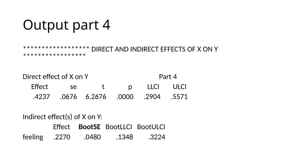
Output part 4 ****************** DIRECT AND INDIRECT EFFECTS OF X ON Y *****************
Direct effect of X on Y Part 4
Effect se t p LLCI ULCI
.4237 .0676 6.2676 .0000 .2904 .5571
Indirect effect(s) of X on Y:
Effect BootSE BootLLCI BootULCI
feeling .2270 .0480 .1348 .3224<br>
Direct effect of X on Y Part 4
Effect se t p LLCI ULCI
.4237 .0676 6.2676 .0000 .2904 .5571
Indirect effect(s) of X on Y:
Effect BootSE BootLLCI BootULCI
feeling .2270 .0480 .1348 .3224<br>
30
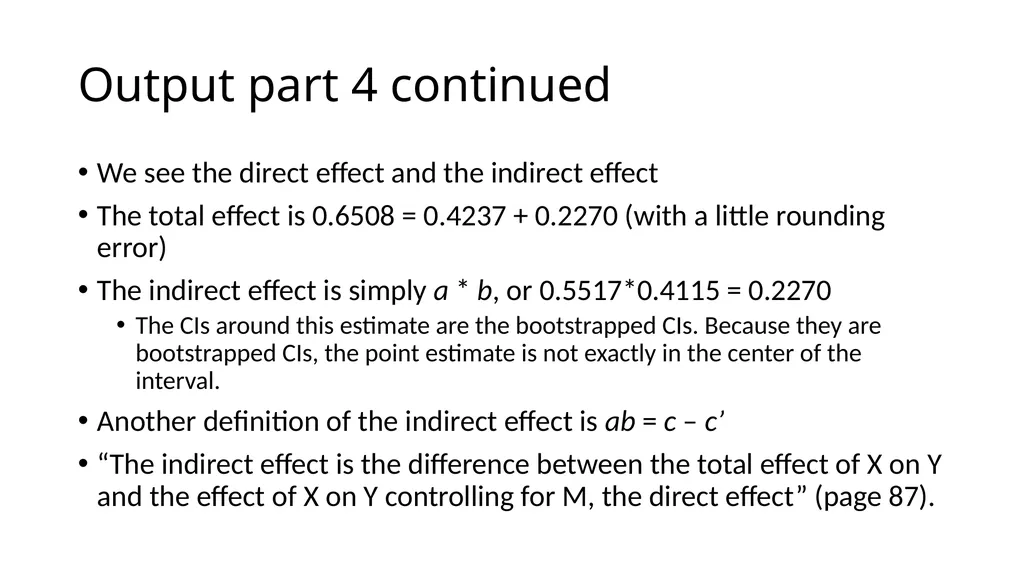
Output part 4 continued We see the direct effect and the indirect effect
The total effect is 0.6508 = 0.4237 + 0.2270 (with a little rounding error)
The indirect effect is simply a * b, or 0.5517*0.4115 = 0.2270
The CIs around this estimate are the bootstrapped CIs. Because they are bootstrapped CIs, the point estimate is not exactly in the center of the interval.
Another definition of the indirect effect is ab = c – c’
“The indirect effect is the difference between the total effect of X on Y and the effect of X on Y controlling for M, the direct effect” (page 87).<br>
The total effect is 0.6508 = 0.4237 + 0.2270 (with a little rounding error)
The indirect effect is simply a * b, or 0.5517*0.4115 = 0.2270
The CIs around this estimate are the bootstrapped CIs. Because they are bootstrapped CIs, the point estimate is not exactly in the center of the interval.
Another definition of the indirect effect is ab = c – c’
“The indirect effect is the difference between the total effect of X on Y and the effect of X on Y controlling for M, the direct effect” (page 87).<br>
31
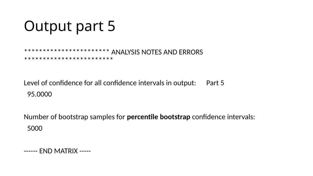
Output part 5 *********************** ANALYSIS NOTES AND ERRORS ************************
Level of confidence for all confidence intervals in output: Part 5
95.0000
Number of bootstrap samples for percentile bootstrap confidence intervals:
5000
------ END MATRIX -----<br>
Level of confidence for all confidence intervals in output: Part 5
95.0000
Number of bootstrap samples for percentile bootstrap confidence intervals:
5000
------ END MATRIX -----<br>
32
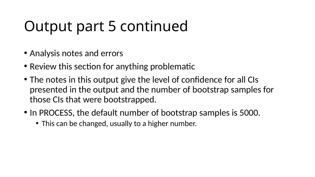
Output part 5 continued Analysis notes and errors
Review this section for anything problematic
The notes in this output give the level of confidence for all CIs presented in the output and the number of bootstrap samples for those CIs that were bootstrapped.
In PROCESS, the default number of bootstrap samples is 5000.
This can be changed, usually to a higher number.<br>
Review this section for anything problematic
The notes in this output give the level of confidence for all CIs presented in the output and the number of bootstrap samples for those CIs that were bootstrapped.
In PROCESS, the default number of bootstrap samples is 5000.
This can be changed, usually to a higher number.<br>
33
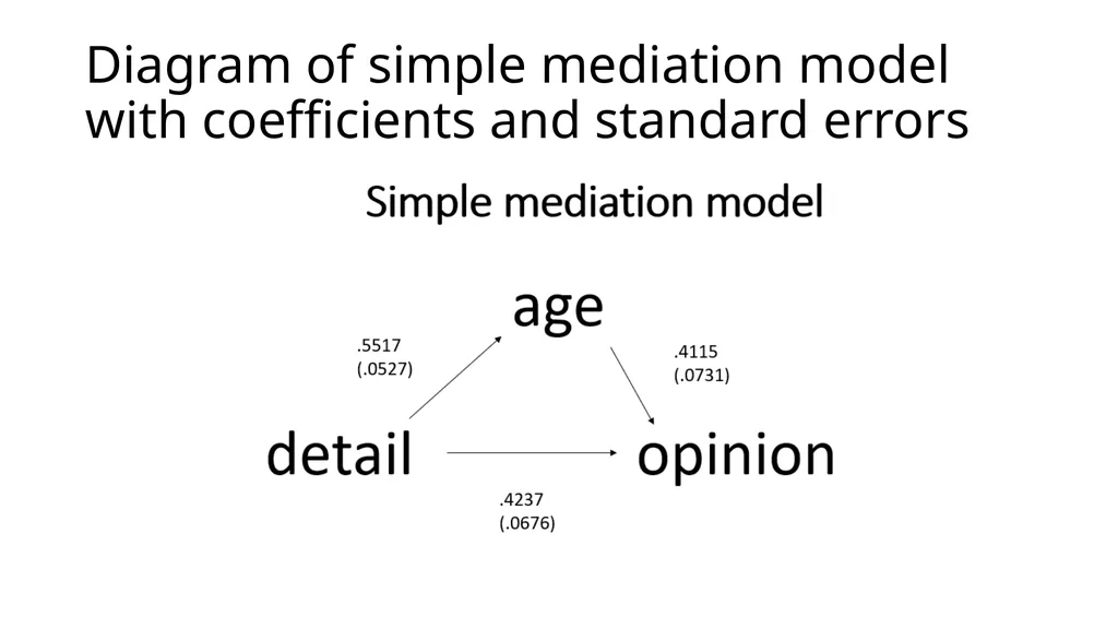
Diagram of simple mediation model with coefficients and standard errors<br>
34
Question Can you confirm the calculations for the indirect and total effects?<br>
35
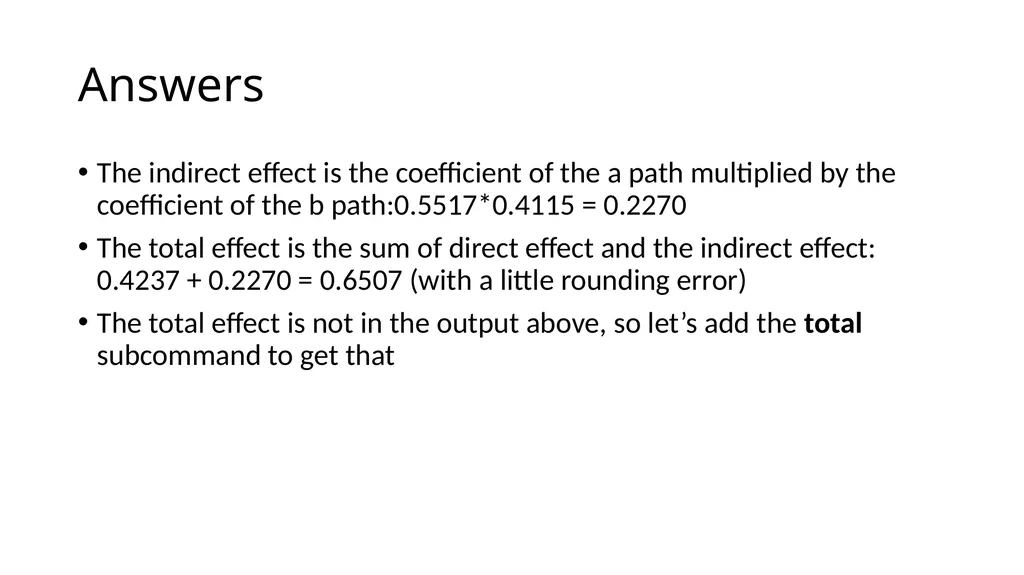
Answers The indirect effect is the coefficient of the a path multiplied by the coefficient of the b path:0.5517*0.4115 = 0.2270
The total effect is the sum of direct effect and the indirect effect: 0.4237 + 0.2270 = 0.6507 (with a little rounding error)
The total effect is not in the output above, so let’s add the total subcommand to get that<br>
The total effect is the sum of direct effect and the indirect effect: 0.4237 + 0.2270 = 0.6507 (with a little rounding error)
The total effect is not in the output above, so let’s add the total subcommand to get that<br>
36
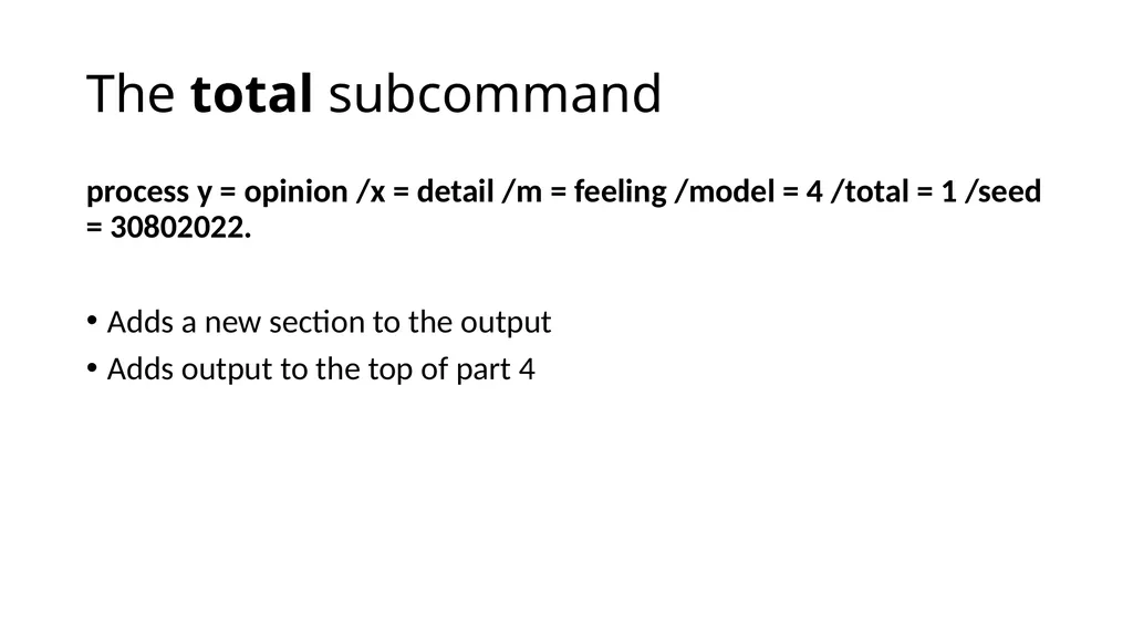
The total subcommand process y = opinion /x = detail /m = feeling /model = 4 /total = 1 /seed = 30802022.
Adds a new section to the output
Adds output to the top of part 4<br>
Adds a new section to the output
Adds output to the top of part 4<br>
37
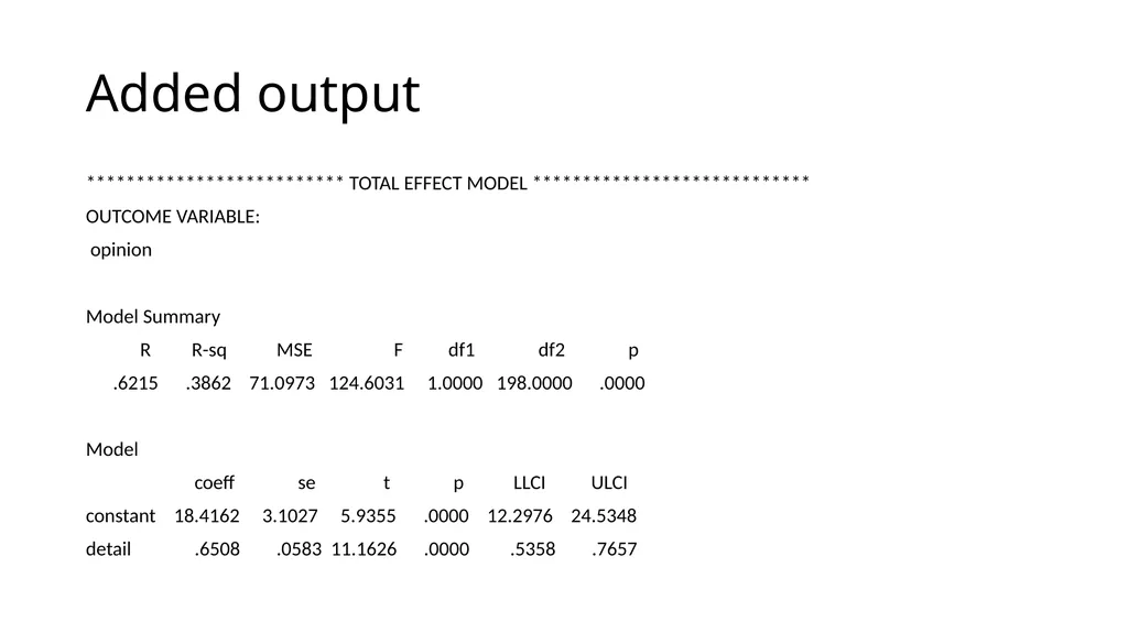
Added output ************************** TOTAL EFFECT MODEL ****************************
OUTCOME VARIABLE:
opinion
Model Summary
R R-sq MSE F df1 df2 p
.6215 .3862 71.0973 124.6031 1.0000 198.0000 .0000
Model
coeff se t p LLCI ULCI
constant 18.4162 3.1027 5.9355 .0000 12.2976 24.5348
detail .6508 .0583 11.1626 .0000 .5358 .7657<br>
OUTCOME VARIABLE:
opinion
Model Summary
R R-sq MSE F df1 df2 p
.6215 .3862 71.0973 124.6031 1.0000 198.0000 .0000
Model
coeff se t p LLCI ULCI
constant 18.4162 3.1027 5.9355 .0000 12.2976 24.5348
detail .6508 .0583 11.1626 .0000 .5358 .7657<br>
38
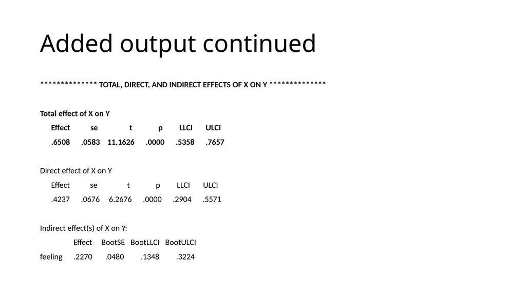
Added output continued ************** TOTAL, DIRECT, AND INDIRECT EFFECTS OF X ON Y **************
Total effect of X on Y
Effect se t p LLCI ULCI
.6508 .0583 11.1626 .0000 .5358 .7657
Direct effect of X on Y
Effect se t p LLCI ULCI
.4237 .0676 6.2676 .0000 .2904 .5571
Indirect effect(s) of X on Y:
Effect BootSE BootLLCI BootULCI
feeling .2270 .0480 .1348 .3224<br>
Total effect of X on Y
Effect se t p LLCI ULCI
.6508 .0583 11.1626 .0000 .5358 .7657
Direct effect of X on Y
Effect se t p LLCI ULCI
.4237 .0676 6.2676 .0000 .2904 .5571
Indirect effect(s) of X on Y:
Effect BootSE BootLLCI BootULCI
feeling .2270 .0480 .1348 .3224<br>
39
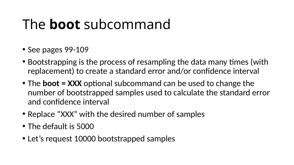
The boot subcommand See pages 99-109
Bootstrapping is the process of resampling the data many times (with replacement) to create a standard error and/or confidence interval
The boot = XXX optional subcommand can be used to change the number of bootstrapped samples used to calculate the standard error and confidence interval
Replace “XXX” with the desired number of samples
The default is 5000
Let’s request 10000 bootstrapped samples<br>
Bootstrapping is the process of resampling the data many times (with replacement) to create a standard error and/or confidence interval
The boot = XXX optional subcommand can be used to change the number of bootstrapped samples used to calculate the standard error and confidence interval
Replace “XXX” with the desired number of samples
The default is 5000
Let’s request 10000 bootstrapped samples<br>
40
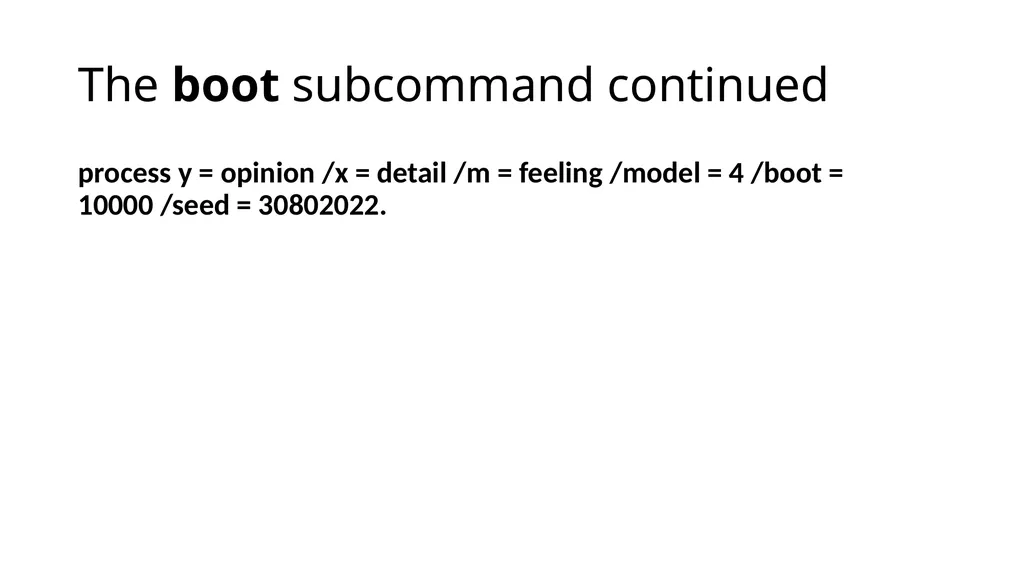
The boot subcommand continued process y = opinion /x = detail /m = feeling /model = 4 /boot = 10000 /seed = 30802022.<br>
41
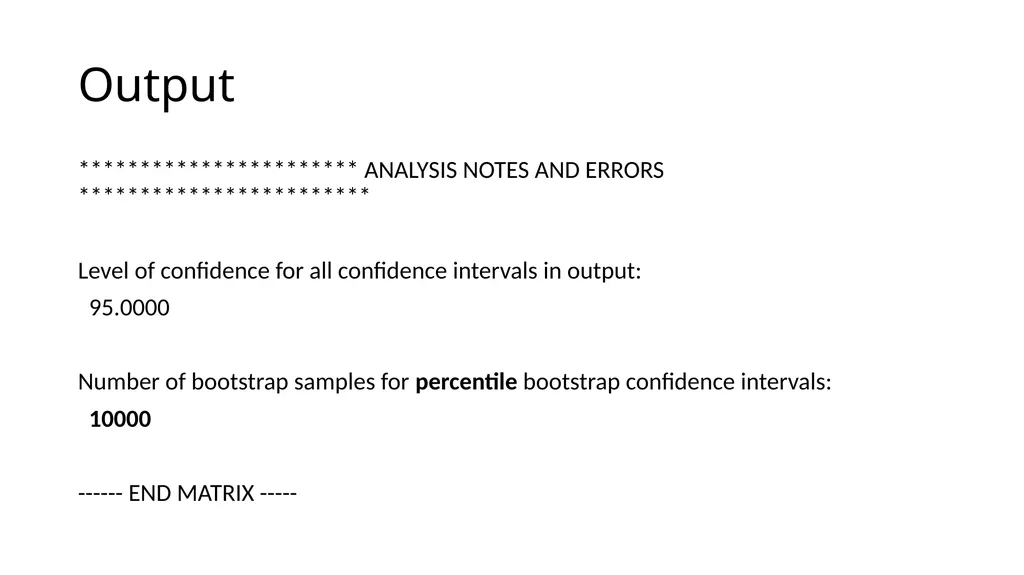
Output *********************** ANALYSIS NOTES AND ERRORS ************************
Level of confidence for all confidence intervals in output:
95.0000
Number of bootstrap samples for percentile bootstrap confidence intervals:
10000
------ END MATRIX -----<br>
Level of confidence for all confidence intervals in output:
95.0000
Number of bootstrap samples for percentile bootstrap confidence intervals:
10000
------ END MATRIX -----<br>
42
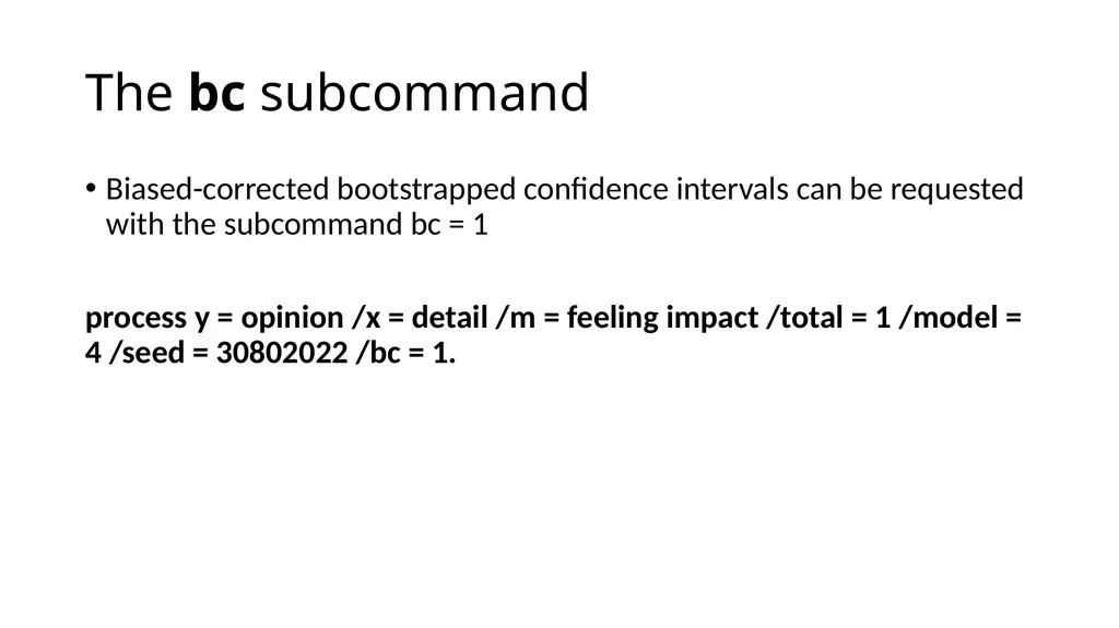
The bc subcommand Biased-corrected bootstrapped confidence intervals can be requested with the subcommand bc = 1
process y = opinion /x = detail /m = feeling impact /total = 1 /model = 4 /seed = 30802022 /bc = 1.<br>
process y = opinion /x = detail /m = feeling impact /total = 1 /model = 4 /seed = 30802022 /bc = 1.<br>
43
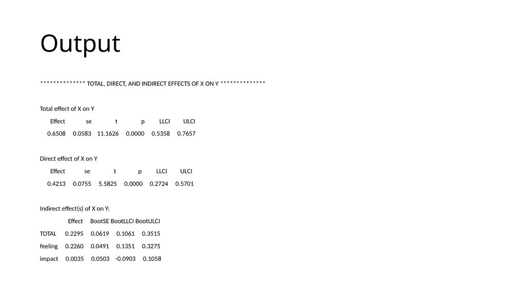
Output ************** TOTAL, DIRECT, AND INDIRECT EFFECTS OF X ON Y **************
Total effect of X on Y
Effect se t p LLCI ULCI
0.6508 0.0583 11.1626 0.0000 0.5358 0.7657
Direct effect of X on Y
Effect se t p LLCI ULCI
0.4213 0.0755 5.5825 0.0000 0.2724 0.5701
Indirect effect(s) of X on Y:
Effect BootSE BootLLCI BootULCI
TOTAL 0.2295 0.0619 0.1061 0.3515
feeling 0.2260 0.0491 0.1351 0.3275
impact 0.0035 0.0503 -0.0903 0.1058<br>
Total effect of X on Y
Effect se t p LLCI ULCI
0.6508 0.0583 11.1626 0.0000 0.5358 0.7657
Direct effect of X on Y
Effect se t p LLCI ULCI
0.4213 0.0755 5.5825 0.0000 0.2724 0.5701
Indirect effect(s) of X on Y:
Effect BootSE BootLLCI BootULCI
TOTAL 0.2295 0.0619 0.1061 0.3515
feeling 0.2260 0.0491 0.1351 0.3275
impact 0.0035 0.0503 -0.0903 0.1058<br>
44
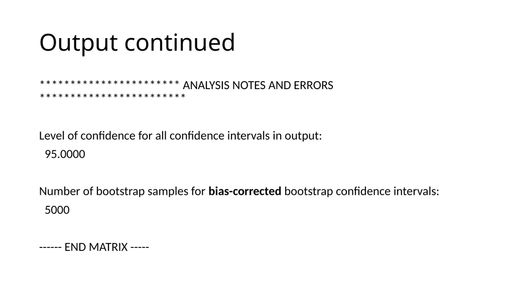
Output continued *********************** ANALYSIS NOTES AND ERRORS ************************
Level of confidence for all confidence intervals in output:
95.0000
Number of bootstrap samples for bias-corrected bootstrap confidence intervals:
5000
------ END MATRIX -----<br>
Level of confidence for all confidence intervals in output:
95.0000
Number of bootstrap samples for bias-corrected bootstrap confidence intervals:
5000
------ END MATRIX -----<br>
45
Question When presenting the results, should you use the original metric of the variables, or should the coefficients be standardized?<br>
46
Answer It depends! (What other answer did you expect??)
If the original metrics of the variables are meaningful, then there may be no need to standardize the results
If the metrics of the variables are arbitrary, then perhaps standardizing is a good idea<br>
If the original metrics of the variables are meaningful, then there may be no need to standardize the results
If the metrics of the variables are arbitrary, then perhaps standardizing is a good idea<br>
47
Hayes’ comments Hayes is careful to note that fully standardized results make sense only when all of the variables in the model are continuous.
He warns against standardizing the coefficients of binary predictors, as this may not make much sense substantively.
If you request standardized coefficients and have specified a binary predictor variable (X), you will get only partially standardized results.
A note to this effect will be given in the final part of the output.<br>
He warns against standardizing the coefficients of binary predictors, as this may not make much sense substantively.
If you request standardized coefficients and have specified a binary predictor variable (X), you will get only partially standardized results.
A note to this effect will be given in the final part of the output.<br>
48
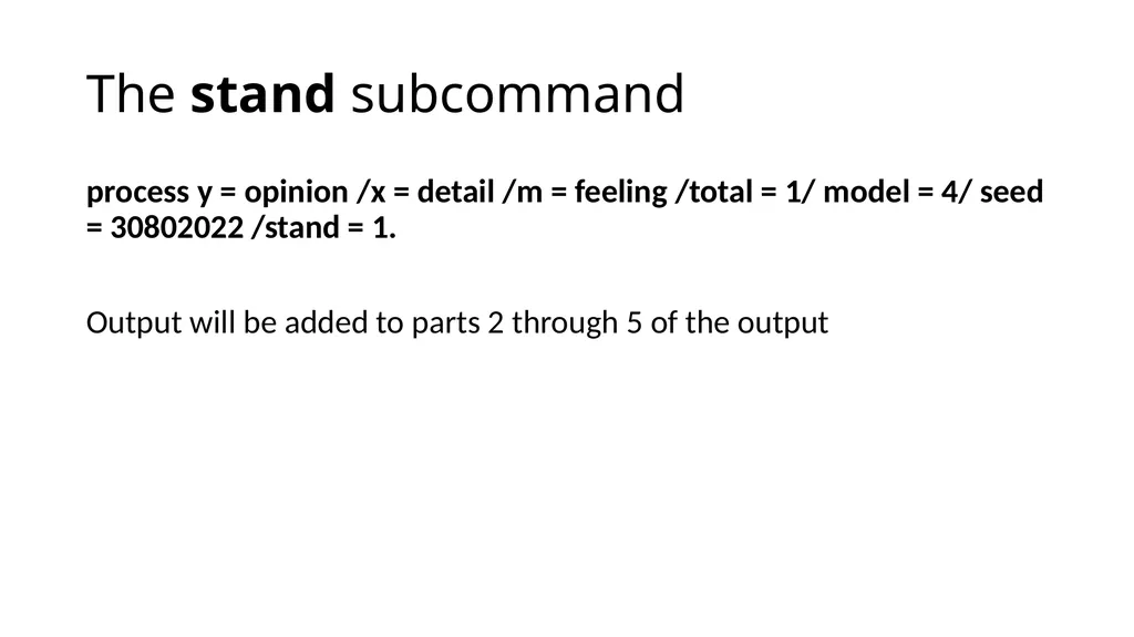
The stand subcommand process y = opinion /x = detail /m = feeling /total = 1/ model = 4/ seed = 30802022 /stand = 1.
Output will be added to parts 2 through 5 of the output<br>
Output will be added to parts 2 through 5 of the output<br>
49
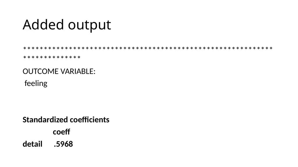
Added output **************************************************************************
OUTCOME VARIABLE:
feeling
Standardized coefficients
coeff
detail .5968<br>
OUTCOME VARIABLE:
feeling
Standardized coefficients
coeff
detail .5968<br>
50
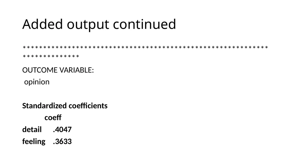
Added output continued **************************************************************************
OUTCOME VARIABLE:
opinion
Standardized coefficients
coeff
detail .4047
feeling .3633<br>
OUTCOME VARIABLE:
opinion
Standardized coefficients
coeff
detail .4047
feeling .3633<br>
51
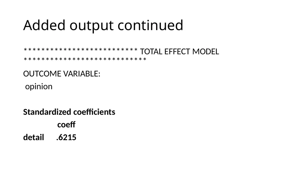
Added output continued ************************** TOTAL EFFECT MODEL ****************************
OUTCOME VARIABLE:
opinion
Standardized coefficients
coeff
detail .6215<br>
OUTCOME VARIABLE:
opinion
Standardized coefficients
coeff
detail .6215<br>
52
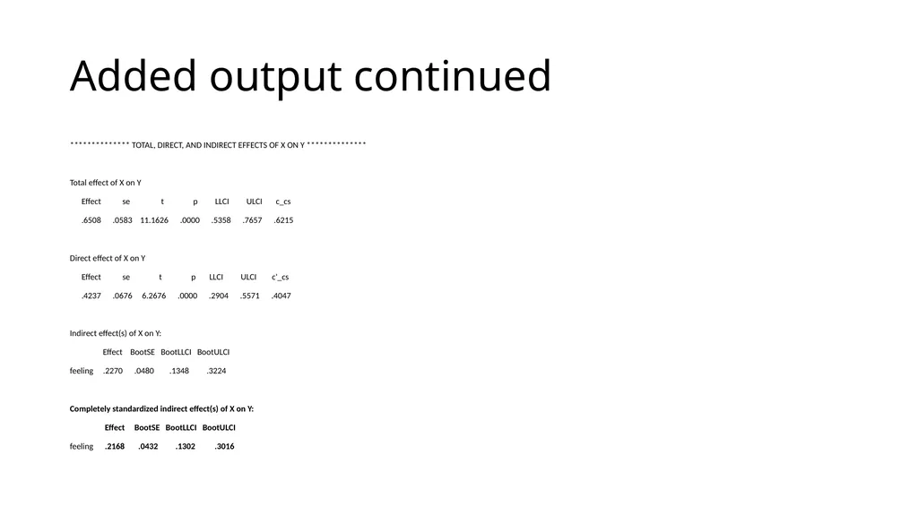
Added output continued ************** TOTAL, DIRECT, AND INDIRECT EFFECTS OF X ON Y **************
Total effect of X on Y
Effect se t p LLCI ULCI c_cs
.6508 .0583 11.1626 .0000 .5358 .7657 .6215
Direct effect of X on Y
Effect se t p LLCI ULCI c'_cs
.4237 .0676 6.2676 .0000 .2904 .5571 .4047
Indirect effect(s) of X on Y:
Effect BootSE BootLLCI BootULCI
feeling .2270 .0480 .1348 .3224
Completely standardized indirect effect(s) of X on Y:
Effect BootSE BootLLCI BootULCI
feeling .2168 .0432 .1302 .3016<br>
Total effect of X on Y
Effect se t p LLCI ULCI c_cs
.6508 .0583 11.1626 .0000 .5358 .7657 .6215
Direct effect of X on Y
Effect se t p LLCI ULCI c'_cs
.4237 .0676 6.2676 .0000 .2904 .5571 .4047
Indirect effect(s) of X on Y:
Effect BootSE BootLLCI BootULCI
feeling .2270 .0480 .1348 .3224
Completely standardized indirect effect(s) of X on Y:
Effect BootSE BootLLCI BootULCI
feeling .2168 .0432 .1302 .3016<br>
53
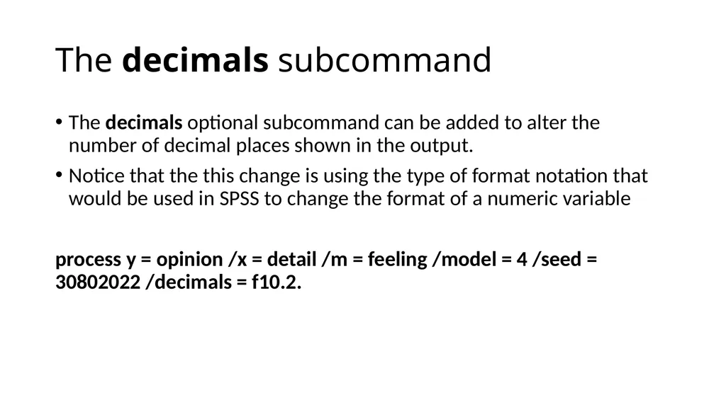
The decimals subcommand The decimals optional subcommand can be added to alter the number of decimal places shown in the output.
Notice that the this change is using the type of format notation that would be used in SPSS to change the format of a numeric variable
process y = opinion /x = detail /m = feeling /model = 4 /seed = 30802022 /decimals = f10.2.<br>
Notice that the this change is using the type of format notation that would be used in SPSS to change the format of a numeric variable
process y = opinion /x = detail /m = feeling /model = 4 /seed = 30802022 /decimals = f10.2.<br>
54
Do you have any questions?<br>
55
Let’s take a short break Let’s come back in five minutes<br>
56
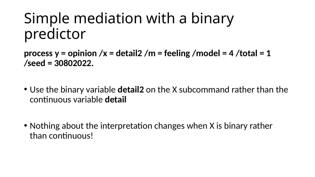
Simple mediation with a binary predictor process y = opinion /x = detail2 /m = feeling /model = 4 /total = 1 /seed = 30802022.
Use the binary variable detail2 on the X subcommand rather than the continuous variable detail
Nothing about the interpretation changes when X is binary rather than continuous!<br>
Use the binary variable detail2 on the X subcommand rather than the continuous variable detail
Nothing about the interpretation changes when X is binary rather than continuous!<br>
57
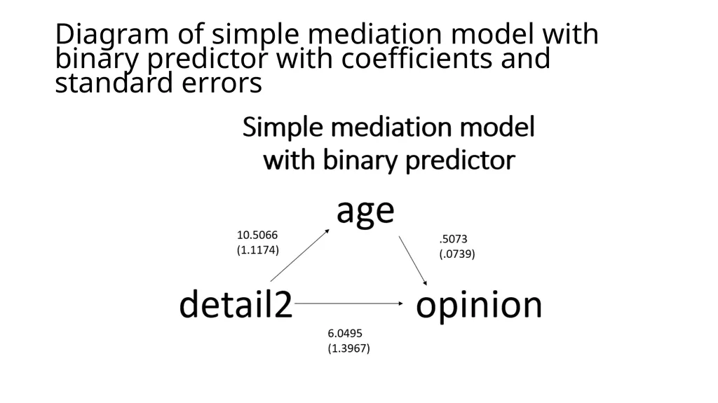
Diagram of simple mediation model with binary predictor with coefficients and standard errors<br>
58
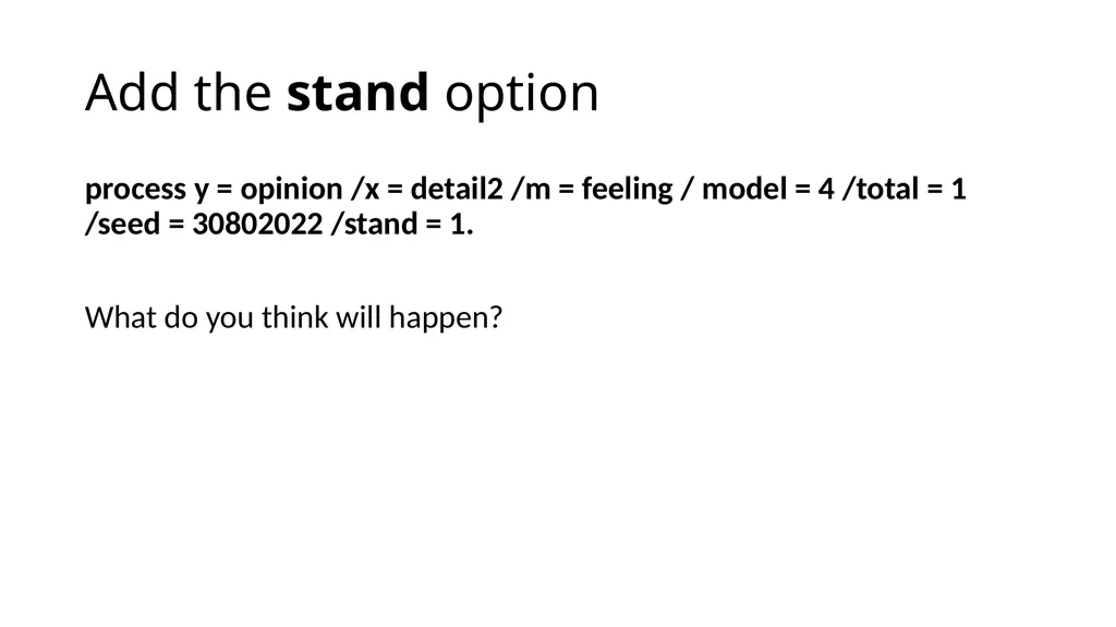
Add the stand option process y = opinion /x = detail2 /m = feeling / model = 4 /total = 1 /seed = 30802022 /stand = 1.
What do you think will happen?<br>
What do you think will happen?<br>
59
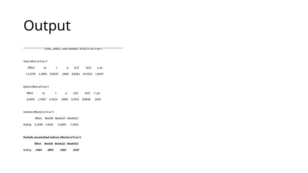
Output ************** TOTAL, DIRECT, AND INDIRECT EFFECTS OF X ON Y **************
Total effect of X on Y
Effect se t p LLCI ULCI c_ps
11.3792 1.2896 8.8239 .0000 8.8361 13.9223 1.0599
Direct effect of X on Y
Effect se t p LLCI ULCI c'_ps
6.0495 1.3967 4.3314 .0000 3.2951 8.8038 .5635
Indirect effect(s) of X on Y:
Effect BootSE BootLLCI BootULCI
feeling 5.3298 1.0324 3.4409 7.4931
Partially standardized indirect effect(s) of X on Y:
Effect BootSE BootLLCI BootULCI
feeling .4964 .0893 .3305 .6767<br>
Total effect of X on Y
Effect se t p LLCI ULCI c_ps
11.3792 1.2896 8.8239 .0000 8.8361 13.9223 1.0599
Direct effect of X on Y
Effect se t p LLCI ULCI c'_ps
6.0495 1.3967 4.3314 .0000 3.2951 8.8038 .5635
Indirect effect(s) of X on Y:
Effect BootSE BootLLCI BootULCI
feeling 5.3298 1.0324 3.4409 7.4931
Partially standardized indirect effect(s) of X on Y:
Effect BootSE BootLLCI BootULCI
feeling .4964 .0893 .3305 .6767<br>
60
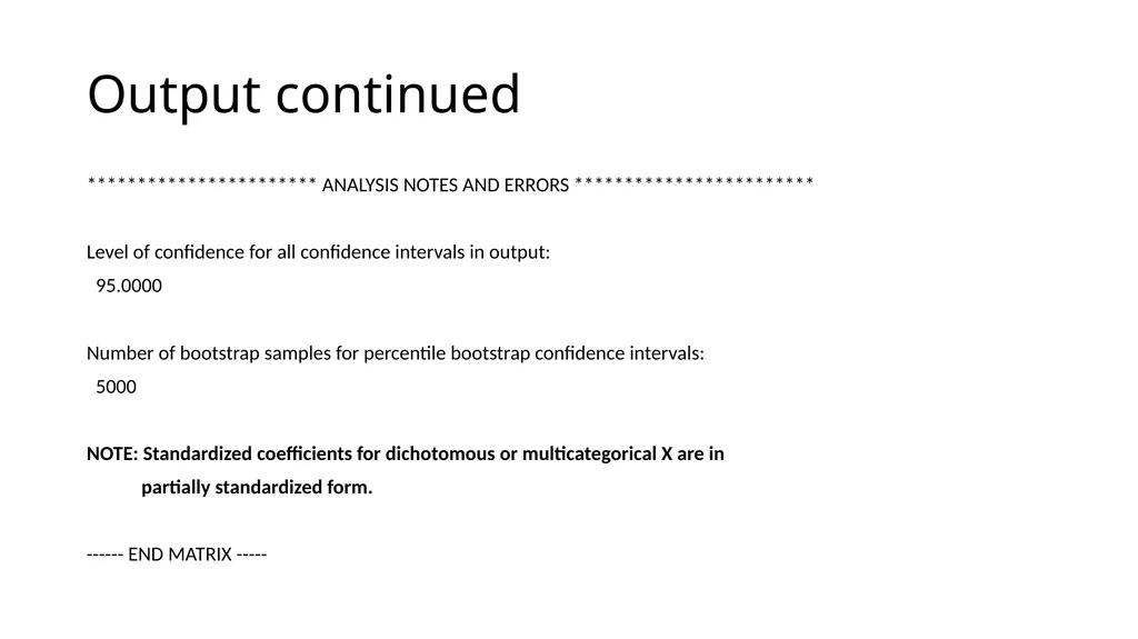
Output continued *********************** ANALYSIS NOTES AND ERRORS ************************
Level of confidence for all confidence intervals in output:
95.0000
Number of bootstrap samples for percentile bootstrap confidence intervals:
5000
NOTE: Standardized coefficients for dichotomous or multicategorical X are in
partially standardized form.
------ END MATRIX -----<br>
Level of confidence for all confidence intervals in output:
95.0000
Number of bootstrap samples for percentile bootstrap confidence intervals:
5000
NOTE: Standardized coefficients for dichotomous or multicategorical X are in
partially standardized form.
------ END MATRIX -----<br>
61
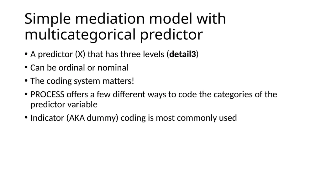
Simple mediation model with multicategorical predictor A predictor (X) that has three levels (detail3)
Can be ordinal or nominal
The coding system matters!
PROCESS offers a few different ways to code the categories of the predictor variable
Indicator (AKA dummy) coding is most commonly used<br>
Can be ordinal or nominal
The coding system matters!
PROCESS offers a few different ways to code the categories of the predictor variable
Indicator (AKA dummy) coding is most commonly used<br>
62
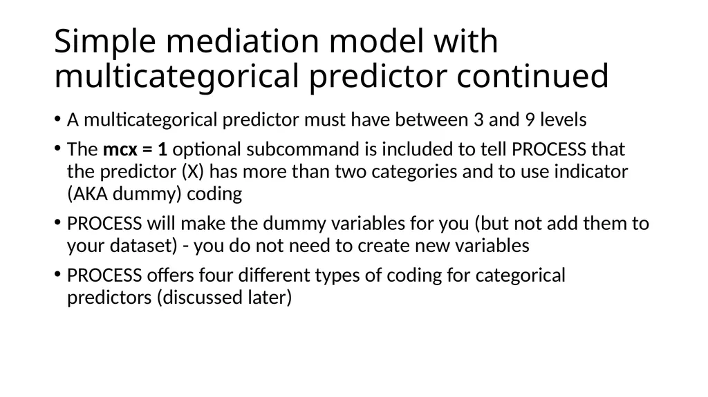
Simple mediation model with multicategorical predictor continued A multicategorical predictor must have between 3 and 9 levels
The mcx = 1 optional subcommand is included to tell PROCESS that the predictor (X) has more than two categories and to use indicator (AKA dummy) coding
PROCESS will make the dummy variables for you (but not add them to your dataset) - you do not need to create new variables
PROCESS offers four different types of coding for categorical predictors (discussed later)<br>
The mcx = 1 optional subcommand is included to tell PROCESS that the predictor (X) has more than two categories and to use indicator (AKA dummy) coding
PROCESS will make the dummy variables for you (but not add them to your dataset) - you do not need to create new variables
PROCESS offers four different types of coding for categorical predictors (discussed later)<br>
63
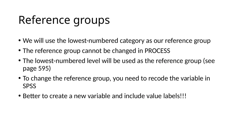
Reference groups We will use the lowest-numbered category as our reference group
The reference group cannot be changed in PROCESS
The lowest-numbered level will be used as the reference group (see page 595)
To change the reference group, you need to recode the variable in SPSS
Better to create a new variable and include value labels!!!<br>
The reference group cannot be changed in PROCESS
The lowest-numbered level will be used as the reference group (see page 595)
To change the reference group, you need to recode the variable in SPSS
Better to create a new variable and include value labels!!!<br>
64
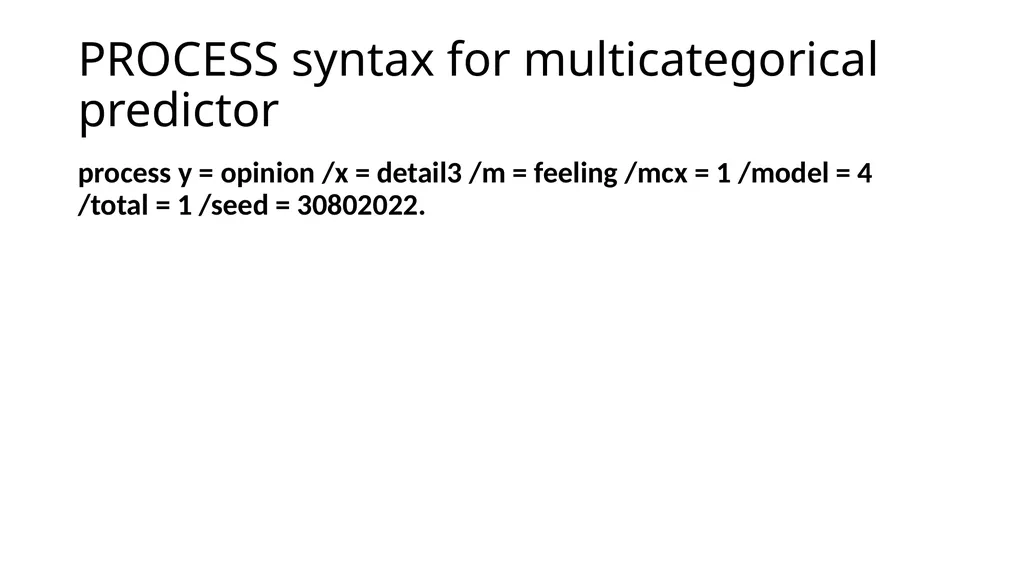
PROCESS syntax for multicategorical predictor process y = opinion /x = detail3 /m = feeling /mcx = 1 /model = 4 /total = 1 /seed = 30802022.<br>
65
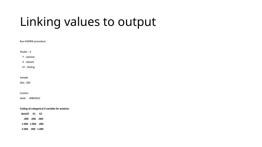
Linking values to output Run MATRIX procedure:
Model : 4
Y : opinion
X : detail3
M : feeling
Sample
Size: 200
Custom
Seed: 30802022
Coding of categorical X variable for analysis:
detail3 X1 X2
.000 .000 .000
1.000 1.000 .000
2.000 .000 1.000<br>
Model : 4
Y : opinion
X : detail3
M : feeling
Sample
Size: 200
Custom
Seed: 30802022
Coding of categorical X variable for analysis:
detail3 X1 X2
.000 .000 .000
1.000 1.000 .000
2.000 .000 1.000<br>
66
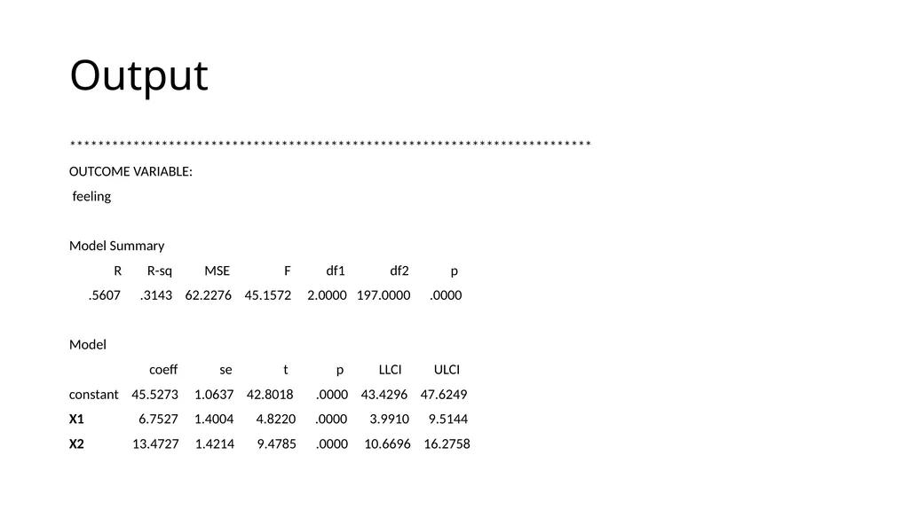
Output **************************************************************************
OUTCOME VARIABLE:
feeling
Model Summary
R R-sq MSE F df1 df2 p
.5607 .3143 62.2276 45.1572 2.0000 197.0000 .0000
Model
coeff se t p LLCI ULCI
constant 45.5273 1.0637 42.8018 .0000 43.4296 47.6249
X1 6.7527 1.4004 4.8220 .0000 3.9910 9.5144
X2 13.4727 1.4214 9.4785 .0000 10.6696 16.2758<br>
OUTCOME VARIABLE:
feeling
Model Summary
R R-sq MSE F df1 df2 p
.5607 .3143 62.2276 45.1572 2.0000 197.0000 .0000
Model
coeff se t p LLCI ULCI
constant 45.5273 1.0637 42.8018 .0000 43.4296 47.6249
X1 6.7527 1.4004 4.8220 .0000 3.9910 9.5144
X2 13.4727 1.4214 9.4785 .0000 10.6696 16.2758<br>
67
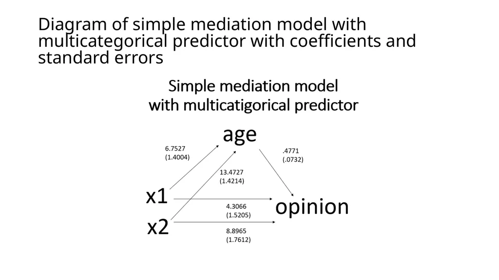
Diagram of simple mediation model with multicategorical predictor with coefficients and standard errors<br>
68
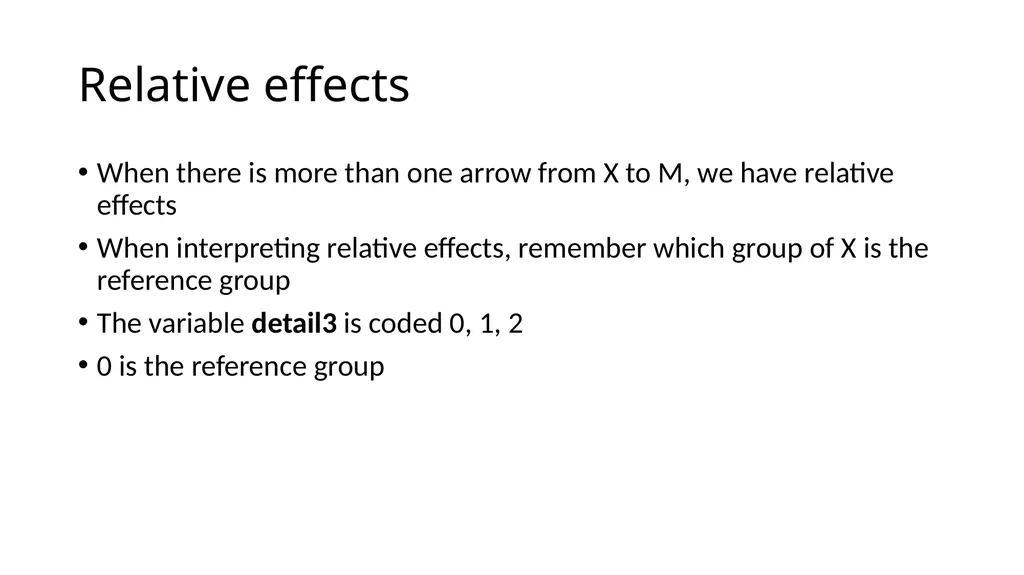
Relative effects When there is more than one arrow from X to M, we have relative effects
When interpreting relative effects, remember which group of X is the reference group
The variable detail3 is coded 0, 1, 2
0 is the reference group<br>
When interpreting relative effects, remember which group of X is the reference group
The variable detail3 is coded 0, 1, 2
0 is the reference group<br>
69
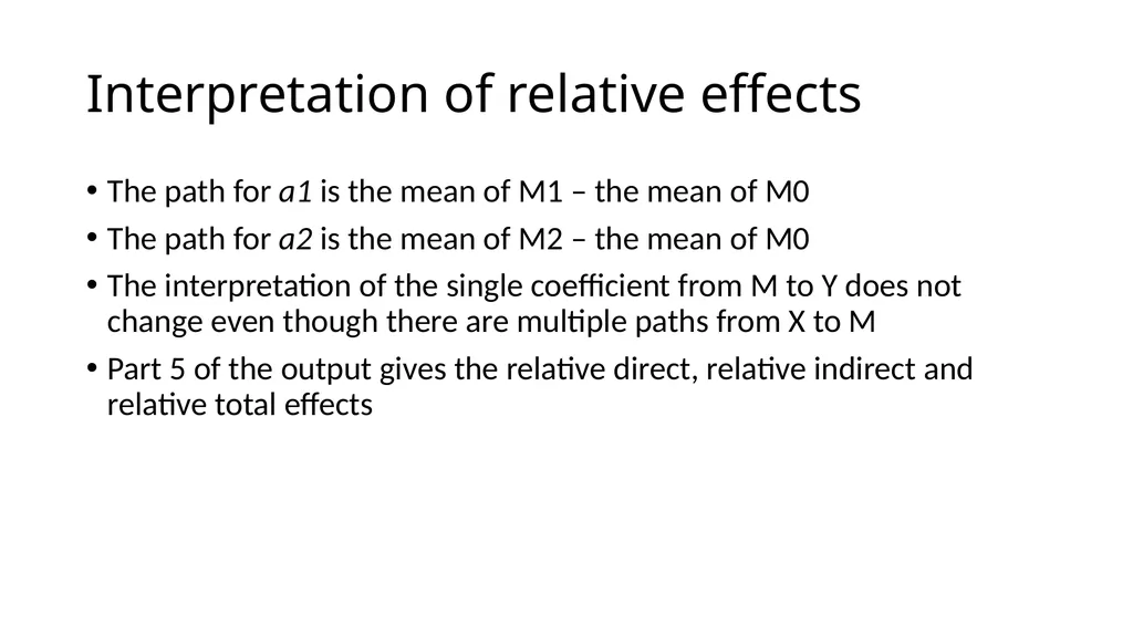
Interpretation of relative effects The path for a1 is the mean of M1 – the mean of M0
The path for a2 is the mean of M2 – the mean of M0
The interpretation of the single coefficient from M to Y does not change even though there are multiple paths from X to M
Part 5 of the output gives the relative direct, relative indirect and relative total effects<br>
The path for a2 is the mean of M2 – the mean of M0
The interpretation of the single coefficient from M to Y does not change even though there are multiple paths from X to M
Part 5 of the output gives the relative direct, relative indirect and relative total effects<br>
70
Can you calculate the relative indirect and relative total effects by hand? Let’s take a minute to try this!<br>
71
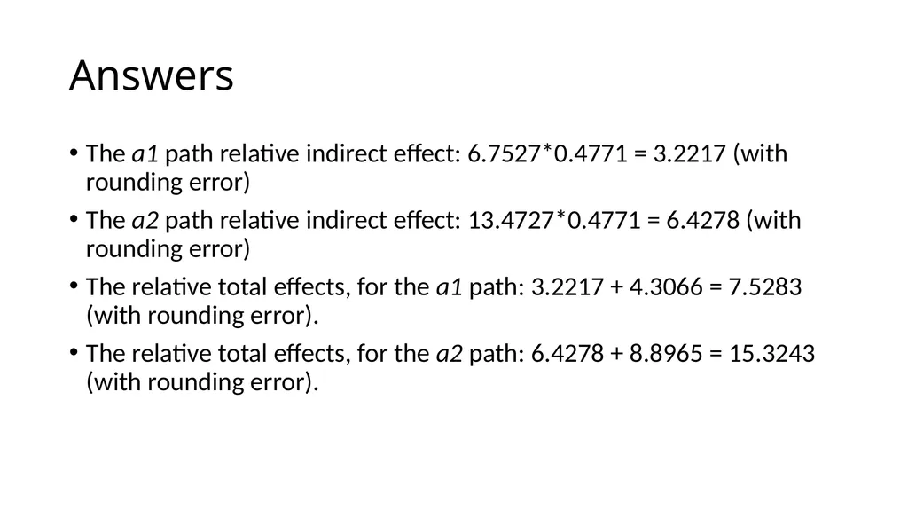
Answers The a1 path relative indirect effect: 6.7527*0.4771 = 3.2217 (with rounding error)
The a2 path relative indirect effect: 13.4727*0.4771 = 6.4278 (with rounding error)
The relative total effects, for the a1 path: 3.2217 + 4.3066 = 7.5283 (with rounding error).
The relative total effects, for the a2 path: 6.4278 + 8.8965 = 15.3243 (with rounding error).<br>
The a2 path relative indirect effect: 13.4727*0.4771 = 6.4278 (with rounding error)
The relative total effects, for the a1 path: 3.2217 + 4.3066 = 7.5283 (with rounding error).
The relative total effects, for the a2 path: 6.4278 + 8.8965 = 15.3243 (with rounding error).<br>
72
Omnibus tests Omnibus (AKA multi-degree-of-freedom) tests of these effects are also provided in the output
These omnibus tests are used to determine if the overall effect is statistically significant
The omnibus tests should be included in the reporting of the results<br>
These omnibus tests are used to determine if the overall effect is statistically significant
The omnibus tests should be included in the reporting of the results<br>
73
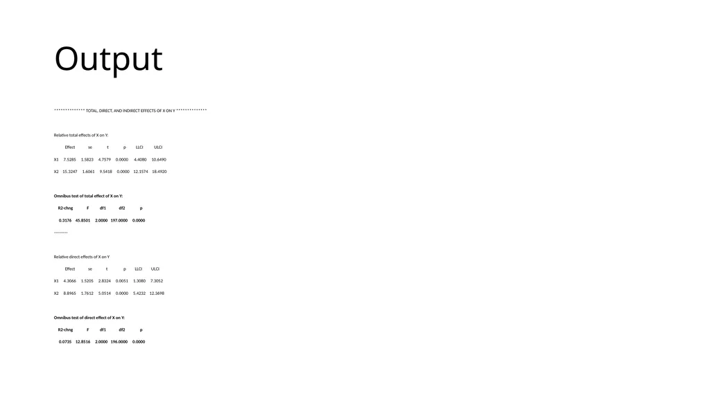
Output ************** TOTAL, DIRECT, AND INDIRECT EFFECTS OF X ON Y **************
Relative total effects of X on Y:
Effect se t p LLCI ULCI
X1 7.5285 1.5823 4.7579 0.0000 4.4080 10.6490
X2 15.3247 1.6061 9.5418 0.0000 12.1574 18.4920
Omnibus test of total effect of X on Y:
R2-chng F df1 df2 p
0.3176 45.8501 2.0000 197.0000 0.0000
----------
Relative direct effects of X on Y
Effect se t p LLCI ULCI
X1 4.3066 1.5205 2.8324 0.0051 1.3080 7.3052
X2 8.8965 1.7612 5.0514 0.0000 5.4232 12.3698
Omnibus test of direct effect of X on Y:
R2-chng F df1 df2 p
0.0735 12.8516 2.0000 196.0000 0.0000<br>
Relative total effects of X on Y:
Effect se t p LLCI ULCI
X1 7.5285 1.5823 4.7579 0.0000 4.4080 10.6490
X2 15.3247 1.6061 9.5418 0.0000 12.1574 18.4920
Omnibus test of total effect of X on Y:
R2-chng F df1 df2 p
0.3176 45.8501 2.0000 197.0000 0.0000
----------
Relative direct effects of X on Y
Effect se t p LLCI ULCI
X1 4.3066 1.5205 2.8324 0.0051 1.3080 7.3052
X2 8.8965 1.7612 5.0514 0.0000 5.4232 12.3698
Omnibus test of direct effect of X on Y:
R2-chng F df1 df2 p
0.0735 12.8516 2.0000 196.0000 0.0000<br>
74
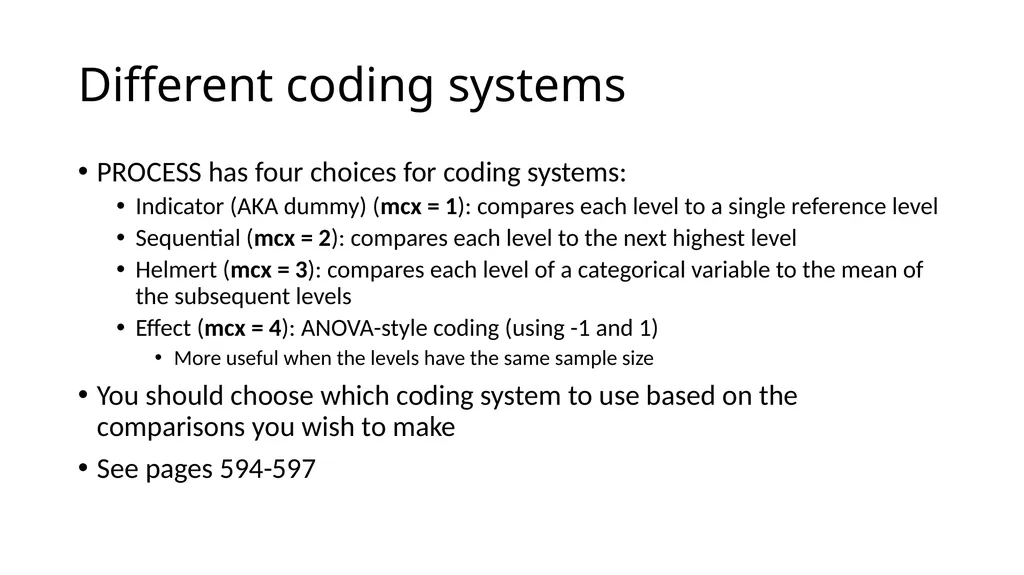
Different coding systems PROCESS has four choices for coding systems:
Indicator (AKA dummy) (mcx = 1): compares each level to a single reference level
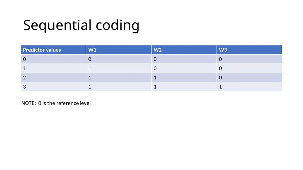
Sequential (mcx = 2): compares each level to the next highest level
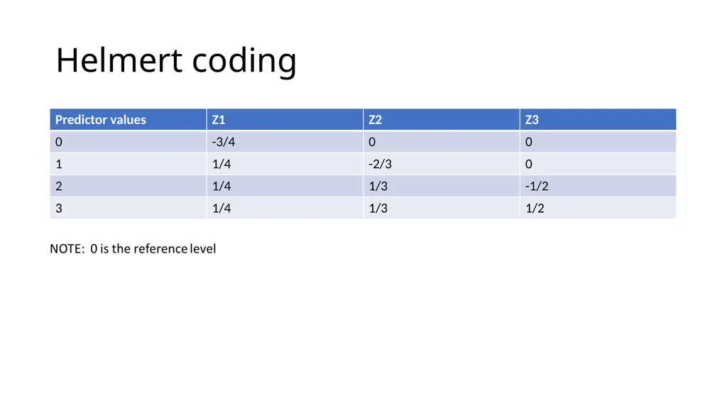
Helmert (mcx = 3): compares each level of a categorical variable to the mean of the subsequent levels
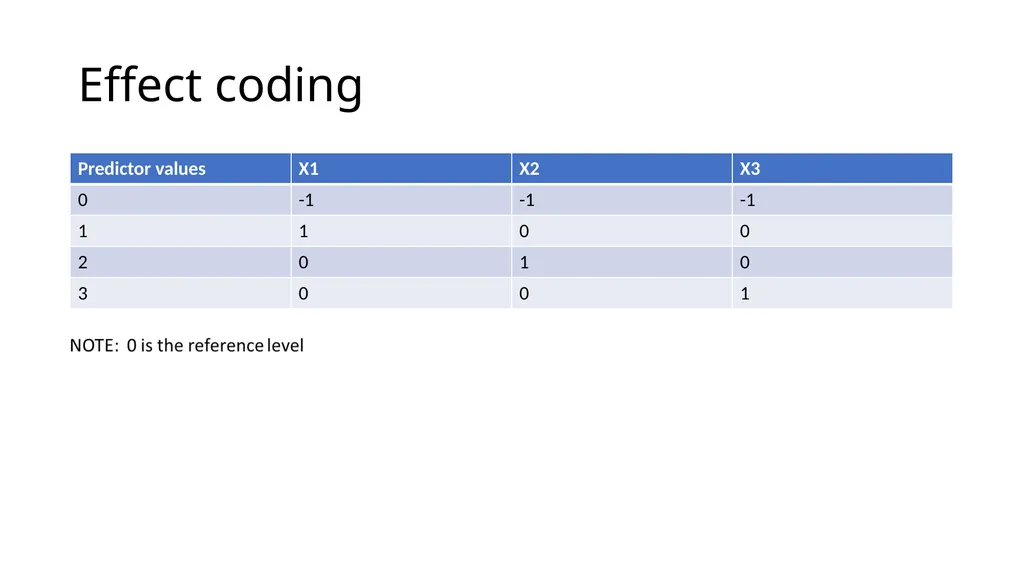
Effect (mcx = 4): ANOVA-style coding (using -1 and 1)
More useful when the levels have the same sample size
You should choose which coding system to use based on the comparisons you wish to make
See pages 594-597<br>
Indicator (AKA dummy) (mcx = 1): compares each level to a single reference level
Sequential (mcx = 2): compares each level to the next highest level
Helmert (mcx = 3): compares each level of a categorical variable to the mean of the subsequent levels
Effect (mcx = 4): ANOVA-style coding (using -1 and 1)
More useful when the levels have the same sample size
You should choose which coding system to use based on the comparisons you wish to make
See pages 594-597<br>
75
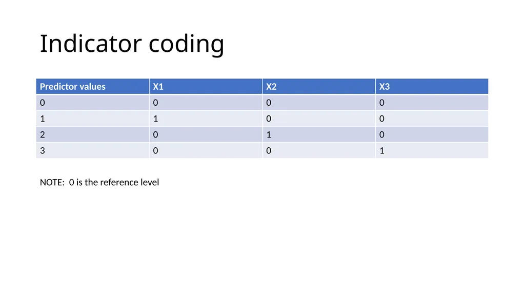
Indicator coding NOTE: 0 is the reference level<br>
76
Sequential coding<br>
77
Helmert coding<br>
78
Effect coding<br>
79
Custom coding You can also use your own coding system
See pages 596-597 for an example<br>
See pages 596-597 for an example<br>
80
Omnibus tests, AKA multi-degree-of-freedom tests The omnibus test will be the same regardless of which coding system you use
The values of the coefficients will be different, and the associated p-values may be different as well
A coefficient may be statistically significant using one coding system and not statistically significant using a different coding system<br>
The values of the coefficients will be different, and the associated p-values may be different as well
A coefficient may be statistically significant using one coding system and not statistically significant using a different coding system<br>
81
Do you have any questions?<br>
82
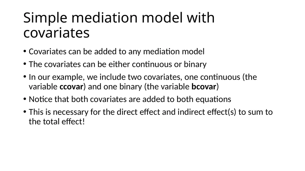
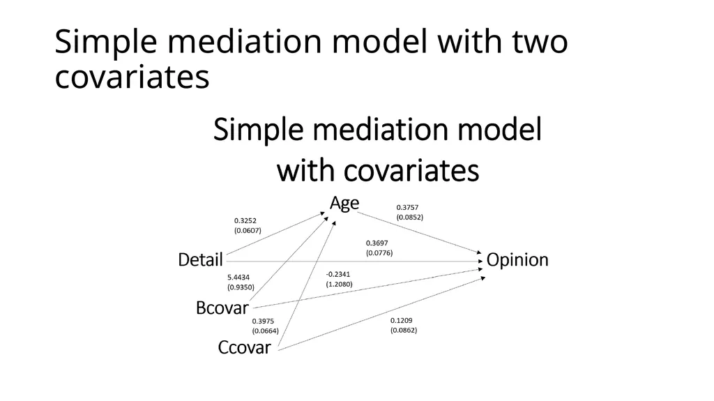
Simple mediation model with covariates Covariates can be added to any mediation model
The covariates can be either continuous or binary
In our example, we include two covariates, one continuous (the variable ccovar) and one binary (the variable bcovar)
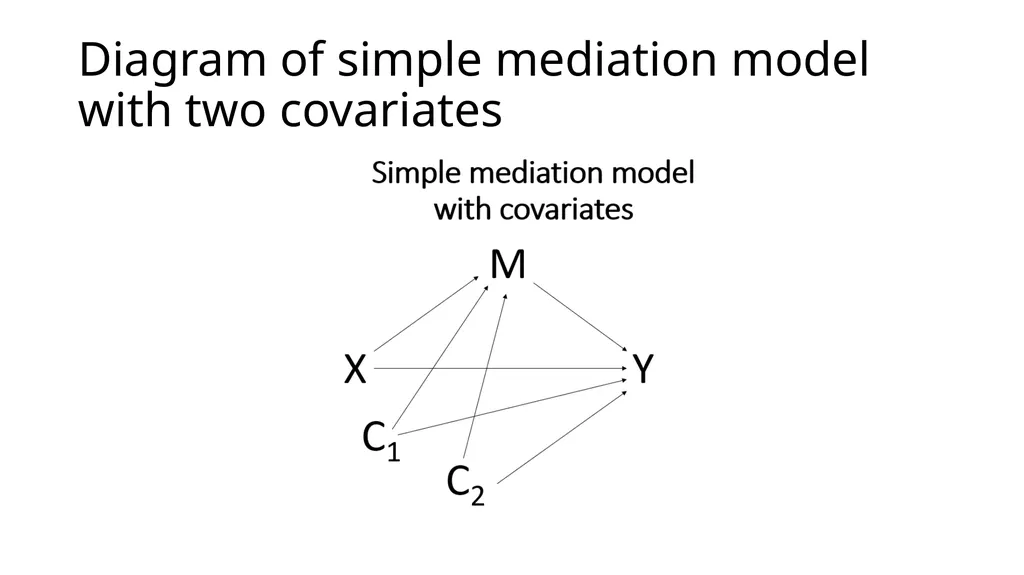
Notice that both covariates are added to both equations
This is necessary for the direct effect and indirect effect(s) to sum to the total effect!<br>
The covariates can be either continuous or binary
In our example, we include two covariates, one continuous (the variable ccovar) and one binary (the variable bcovar)
Notice that both covariates are added to both equations
This is necessary for the direct effect and indirect effect(s) to sum to the total effect!<br>
83
Diagram of simple mediation model with two covariates<br>
84
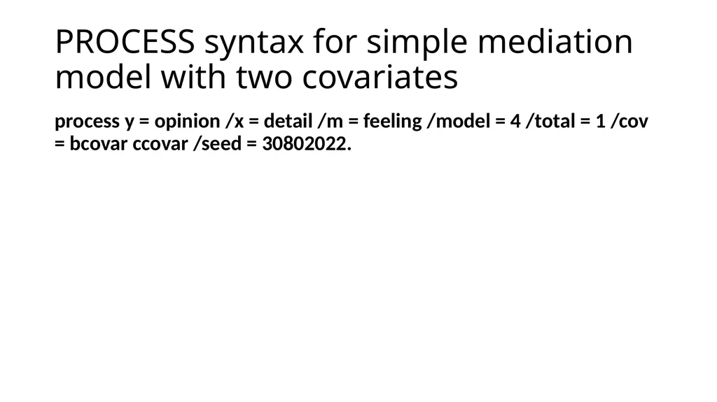
PROCESS syntax for simple mediation model with two covariates process y = opinion /x = detail /m = feeling /model = 4 /total = 1 /cov = bcovar ccovar /seed = 30802022.<br>
85
The output Information about the covariates is included at the bottom of parts 2 through 4 of the output
The interpretation of the path coefficients is just the same as before, except that we now add "holding the covariates constant" to the discussion of the path coefficients<br>
The interpretation of the path coefficients is just the same as before, except that we now add "holding the covariates constant" to the discussion of the path coefficients<br>
86
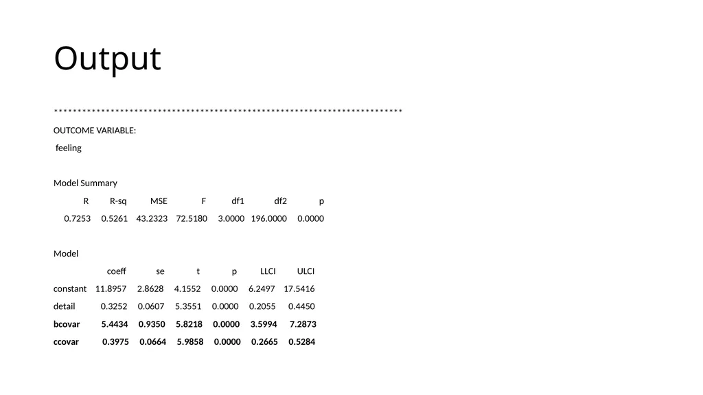
Output **************************************************************************
OUTCOME VARIABLE:
feeling
Model Summary
R R-sq MSE F df1 df2 p
0.7253 0.5261 43.2323 72.5180 3.0000 196.0000 0.0000
Model
coeff se t p LLCI ULCI
constant 11.8957 2.8628 4.1552 0.0000 6.2497 17.5416
detail 0.3252 0.0607 5.3551 0.0000 0.2055 0.4450
bcovar 5.4434 0.9350 5.8218 0.0000 3.5994 7.2873
ccovar 0.3975 0.0664 5.9858 0.0000 0.2665 0.5284<br>
OUTCOME VARIABLE:
feeling
Model Summary
R R-sq MSE F df1 df2 p
0.7253 0.5261 43.2323 72.5180 3.0000 196.0000 0.0000
Model
coeff se t p LLCI ULCI
constant 11.8957 2.8628 4.1552 0.0000 6.2497 17.5416
detail 0.3252 0.0607 5.3551 0.0000 0.2055 0.4450
bcovar 5.4434 0.9350 5.8218 0.0000 3.5994 7.2873
ccovar 0.3975 0.0664 5.9858 0.0000 0.2665 0.5284<br>
87
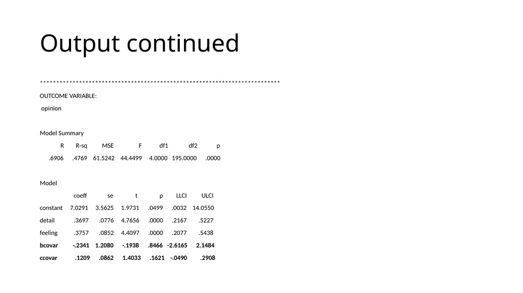
Output continued **************************************************************************
OUTCOME VARIABLE:
opinion
Model Summary
R R-sq MSE F df1 df2 p
.6906 .4769 61.5242 44.4499 4.0000 195.0000 .0000
Model
coeff se t p LLCI ULCI
constant 7.0291 3.5625 1.9731 .0499 .0032 14.0550
detail .3697 .0776 4.7656 .0000 .2167 .5227
feeling .3757 .0852 4.4097 .0000 .2077 .5438
bcovar -.2341 1.2080 -.1938 .8466 -2.6165 2.1484
ccovar .1209 .0862 1.4033 .1621 -.0490 .2908<br>
OUTCOME VARIABLE:
opinion
Model Summary
R R-sq MSE F df1 df2 p
.6906 .4769 61.5242 44.4499 4.0000 195.0000 .0000
Model
coeff se t p LLCI ULCI
constant 7.0291 3.5625 1.9731 .0499 .0032 14.0550
detail .3697 .0776 4.7656 .0000 .2167 .5227
feeling .3757 .0852 4.4097 .0000 .2077 .5438
bcovar -.2341 1.2080 -.1938 .8466 -2.6165 2.1484
ccovar .1209 .0862 1.4033 .1621 -.0490 .2908<br>
88
Simple mediation model with two covariates<br>
89
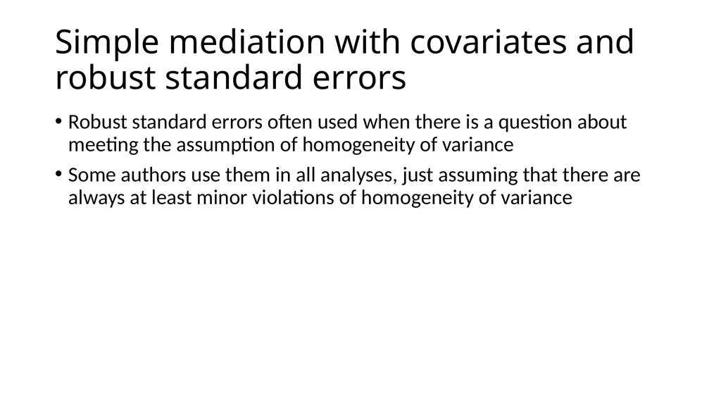
Simple mediation with covariates and robust standard errors Robust standard errors often used when there is a question about meeting the assumption of homogeneity of variance
Some authors use them in all analyses, just assuming that there are always at least minor violations of homogeneity of variance<br>
Some authors use them in all analyses, just assuming that there are always at least minor violations of homogeneity of variance<br>
90
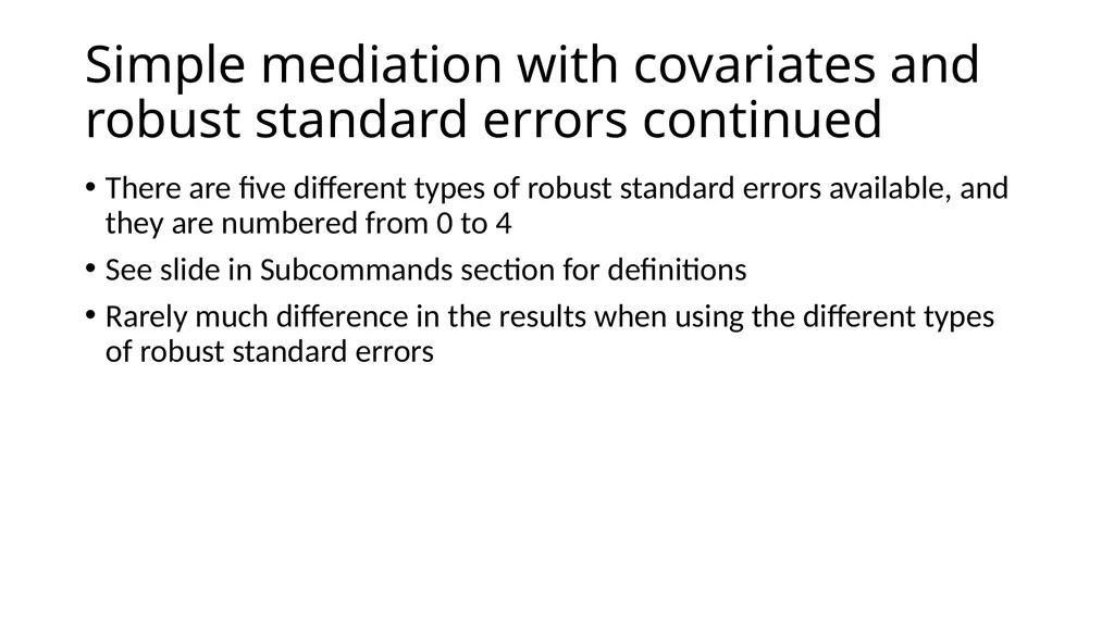
Simple mediation with covariates and robust standard errors continued There are five different types of robust standard errors available, and they are numbered from 0 to 4
See slide in Subcommands section for definitions
Rarely much difference in the results when using the different types of robust standard errors<br>
See slide in Subcommands section for definitions
Rarely much difference in the results when using the different types of robust standard errors<br>
91
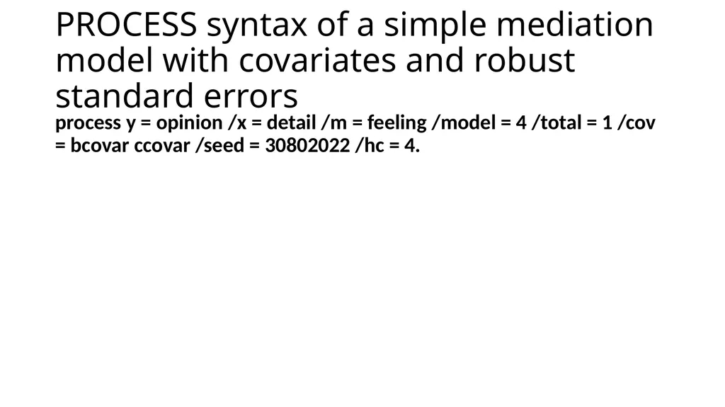
PROCESS syntax of a simple mediation model with covariates and robust standard errors process y = opinion /x = detail /m = feeling /model = 4 /total = 1 /cov = bcovar ccovar /seed = 30802022 /hc = 4.<br>
92
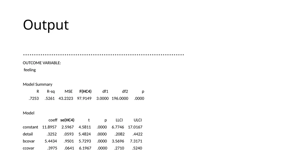
Output **************************************************************************
OUTCOME VARIABLE:
feeling
Model Summary
R R-sq MSE F(HC4) df1 df2 p
.7253 .5261 43.2323 97.9149 3.0000 196.0000 .0000
Model
coeff se(HC4) t p LLCI ULCI
constant 11.8957 2.5967 4.5811 .0000 6.7746 17.0167
detail .3252 .0593 5.4824 .0000 .2082 .4422
bcovar 5.4434 .9501 5.7293 .0000 3.5696 7.3171
ccovar .3975 .0641 6.1967 .0000 .2710 .5240<br>
OUTCOME VARIABLE:
feeling
Model Summary
R R-sq MSE F(HC4) df1 df2 p
.7253 .5261 43.2323 97.9149 3.0000 196.0000 .0000
Model
coeff se(HC4) t p LLCI ULCI
constant 11.8957 2.5967 4.5811 .0000 6.7746 17.0167
detail .3252 .0593 5.4824 .0000 .2082 .4422
bcovar 5.4434 .9501 5.7293 .0000 3.5696 7.3171
ccovar .3975 .0641 6.1967 .0000 .2710 .5240<br>
93
Output continued **************************************************************************
OUTCOME VARIABLE:
opinion
Model Summary
R R-sq MSE F(HC4) df1 df2 p
.6906 .4769 61.5242 53.9715 4.0000 195.0000 .0000
Model
coeff se(HC4) t p LLCI ULCI
constant 7.0291 3.4393 2.0437 .0423 .2460 13.8122
detail .3697 .0761 4.8583 .0000 .2196 .5198
feeling .3757 .0909 4.1347 .0001 .1965 .5550
bcovar -.2341 1.1511 -.2033 .8391 -2.5043 2.0362
ccovar .1209 .0926 1.3052 .1934 -.0618 .3036<br>
OUTCOME VARIABLE:
opinion
Model Summary
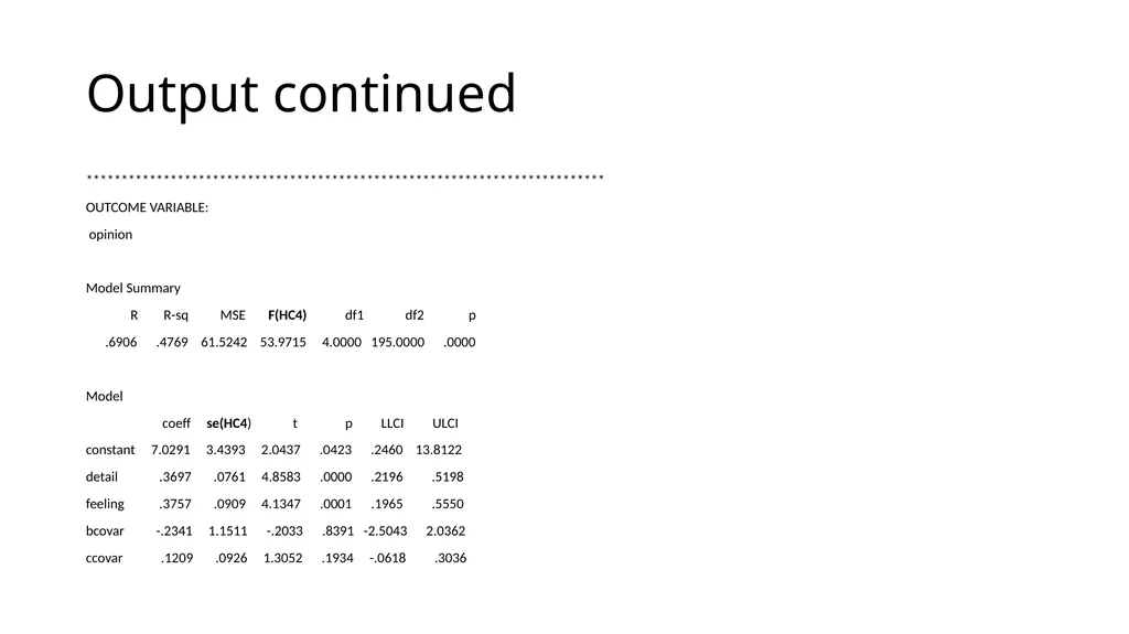
R R-sq MSE F(HC4) df1 df2 p
.6906 .4769 61.5242 53.9715 4.0000 195.0000 .0000
Model
coeff se(HC4) t p LLCI ULCI
constant 7.0291 3.4393 2.0437 .0423 .2460 13.8122
detail .3697 .0761 4.8583 .0000 .2196 .5198
feeling .3757 .0909 4.1347 .0001 .1965 .5550
bcovar -.2341 1.1511 -.2033 .8391 -2.5043 2.0362
ccovar .1209 .0926 1.3052 .1934 -.0618 .3036<br>
94
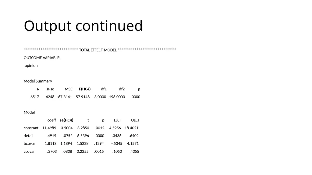
Output continued ************************** TOTAL EFFECT MODEL ****************************
OUTCOME VARIABLE:
opinion
Model Summary
R R-sq MSE F(HC4) df1 df2 p
.6517 .4248 67.3141 57.9148 3.0000 196.0000 .0000
Model
coeff se(HC4) t p LLCI ULCI
constant 11.4989 3.5004 3.2850 .0012 4.5956 18.4021
detail .4919 .0752 6.5396 .0000 .3436 .6402
bcovar 1.8113 1.1894 1.5228 .1294 -.5345 4.1571
ccovar .2703 .0838 3.2255 .0015 .1050 .4355<br>
OUTCOME VARIABLE:
opinion
Model Summary
R R-sq MSE F(HC4) df1 df2 p
.6517 .4248 67.3141 57.9148 3.0000 196.0000 .0000
Model
coeff se(HC4) t p LLCI ULCI
constant 11.4989 3.5004 3.2850 .0012 4.5956 18.4021
detail .4919 .0752 6.5396 .0000 .3436 .6402
bcovar 1.8113 1.1894 1.5228 .1294 -.5345 4.1571
ccovar .2703 .0838 3.2255 .0015 .1050 .4355<br>
95
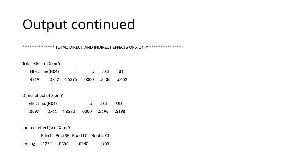
Output continued ************** TOTAL, DIRECT, AND INDIRECT EFFECTS OF X ON Y **************
Total effect of X on Y
Effect se(HC4) t p LLCI ULCI
.4919 .0752 6.5396 .0000 .3436 .6402
Direct effect of X on Y
Effect se(HC4) t p LLCI ULCI
.3697 .0761 4.8583 .0000 .2196 .5198
Indirect effect(s) of X on Y:
Effect BootSE BootLLCI BootULCI
feeling .1222 .0356 .0580 .1965<br>
Total effect of X on Y
Effect se(HC4) t p LLCI ULCI
.4919 .0752 6.5396 .0000 .3436 .6402
Direct effect of X on Y
Effect se(HC4) t p LLCI ULCI
.3697 .0761 4.8583 .0000 .2196 .5198
Indirect effect(s) of X on Y:
Effect BootSE BootLLCI BootULCI
feeling .1222 .0356 .0580 .1965<br>
96
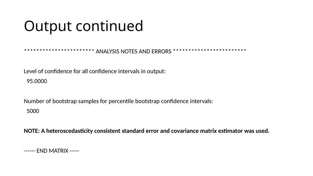
Output continued *********************** ANALYSIS NOTES AND ERRORS ************************
Level of confidence for all confidence intervals in output:
95.0000
Number of bootstrap samples for percentile bootstrap confidence intervals:
5000
NOTE: A heteroscedasticity consistent standard error and covariance matrix estimator was used.
------ END MATRIX -----<br>
Level of confidence for all confidence intervals in output:
95.0000
Number of bootstrap samples for percentile bootstrap confidence intervals:
5000
NOTE: A heteroscedasticity consistent standard error and covariance matrix estimator was used.
------ END MATRIX -----<br>
97
Multiple predictor variabls The PROCESS macro only allows for a single predictor variable
If you want to have two or more predictor variables in your mediation model, you can “trick” PROCESS into including the additional predictor variables as covariates
Remember that predictors and covariates are the same thing (i.e., independent variables) in regression models<br>
If you want to have two or more predictor variables in your mediation model, you can “trick” PROCESS into including the additional predictor variables as covariates
Remember that predictors and covariates are the same thing (i.e., independent variables) in regression models<br>
98
Question Should you run separate models for each predictor, or should you run a single model that includes all of the predictors?<br>
99
Answer It depends!
Depends on each individual research situation
The research question to be addressed, the sample size, the number of tests that will results from each option (keeping an eye on the alpha inflation problem), etc.<br>
Depends on each individual research situation
The research question to be addressed, the sample size, the number of tests that will results from each option (keeping an eye on the alpha inflation problem), etc.<br>
100
Do you have any questions?<br>
101
Let’s take a short break!<br>
102
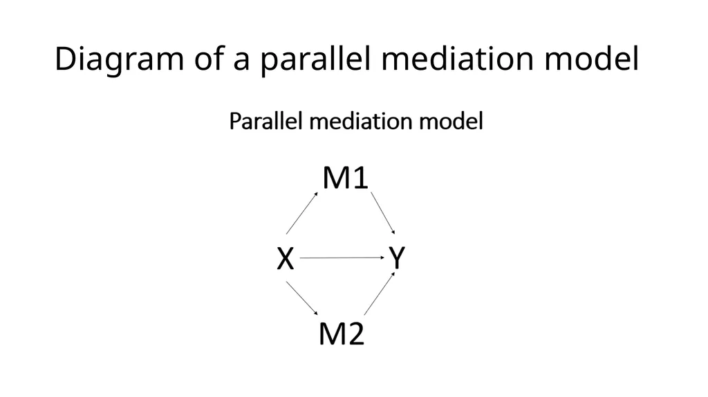
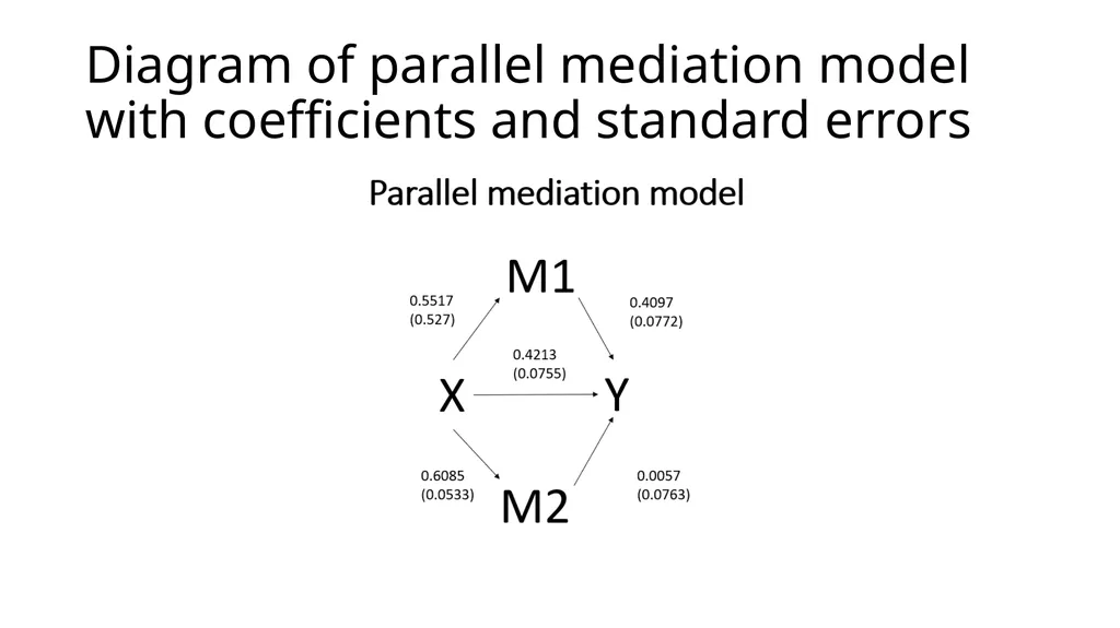
Parallel mediation Two (or more) mediators, both of which are between the predictor and outcome
Have two sets of indirect effects: the indirect effect going through the first mediator, and the indirect effect going through the second mediator
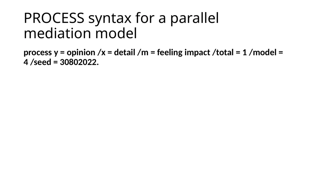
In PROCESS, you simply add list all of the mediators in any order on the m subcommand and use model 4<br>
Have two sets of indirect effects: the indirect effect going through the first mediator, and the indirect effect going through the second mediator
In PROCESS, you simply add list all of the mediators in any order on the m subcommand and use model 4<br>
103
Diagram of a parallel mediation model<br>
104
PROCESS syntax for a parallel mediation model process y = opinion /x = detail /m = feeling impact /total = 1 /model = 4 /seed = 30802022.<br>
105
Diagram of parallel mediation model with coefficients and standard errors<br>
106
Do you have any questions?<br>
107
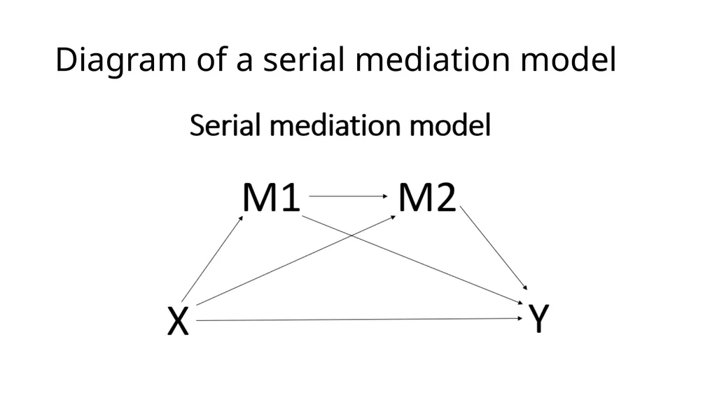
Serail mediation The mediators are ordered between the predictor and the outcome
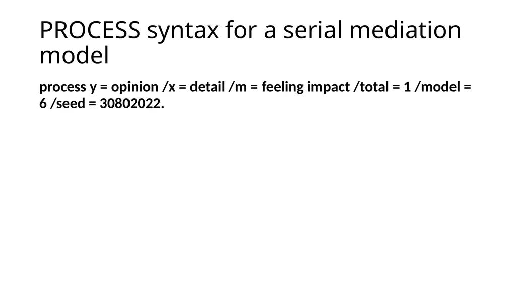
When specifying a serial mediation model, the order in which the mediators are listed on the m subcommand is important!
The first mediator that you list is the first mediator in the model, the second mediator that you list is the second one in the model, and so on
PROCESS will allow up to six mediators in a single model, although there are few research situations (or datasets) that would allow for so many mediators<br>
When specifying a serial mediation model, the order in which the mediators are listed on the m subcommand is important!
The first mediator that you list is the first mediator in the model, the second mediator that you list is the second one in the model, and so on
PROCESS will allow up to six mediators in a single model, although there are few research situations (or datasets) that would allow for so many mediators<br>
108
Diagram of a serial mediation model<br>
109
PROCESS syntax for a serial mediation model process y = opinion /x = detail /m = feeling impact /total = 1 /model = 6 /seed = 30802022.<br>
110
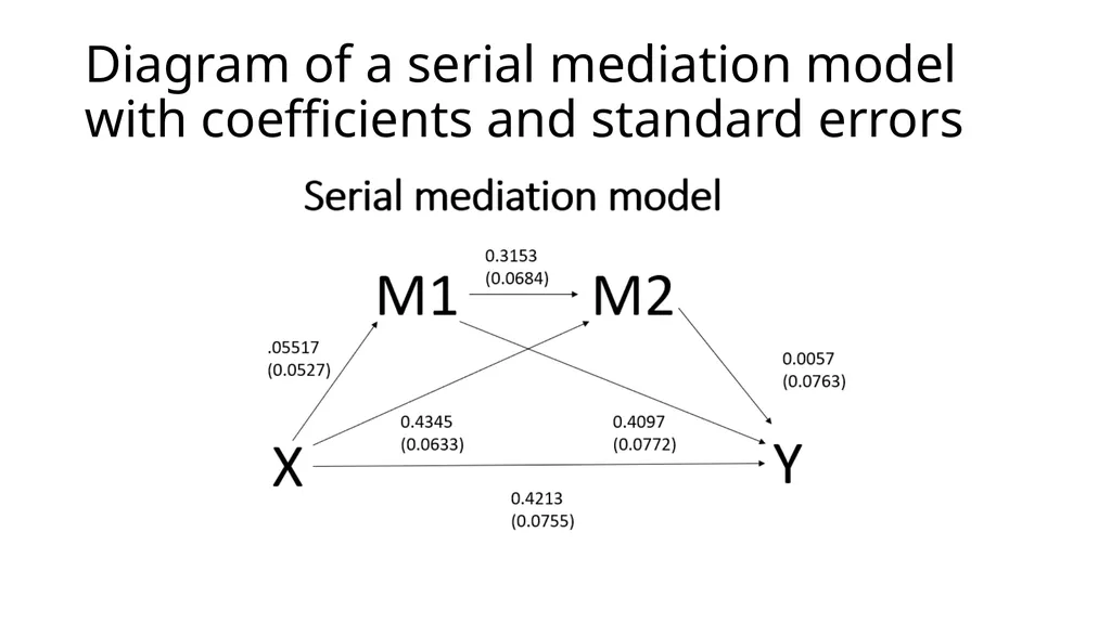
Diagram of a serial mediation model with coefficients and standard errors<br>
111
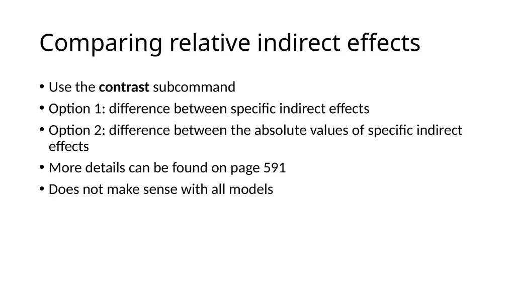
Comparing relative indirect effects Use the contrast subcommand
Option 1: difference between specific indirect effects
Option 2: difference between the absolute values of specific indirect effects
More details can be found on page 591
Does not make sense with all models<br>
Option 1: difference between specific indirect effects
Option 2: difference between the absolute values of specific indirect effects
More details can be found on page 591
Does not make sense with all models<br>
112
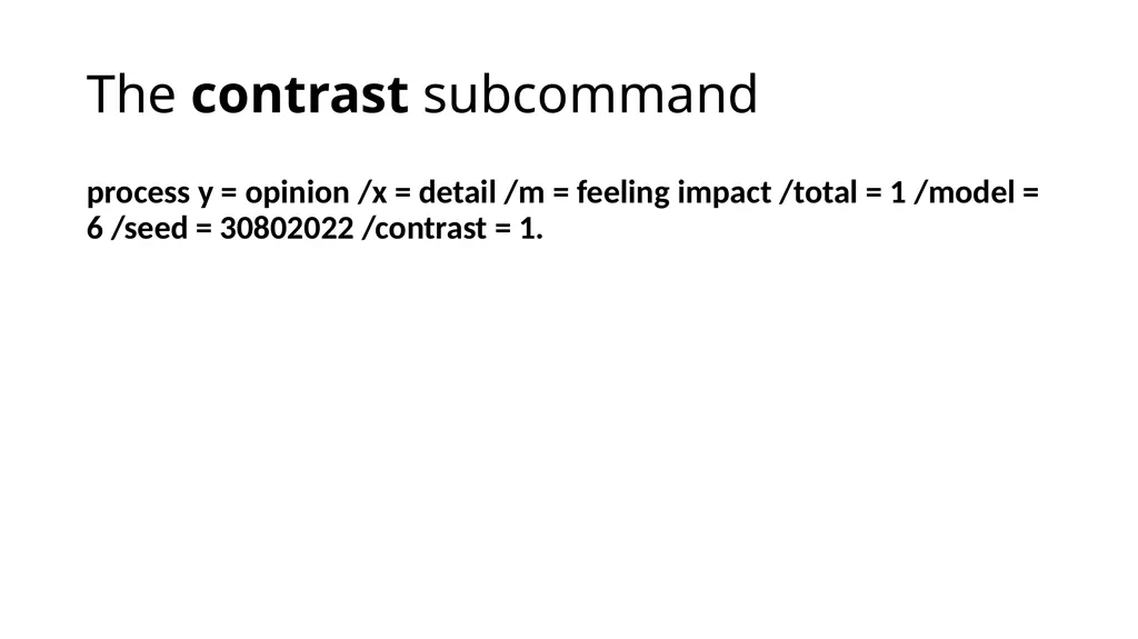
The contrast subcommand process y = opinion /x = detail /m = feeling impact /total = 1 /model = 6 /seed = 30802022 /contrast = 1.<br>
113
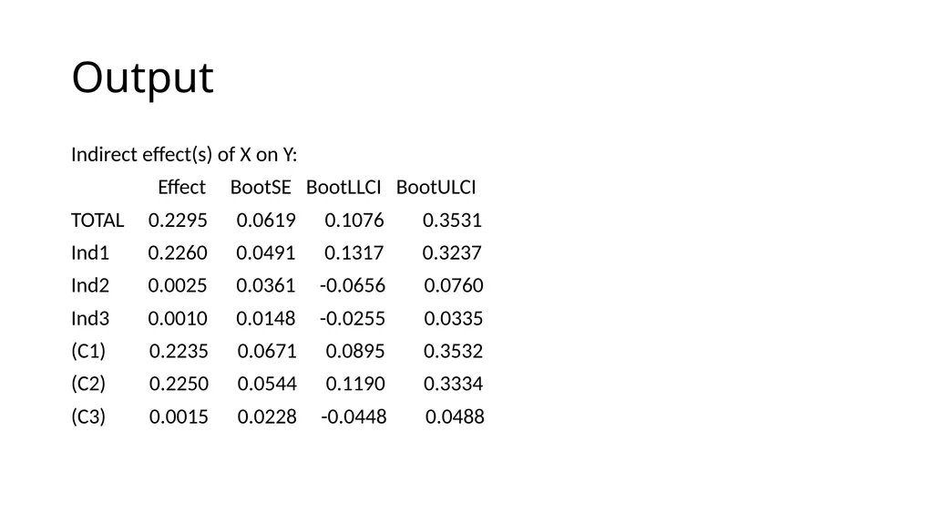
Output Indirect effect(s) of X on Y:
Effect BootSE BootLLCI BootULCI
TOTAL 0.2295 0.0619 0.1076 0.3531
Ind1 0.2260 0.0491 0.1317 0.3237
Ind2 0.0025 0.0361 -0.0656 0.0760
Ind3 0.0010 0.0148 -0.0255 0.0335
(C1) 0.2235 0.0671 0.0895 0.3532
(C2) 0.2250 0.0544 0.1190 0.3334
(C3) 0.0015 0.0228 -0.0448 0.0488<br>
Effect BootSE BootLLCI BootULCI
TOTAL 0.2295 0.0619 0.1076 0.3531
Ind1 0.2260 0.0491 0.1317 0.3237
Ind2 0.0025 0.0361 -0.0656 0.0760
Ind3 0.0010 0.0148 -0.0255 0.0335
(C1) 0.2235 0.0671 0.0895 0.3532
(C2) 0.2250 0.0544 0.1190 0.3334
(C3) 0.0015 0.0228 -0.0448 0.0488<br>
114
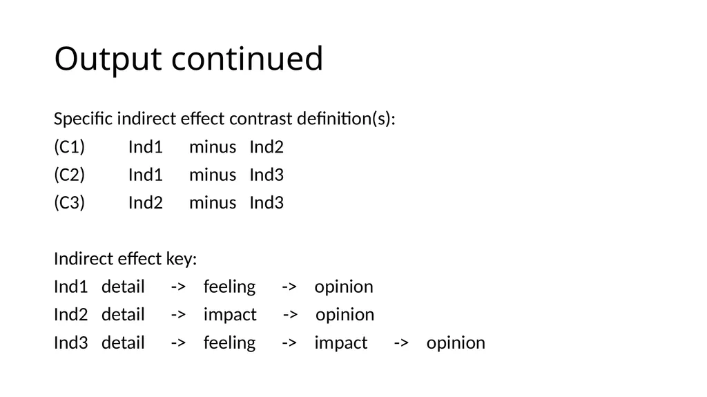
Output continued Specific indirect effect contrast definition(s):
(C1) Ind1 minus Ind2
(C2) Ind1 minus Ind3
(C3) Ind2 minus Ind3
Indirect effect key:
Ind1 detail -> feeling -> opinion
Ind2 detail -> impact -> opinion
Ind3 detail -> feeling -> impact -> opinion<br>
(C1) Ind1 minus Ind2
(C2) Ind1 minus Ind3
(C3) Ind2 minus Ind3
Indirect effect key:
Ind1 detail -> feeling -> opinion
Ind2 detail -> impact -> opinion
Ind3 detail -> feeling -> impact -> opinion<br>
115
Do you have any questions?<br>
116
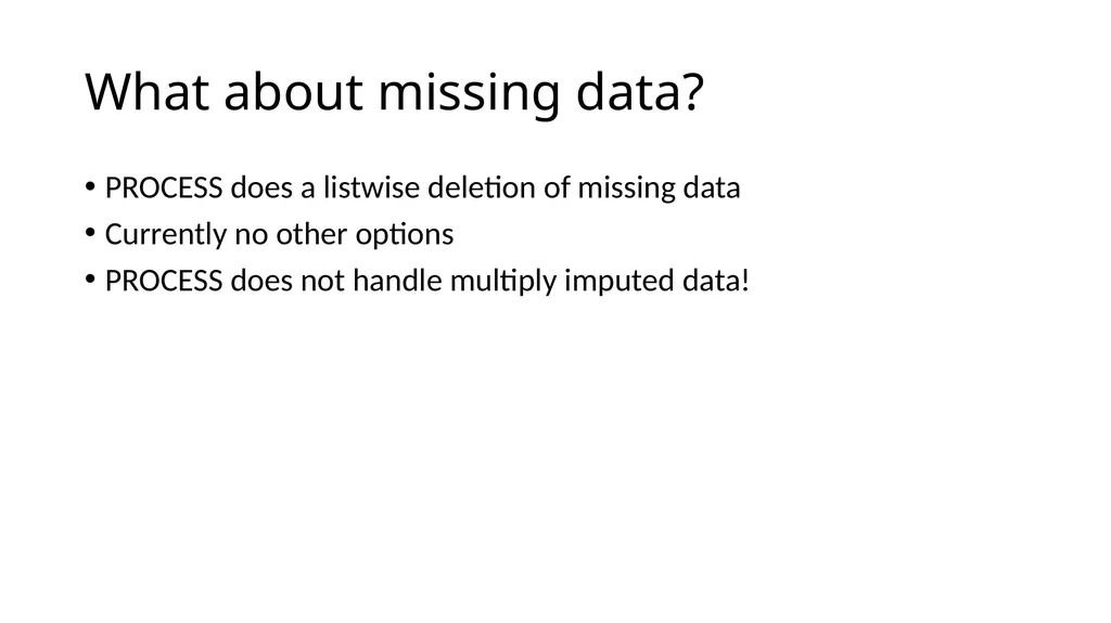
What about missing data? PROCESS does a listwise deletion of missing data
Currently no other options
PROCESS does not handle multiply imputed data!<br>
Currently no other options
PROCESS does not handle multiply imputed data!<br>
117
What about power and sample size? Usually explored with simulations
Not easy for several reasons
Little (if any) ready-to-use software
Usually need lots of data!<br>
Not easy for several reasons
Little (if any) ready-to-use software
Usually need lots of data!<br>
118
What to report See pages 542-544 for a complete discussion
Report all path coefficients and either their standard errors or CIs
It is not important if these are statistically significant
The sign of the path coefficients is important (because they impact the indirect effect, which is what you care about)
Report both the direct and indirect effect, as well as CIs and p-values
Avoid using the Sobel test
Provide some information about the bootstrapping
Number of bootstrapped samples and type of bootstrap (e.g., percentile, bias corrected, etc.)<br>
Report all path coefficients and either their standard errors or CIs
It is not important if these are statistically significant
The sign of the path coefficients is important (because they impact the indirect effect, which is what you care about)
Report both the direct and indirect effect, as well as CIs and p-values
Avoid using the Sobel test
Provide some information about the bootstrapping
Number of bootstrapped samples and type of bootstrap (e.g., percentile, bias corrected, etc.)<br>
119
What to report continued Be precise in the language used
Avoid “the indirect effect of M”
The effect of X on Y may go through M, but the quantity of interest is usually the indirect effect
No need to report percent mediated
The percent can exceed 100
The percent can be negative
See pages 148-151
Do not go through the Baron and Kenney “causal steps for mediation” as a precursor to the mediation analysis<br>
Avoid “the indirect effect of M”
The effect of X on Y may go through M, but the quantity of interest is usually the indirect effect
No need to report percent mediated
The percent can exceed 100
The percent can be negative
See pages 148-151
Do not go through the Baron and Kenney “causal steps for mediation” as a precursor to the mediation analysis<br>
120
Do you have any questions?<br>
121
Some subcommands available in PROCESS y: outcome variable (must be either continuous or binary)
x: predictor variable (may be continuous, binary or multicategorical)
m: mediator(s) (must be continuous)
w: first moderator
z: second moderator<br>
x: predictor variable (may be continuous, binary or multicategorical)
m: mediator(s) (must be continuous)
w: first moderator
z: second moderator<br>
122
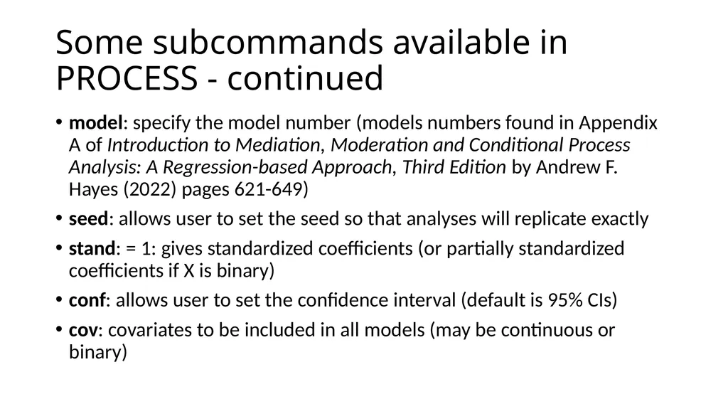
Some subcommands available in PROCESS - continued model: specify the model number (models numbers found in Appendix A of Introduction to Mediation, Moderation and Conditional Process Analysis: A Regression-based Approach, Third Edition by Andrew F. Hayes (2022) pages 621-649)
seed: allows user to set the seed so that analyses will replicate exactly
stand: = 1: gives standardized coefficients (or partially standardized coefficients if X is binary)
conf: allows user to set the confidence interval (default is 95% CIs)
cov: covariates to be included in all models (may be continuous or binary)<br>
seed: allows user to set the seed so that analyses will replicate exactly
stand: = 1: gives standardized coefficients (or partially standardized coefficients if X is binary)
conf: allows user to set the confidence interval (default is 95% CIs)
cov: covariates to be included in all models (may be continuous or binary)<br>
123
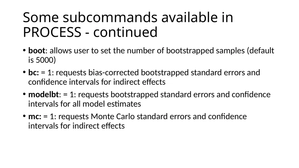
Some subcommands available in PROCESS - continued boot: allows user to set the number of bootstrapped samples (default is 5000)
bc: = 1: requests bias-corrected bootstrapped standard errors and confidence intervals for indirect effects
modelbt: = 1: requests bootstrapped standard errors and confidence intervals for all model estimates
mc: = 1: requests Monte Carlo standard errors and confidence intervals for indirect effects<br>
bc: = 1: requests bias-corrected bootstrapped standard errors and confidence intervals for indirect effects
modelbt: = 1: requests bootstrapped standard errors and confidence intervals for all model estimates
mc: = 1: requests Monte Carlo standard errors and confidence intervals for indirect effects<br>
124
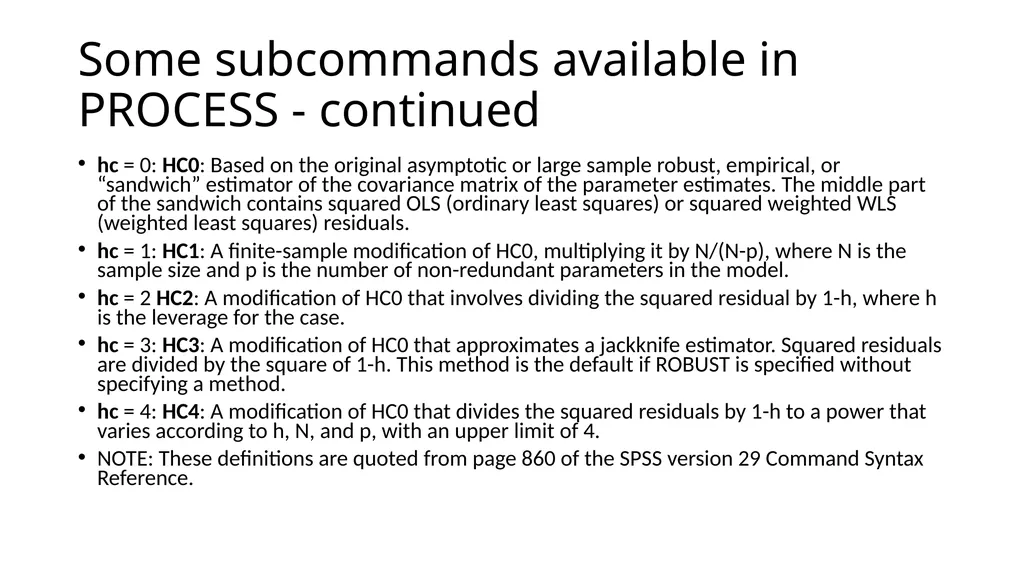
Some subcommands available in PROCESS - continued hc = 0: HC0: Based on the original asymptotic or large sample robust, empirical, or “sandwich” estimator of the covariance matrix of the parameter estimates. The middle part of the sandwich contains squared OLS (ordinary least squares) or squared weighted WLS (weighted least squares) residuals.
hc = 1: HC1: A finite-sample modification of HC0, multiplying it by N/(N-p), where N is the sample size and p is the number of non-redundant parameters in the model.
hc = 2 HC2: A modification of HC0 that involves dividing the squared residual by 1-h, where h is the leverage for the case.
hc = 3: HC3: A modification of HC0 that approximates a jackknife estimator. Squared residuals are divided by the square of 1-h. This method is the default if ROBUST is specified without specifying a method.
hc = 4: HC4: A modification of HC0 that divides the squared residuals by 1-h to a power that varies according to h, N, and p, with an upper limit of 4.
NOTE: These definitions are quoted from page 860 of the SPSS version 29 Command Syntax Reference.<br>
hc = 1: HC1: A finite-sample modification of HC0, multiplying it by N/(N-p), where N is the sample size and p is the number of non-redundant parameters in the model.
hc = 2 HC2: A modification of HC0 that involves dividing the squared residual by 1-h, where h is the leverage for the case.
hc = 3: HC3: A modification of HC0 that approximates a jackknife estimator. Squared residuals are divided by the square of 1-h. This method is the default if ROBUST is specified without specifying a method.
hc = 4: HC4: A modification of HC0 that divides the squared residuals by 1-h to a power that varies according to h, N, and p, with an upper limit of 4.
NOTE: These definitions are quoted from page 860 of the SPSS version 29 Command Syntax Reference.<br>
125
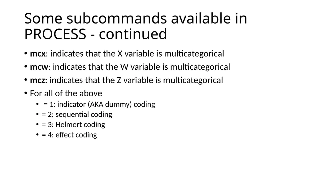
Some subcommands available in PROCESS - continued mcx: indicates that the X variable is multicategorical
mcw: indicates that the W variable is multicategorical
mcz: indicates that the Z variable is multicategorical
For all of the above
= 1: indicator (AKA dummy) coding
= 2: sequential coding
= 3: Helmert coding
= 4: effect coding<br>
mcw: indicates that the W variable is multicategorical
mcz: indicates that the Z variable is multicategorical
For all of the above
= 1: indicator (AKA dummy) coding
= 2: sequential coding
= 3: Helmert coding
= 4: effect coding<br>
126
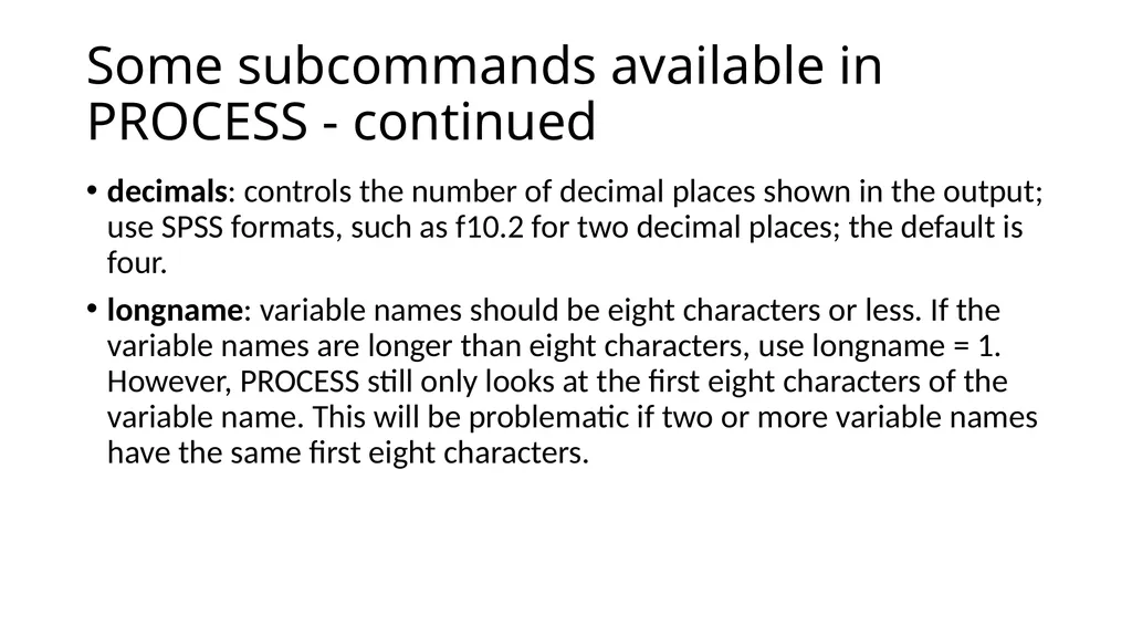
Some subcommands available in PROCESS - continued decimals: controls the number of decimal places shown in the output; use SPSS formats, such as f10.2 for two decimal places; the default is four.
longname: variable names should be eight characters or less. If the variable names are longer than eight characters, use longname = 1. However, PROCESS still only looks at the first eight characters of the variable name. This will be problematic if two or more variable names have the same first eight characters.<br>
longname: variable names should be eight characters or less. If the variable names are longer than eight characters, use longname = 1. However, PROCESS still only looks at the first eight characters of the variable name. This will be problematic if two or more variable names have the same first eight characters.<br>
127
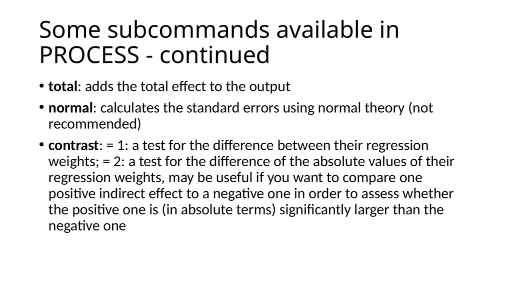
Some subcommands available in PROCESS - continued total: adds the total effect to the output
normal: calculates the standard errors using normal theory (not recommended)
contrast: = 1: a test for the difference between their regression weights; = 2: a test for the difference of the absolute values of their regression weights, may be useful if you want to compare one positive indirect effect to a negative one in order to assess whether the positive one is (in absolute terms) significantly larger than the negative one<br>
normal: calculates the standard errors using normal theory (not recommended)
contrast: = 1: a test for the difference between their regression weights; = 2: a test for the difference of the absolute values of their regression weights, may be useful if you want to compare one positive indirect effect to a negative one in order to assess whether the positive one is (in absolute terms) significantly larger than the negative one<br>
128
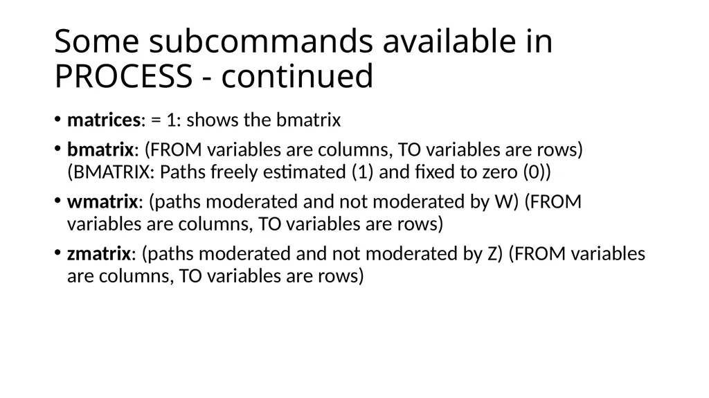
Some subcommands available in PROCESS - continued matrices: = 1: shows the bmatrix
bmatrix: (FROM variables are columns, TO variables are rows) (BMATRIX: Paths freely estimated (1) and fixed to zero (0))
wmatrix: (paths moderated and not moderated by W) (FROM variables are columns, TO variables are rows)
zmatrix: (paths moderated and not moderated by Z) (FROM variables are columns, TO variables are rows)<br>
bmatrix: (FROM variables are columns, TO variables are rows) (BMATRIX: Paths freely estimated (1) and fixed to zero (0))
wmatrix: (paths moderated and not moderated by W) (FROM variables are columns, TO variables are rows)
zmatrix: (paths moderated and not moderated by Z) (FROM variables are columns, TO variables are rows)<br>
129
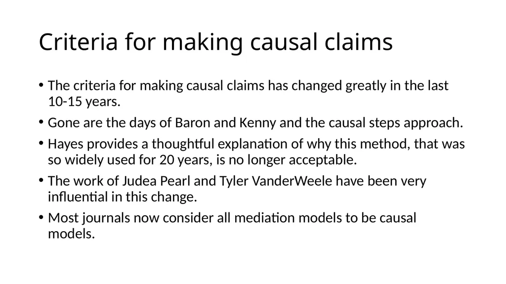
Criteria for making causal claims The criteria for making causal claims has changed greatly in the last 10-15 years.
Gone are the days of Baron and Kenny and the causal steps approach.
Hayes provides a thoughtful explanation of why this method, that was so widely used for 20 years, is no longer acceptable.
The work of Judea Pearl and Tyler VanderWeele have been very influential in this change.
Most journals now consider all mediation models to be causal models.<br>
Gone are the days of Baron and Kenny and the causal steps approach.
Hayes provides a thoughtful explanation of why this method, that was so widely used for 20 years, is no longer acceptable.
The work of Judea Pearl and Tyler VanderWeele have been very influential in this change.
Most journals now consider all mediation models to be causal models.<br>
130
A few considerations regarding causality The predictor must precede the mediator which must precede the outcome in time.
The cause must come before the effect.
This means that cross-sectional data are usually inappropriate for mediation analysis, because all of the data (for X, M and Y) are collected at the same time, so there is no way to guarantee that the cause happened before the effect.<br>
The cause must come before the effect.
This means that cross-sectional data are usually inappropriate for mediation analysis, because all of the data (for X, M and Y) are collected at the same time, so there is no way to guarantee that the cause happened before the effect.<br>
131
A few considerations regarding causality continued Just because you used a particular variable as the mediator does not mean that it is the only mediator.
Another variable might be the real mediator, and the variable you are using is just correlated with the real mediator.
A variable that is not in your model, and maybe not even in your dataset, causes both the mediator and the outcome.
When thinking about experiments and causality, most researchers immediately think of randomly assigning subjects to experimental groups or conditions; however, such assignment does not mean that mediator causes the outcome.<br>
Another variable might be the real mediator, and the variable you are using is just correlated with the real mediator.
A variable that is not in your model, and maybe not even in your dataset, causes both the mediator and the outcome.
When thinking about experiments and causality, most researchers immediately think of randomly assigning subjects to experimental groups or conditions; however, such assignment does not mean that mediator causes the outcome.<br>
132
Causal assumptions to be assessed In his paper Mediation Analysis: A Practitioner’s Guide (2015), VanderWeele lists four assumptions that need to be assessed so that the direct and indirect effects are interpretable.
no confounding between X and Y
no confounding between M and Y
no confounding between X and M
no confounding between M and Y that is itself affected by X.<br>
no confounding between X and Y
no confounding between M and Y
no confounding between X and M
no confounding between M and Y that is itself affected by X.<br>
133
Any last questions??<br>
134
Thank you!<br>