04
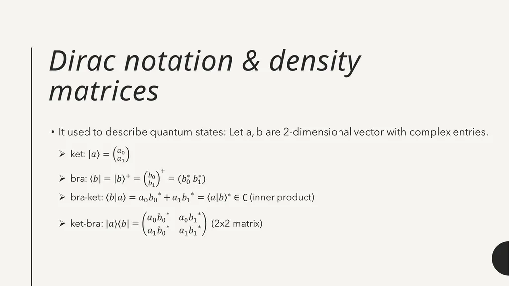
Dirac notation & density matrices<br>
05
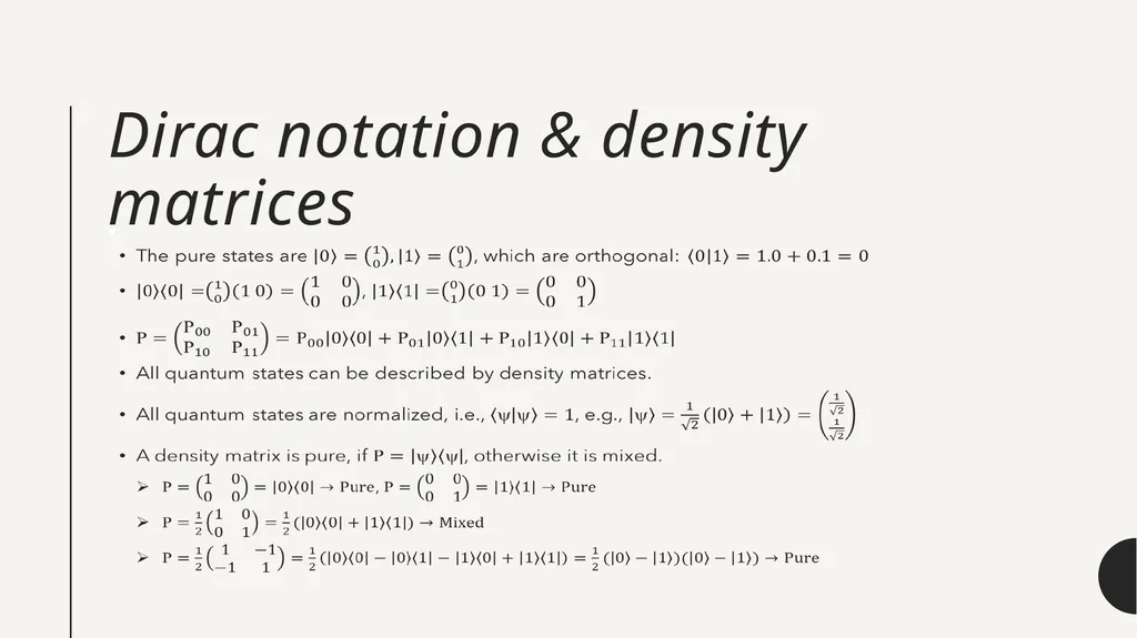
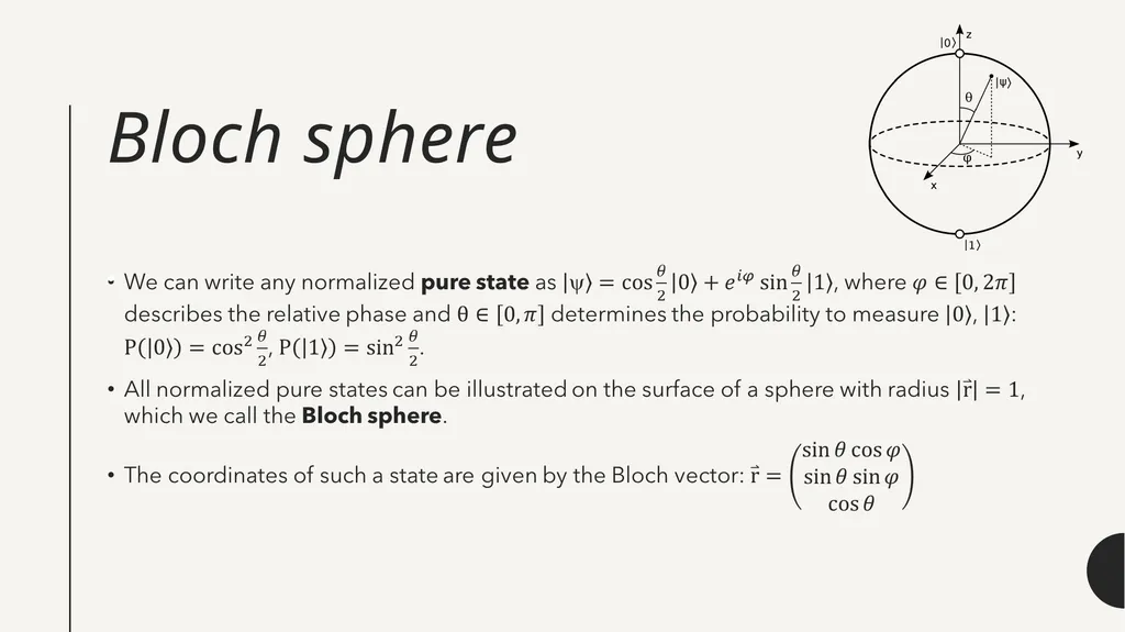
Dirac notation & density matrices<br>
09
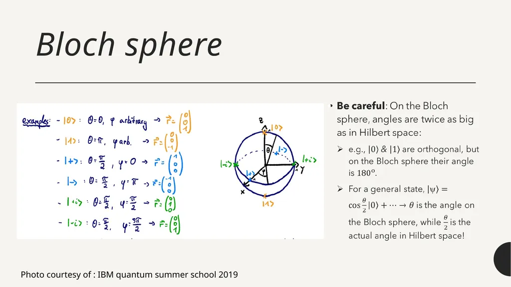
Bloch sphere Photo courtesy of : IBM quantum summer school 2019<br>
10
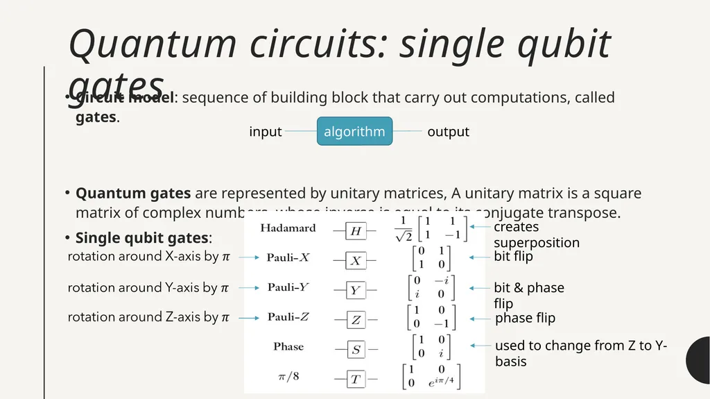
Quantum circuits: single qubit gates Circuit model: sequence of building block that carry out computations, called gates.
Quantum gates are represented by unitary matrices, A unitary matrix is a square matrix of complex numbers, whose inverse is equal to its conjugate transpose.
Single qubit gates: algorithm input output bit flip phase flip bit & phase flip creates superposition used to change from Z to Y-basis<br>
11
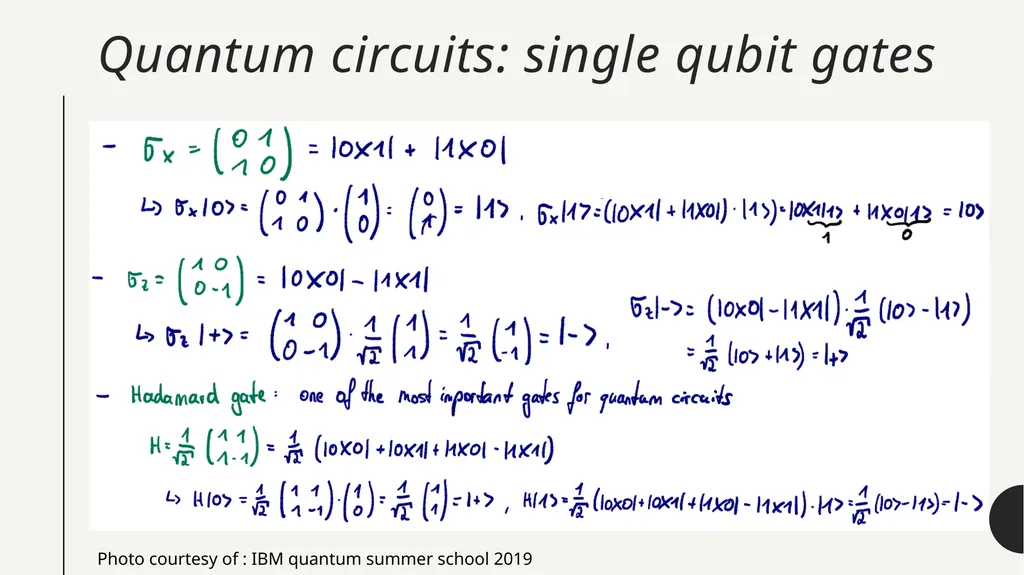
Quantum circuits: single qubit gates Photo courtesy of : IBM quantum summer school 2019<br>
12
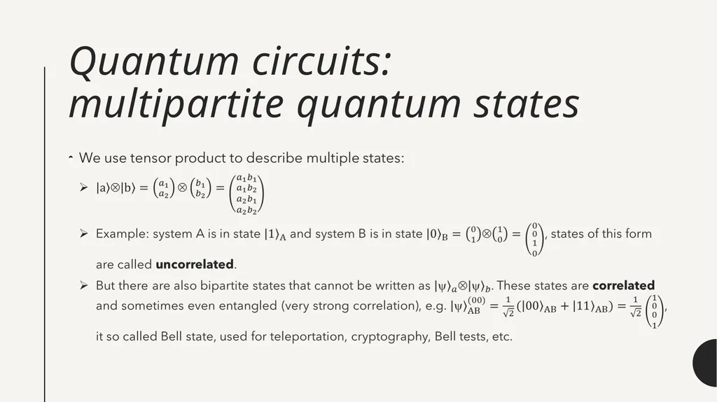
Quantum circuits: �multipartite quantum states<br>
13
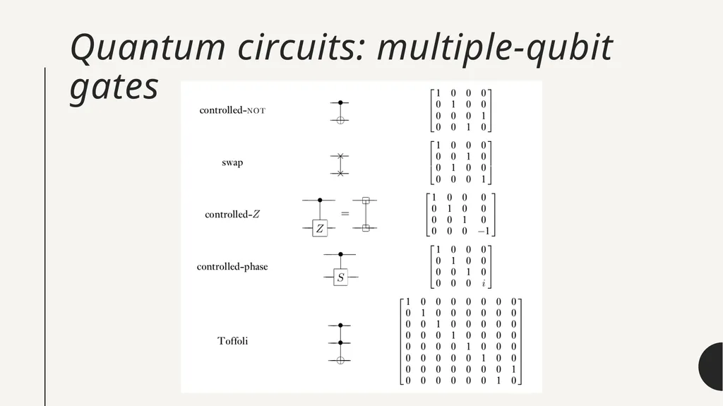
Quantum circuits: multiple-qubit gates<br>
14
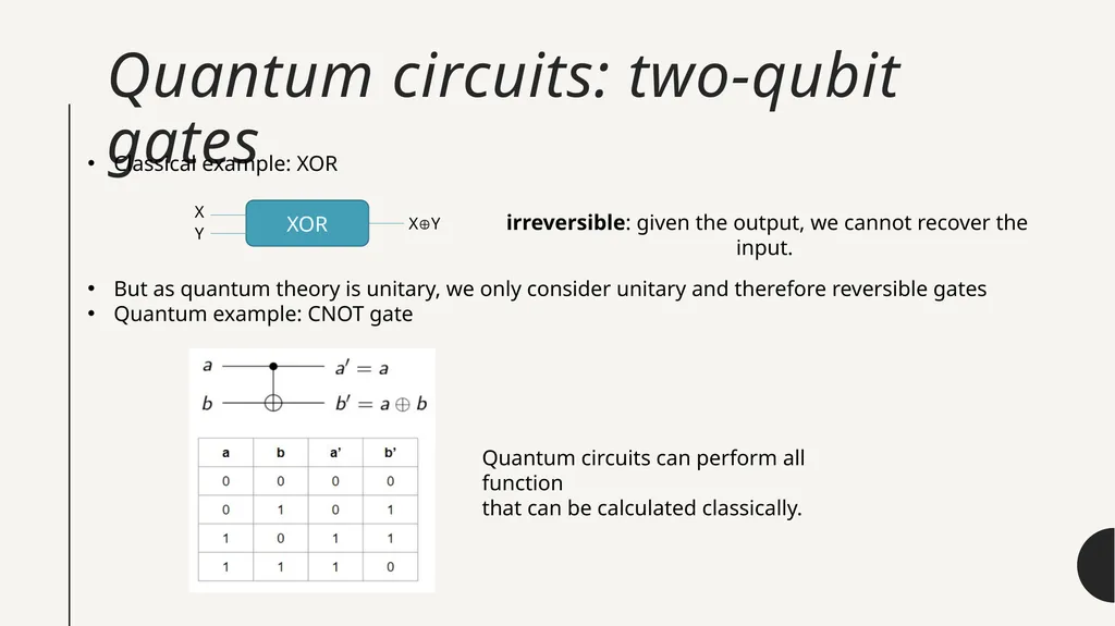
Quantum circuits: two-qubit gates Classical example: XOR
But as quantum theory is unitary, we only consider unitary and therefore reversible gates
Quantum example: CNOT gate XOR X Y XY irreversible: given the output, we cannot recover the input. Quantum circuits can perform all function
that can be calculated classically.<br>
17
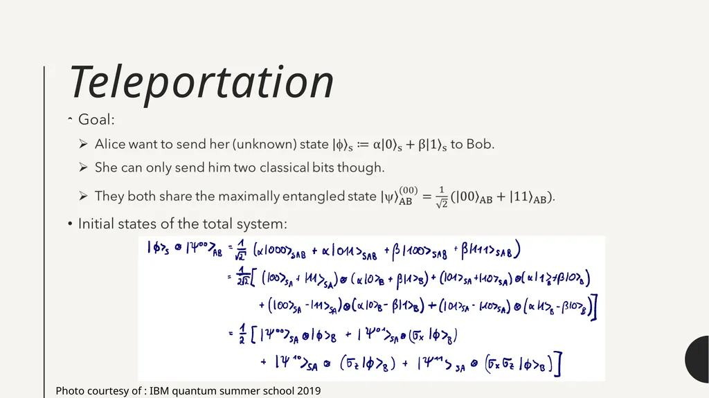
Teleportation Photo courtesy of : IBM quantum summer school 2019<br>
18
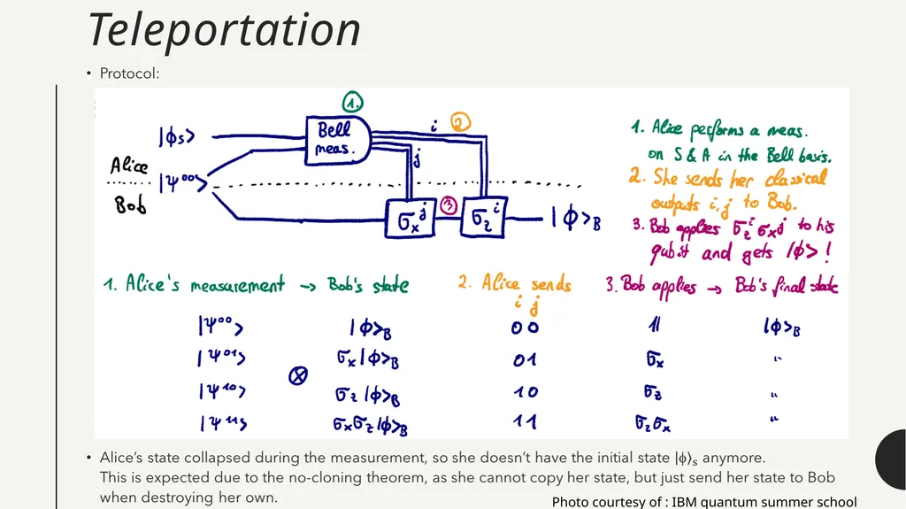
Teleportation Photo courtesy of : IBM quantum summer school 2019<br>
19
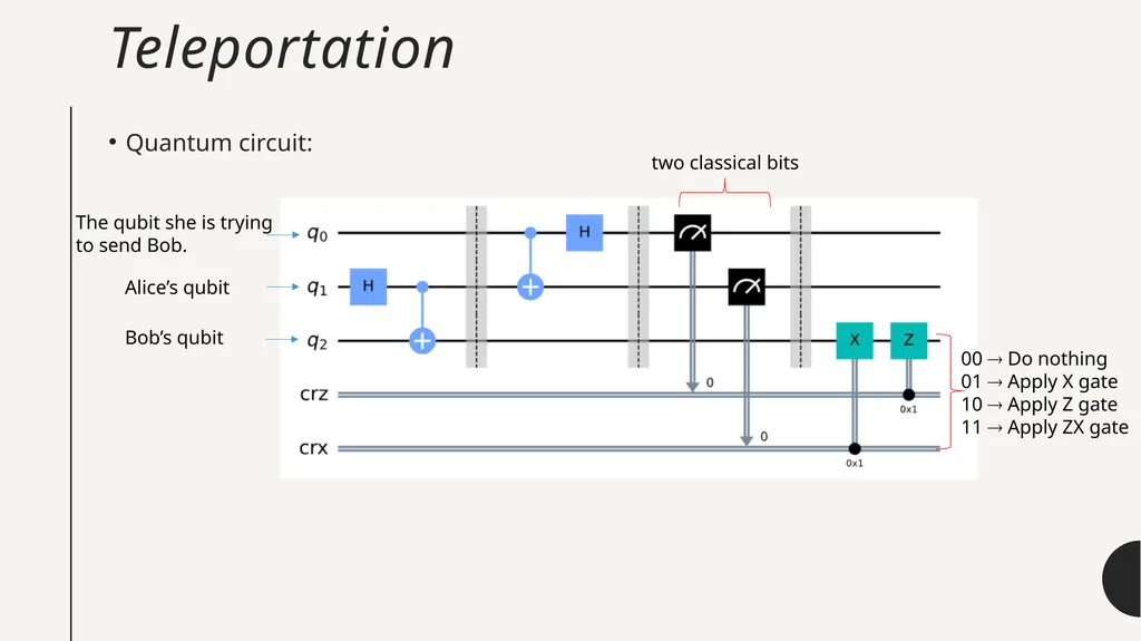
Teleportation Quantum circuit: Alice’s qubit Bob’s qubit The qubit she is trying to send Bob. two classical bits 00 Do nothing
01 Apply X gate
10 Apply Z gate
11 Apply ZX gate<br>
20
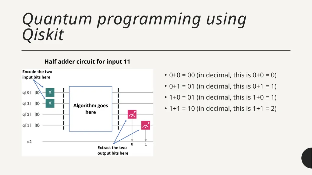
Quantum programming using Qiskit 0+0 = 00 (in decimal, this is 0+0 = 0)
0+1 = 01 (in decimal, this is 0+1 = 1)
1+0 = 01 (in decimal, this is 1+0 = 1)
1+1 = 10 (in decimal, this is 1+1 = 2) Half adder circuit for input 11<br>
21
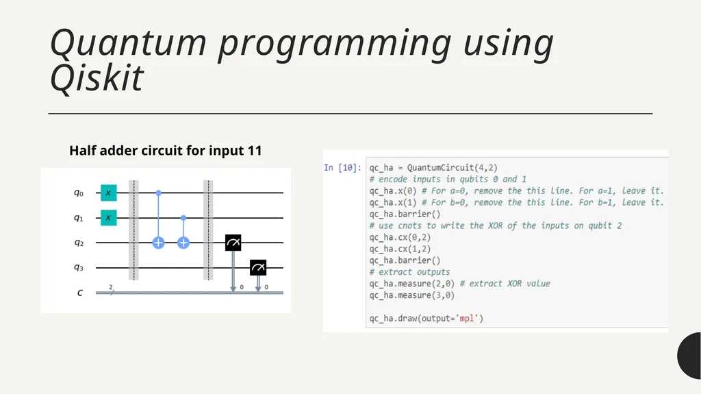
Quantum programming using Qiskit Half adder circuit for input 11<br>
22
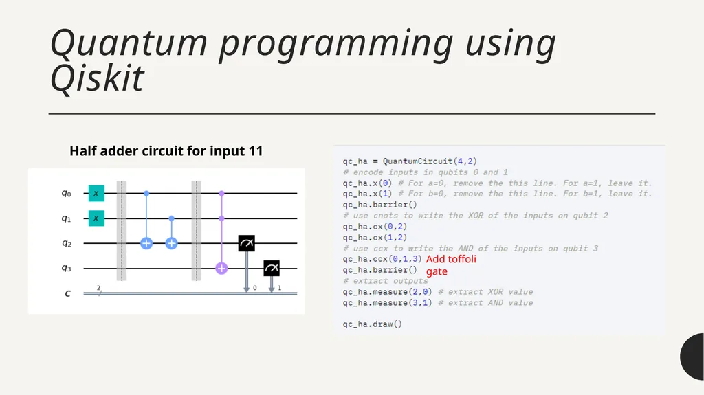
Quantum programming using Qiskit Half adder circuit for input 11 Add toffoli gate<br>
23
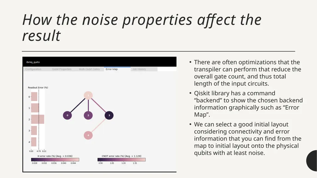
How the noise properties affect the result There are often optimizations that the transpiler can perform that reduce the overall gate count, and thus total length of the input circuits.
Qiskit library has a command “backend” to show the chosen backend information graphically such as “Error Map”.
We can select a good initial layout considering connectivity and error information that you can find from the map to initial layout onto the physical qubits with at least noise.<br>
24
Assignment I: quantum circuits Required:
Go to https://quantum-computing.ibm.com/
Register IBMid account or sign in with Google, Github, LinkedIn, and Twitter.
Download source codes at t.ly/M8Qg and upload files “Lab-1.ipynb” and “Lab-2.ipynb” into IBM Quantum Lab.<br>
25
Quantum algorithms Deutsch-Jozsa algorithm
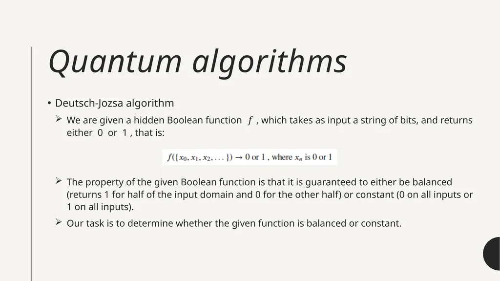
We are given a hidden Boolean function 𝑓 , which takes as input a string of bits, and returns either 0 or 1 , that is:
The property of the given Boolean function is that it is guaranteed to either be balanced (returns 1 for half of the input domain and 0 for the other half) or constant (0 on all inputs or 1 on all inputs).
Our task is to determine whether the given function is balanced or constant.<br>
26
Quantum algorithms Deutsch-Jozsa algorithm
For classical solution, we need to ask the oracle at least twice, but if we get twice the same output, we need to ask again. At most to query is (N/2)+1, where N is number of state.
For quantum solution, need only one query. If the output is the zero bit string, we know that the oracle is constant. If it is any other bit string, we know that it is balanced.
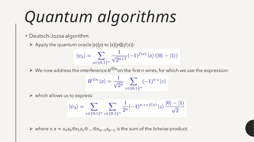
We have the function 𝑓 implemented as a quantum oracle, which maps the state |𝑥⟩|𝑦⟩ to |𝑥⟩|𝑦⊕𝑓(𝑥)⟩ , where ⊕ is addition modulo 2.<br>
27
Quantum algorithms Deutsch-Jozsa algorithm
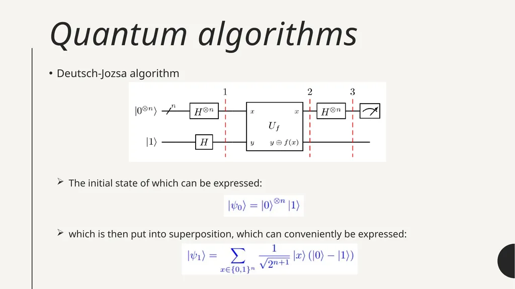
The initial state of which can be expressed:
which is then put into superposition, which can conveniently be expressed:<br>
28
Quantum algorithms<br>
29
Quantum algorithms Deutsch-Jozsa algorithm
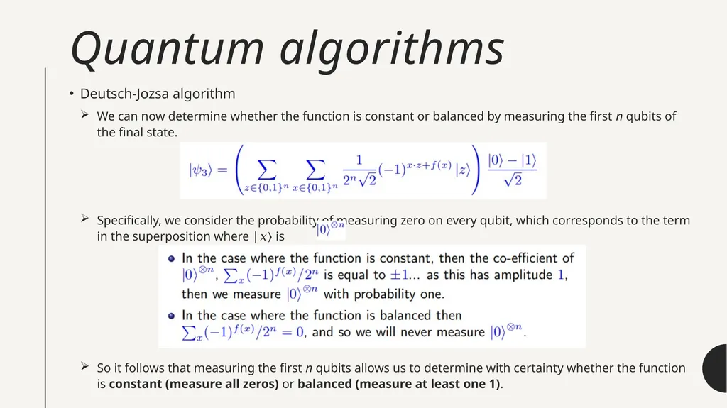
We can now determine whether the function is constant or balanced by measuring the first n qubits of the final state.
Specifically, we consider the probability of measuring zero on every qubit, which corresponds to the term in the superposition where |𝑥⟩ is
So it follows that measuring the first n qubits allows us to determine with certainty whether the function is constant (measure all zeros) or balanced (measure at least one 1).<br>
30
Quantum algorithms Deutsch-Jozsa algorithm
We can encode any mathematical function as a unitary matrix.
Deutsch’s algorithm was the first algorithm that demonstrated a quantum advantage: specifically, a reduction in query complexity compared to the classical case.
The Deutsch-Jozsa algorithm generalises Deutsch’s algorithm and reveals the possibility of exponential speed-ups using quantum computers.<br>
31
Assignment II: quantum algorithms Required:
Go to https://quantum-computing.ibm.com/
Download source codes at t.ly/M8Qg and upload files “Lab-3.ipynb” into IBM Quantum Lab.<br>
32
Quantum algorithms Grover’s algorithm
It can be used to solve unstructured search problems.
This algorithm can speed up an unstructured search problem quadratically using the amplitude amplification trick.<br>
33
Quantum algorithms Grover’s algorithm
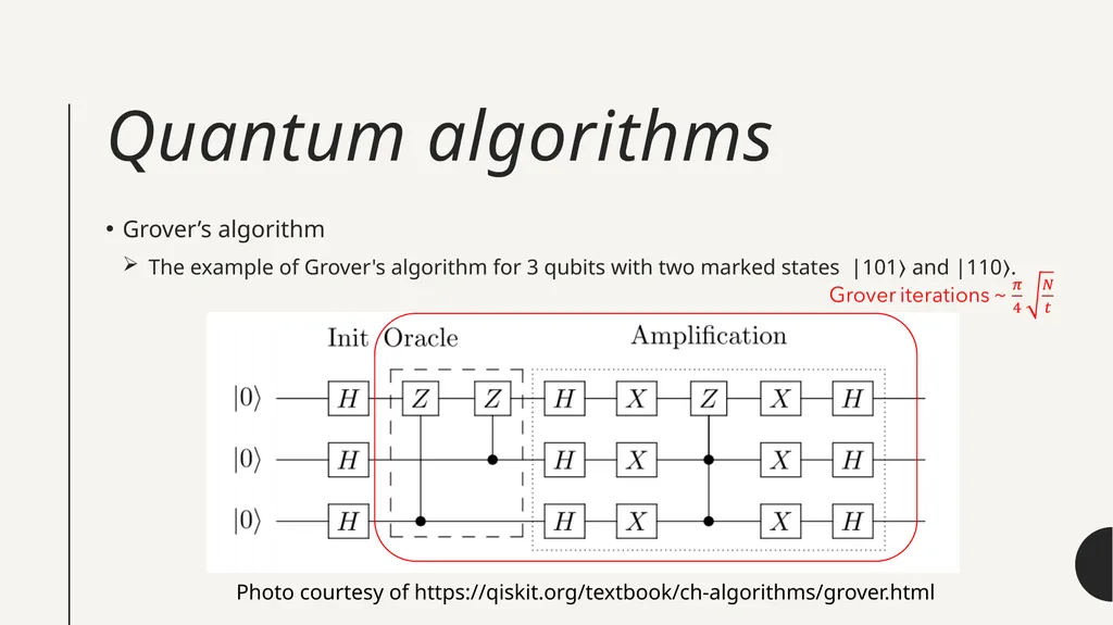
The example of Grover's algorithm for 3 qubits with two marked states |101⟩ and |110⟩. Photo courtesy of https://qiskit.org/textbook/ch-algorithms/grover.html<br>
34
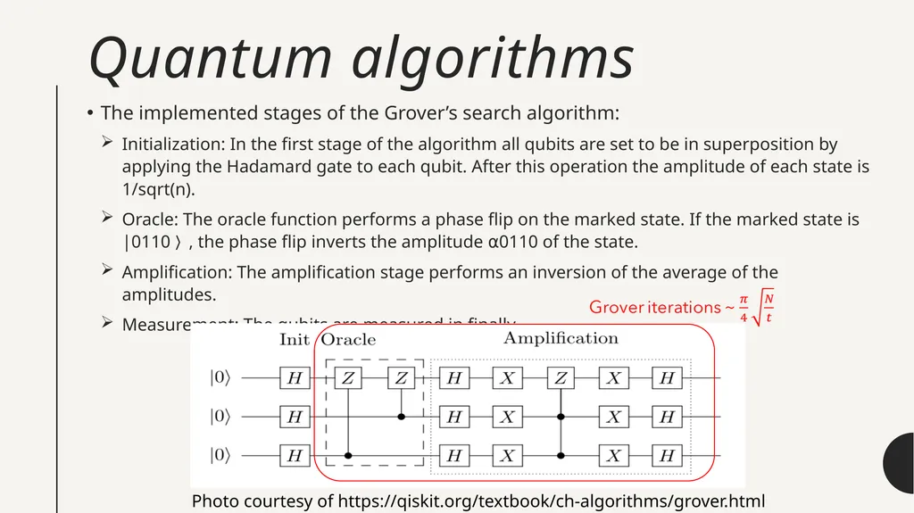
Quantum algorithms The implemented stages of the Grover’s search algorithm:
Initialization: In the first stage of the algorithm all qubits are set to be in superposition by applying the Hadamard gate to each qubit. After this operation the amplitude of each state is 1/sqrt(n).
Oracle: The oracle function performs a phase flip on the marked state. If the marked state is |0110〉, the phase flip inverts the amplitude ⍺0110 of the state.
Amplification: The amplification stage performs an inversion of the average of the amplitudes.
Measurement: The qubits are measured in finally. Photo courtesy of https://qiskit.org/textbook/ch-algorithms/grover.html<br>
35
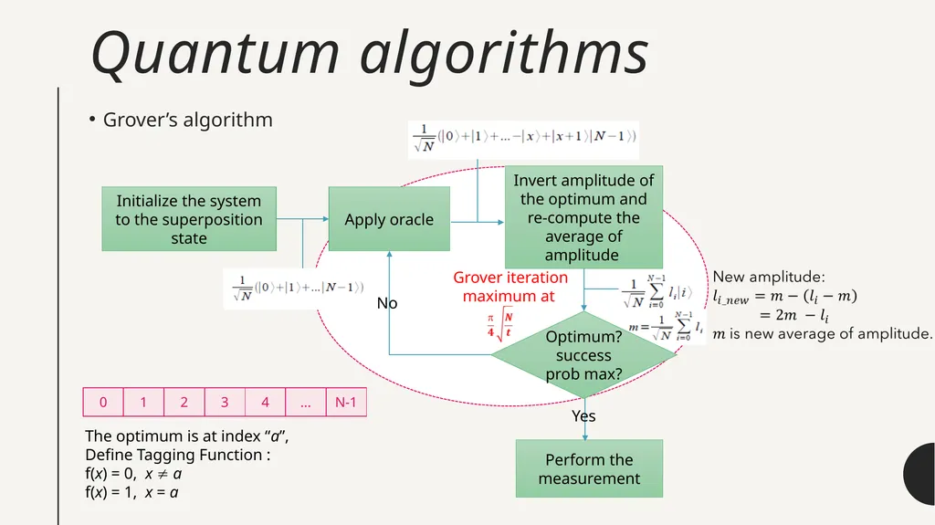
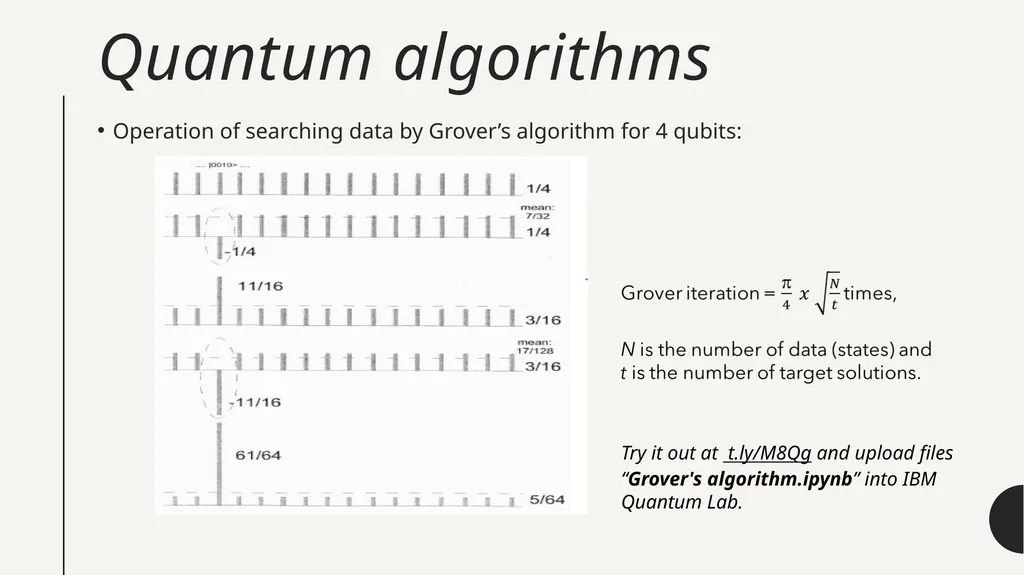
Quantum algorithms Grover’s algorithm Grover iteration�maximum at Initialize the system to the superposition state Apply oracle Invert amplitude of the optimum and re-compute the average of amplitude Perform the measurement No Yes Optimum? success prob max? The optimum is at index “a”,
Define Tagging Function :
f(x) = 0, x a
f(x) = 1, x = a<br>
36
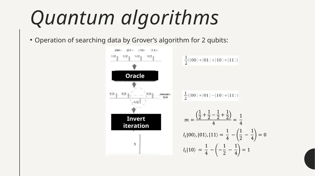
Quantum algorithms Operation of searching data by Grover’s algorithm for 2 qubits:<br>
37
Quantum algorithms Operation of searching data by Grover’s algorithm for 4 qubits: Try it out at t.ly/M8Qg and upload files “Grover's algorithm.ipynb” into IBM Quantum Lab.<br>
38
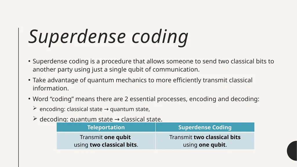
Superdense coding Superdense coding is a procedure that allows someone to send two classical bits to another party using just a single qubit of communication.
Take advantage of quantum mechanics to more efficiently transmit classical information.
Word “coding” means there are 2 essential processes, encoding and decoding:
encoding: classical state → quantum state,
decoding: quantum state → classical state.<br>
39
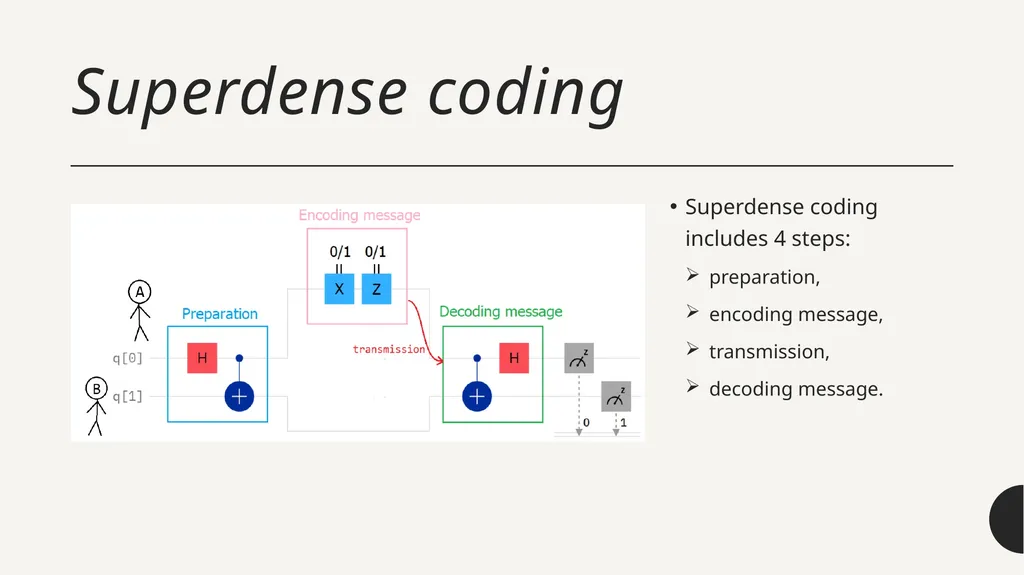
Superdense coding Superdense coding includes 4 steps:
preparation,
encoding message,
transmission,
decoding message.<br>
40
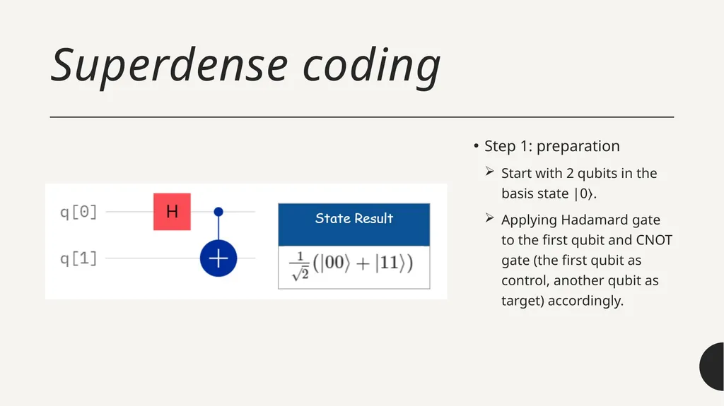
Superdense coding Step 1: preparation
Start with 2 qubits in the basis state |0⟩.
Applying Hadamard gate to the first qubit and CNOT gate (the first qubit as control, another qubit as target) accordingly.<br>
41
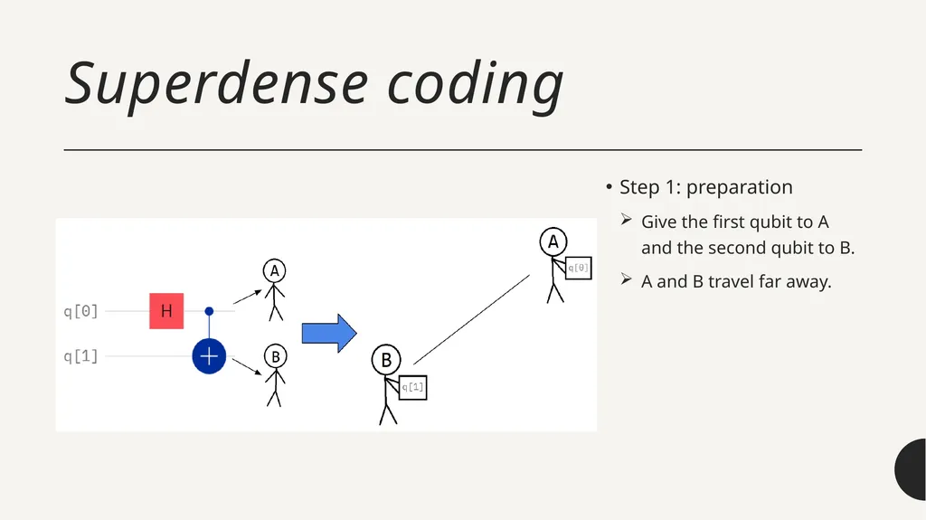
Superdense coding Step 1: preparation
Give the first qubit to A and the second qubit to B.
A and B travel far away.<br>
42
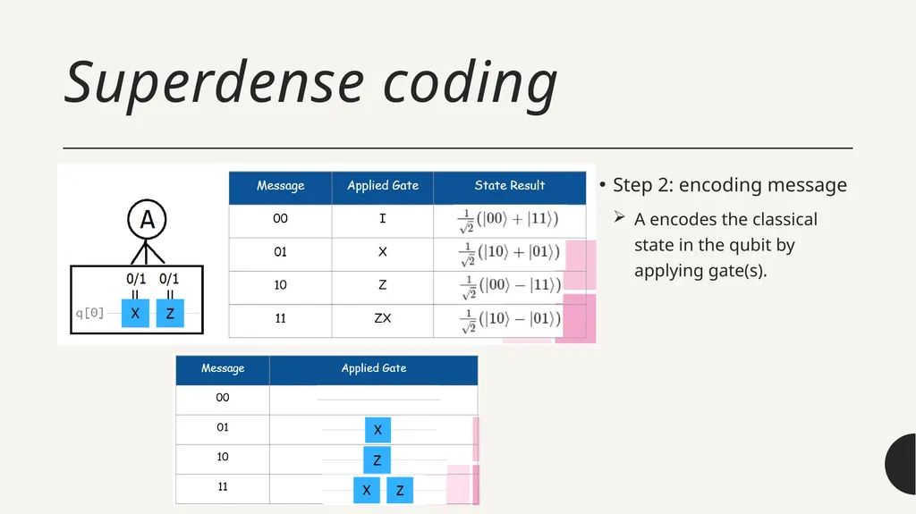
Superdense coding Step 2: encoding message
A encodes the classical state in the qubit by applying gate(s).<br>
43
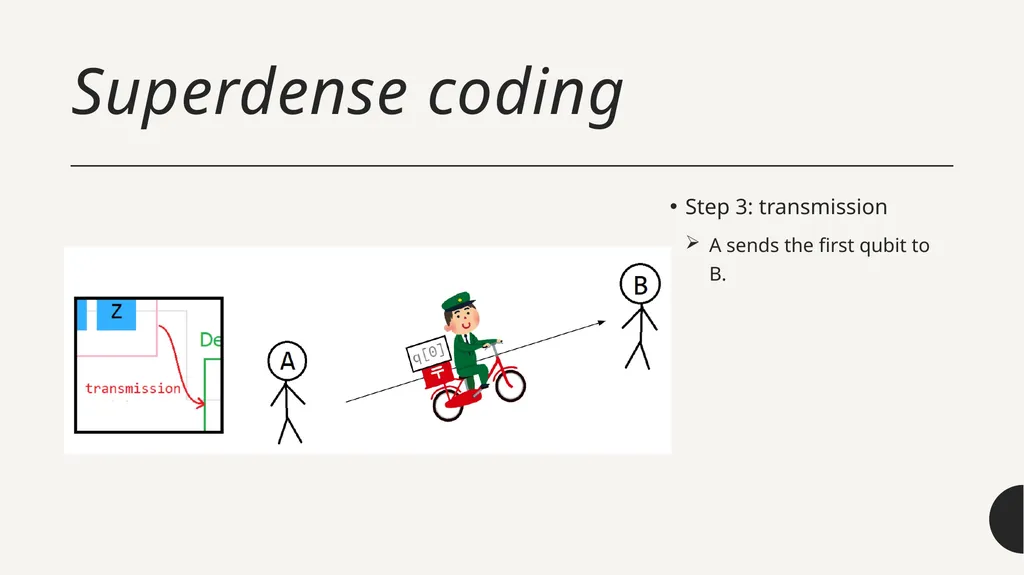
Superdense coding Step 3: transmission
A sends the first qubit to B.<br>
44
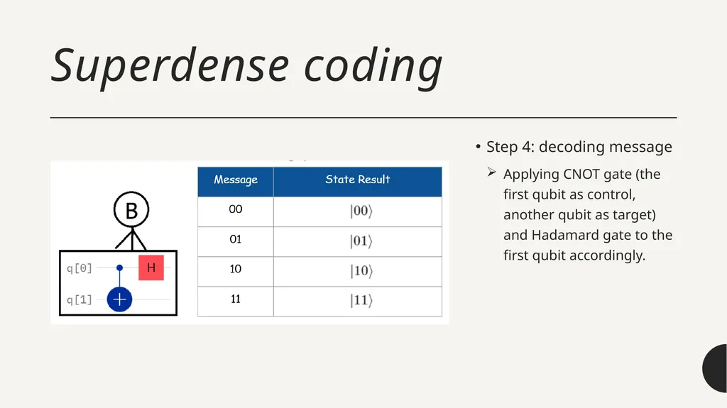
Superdense coding Step 4: decoding message
Applying CNOT gate (the first qubit as control, another qubit as target) and Hadamard gate to the first qubit accordingly.<br>
45
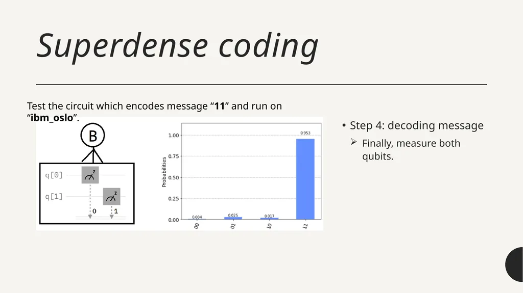
Superdense coding Step 4: decoding message
Finally, measure both qubits. Test the circuit which encodes message “11” and run on “ibm_oslo”.<br>
46
Assignment II: superdense coding Required:
Go to https://quantum-computing.ibm.com/
Download source codes at t.ly/M8Qg and upload files “Lab-4.ipynb” into IBM Quantum Lab.<br>