Latent Tree Models Part IV: Applications Nevin L.

slide1. Latent Tree ModelsPart IV: Applications Nevin L. Zhang
Dept. of Computer Science & Engineering
The Hong Kong Univ. of Sci. & Tech.
http://www.cse.ust.hk/~lzhang AAAI 2014 Tutorial<br>
slide2. What can LTA be used for:
Discovery of co-occurrence patterns in binary data
Discovery of correlation patterns in general discrete data
Discovery of latent variable/structures
Multidimensional clustering
Topic detection in text data
Probabilistic modelling

Applications
Analysis of survey data
Market survey data, social survey, medical survey data
Analysis of text data
Topic detection
Approximate probabilistic inference Applications of Latent Tree Analysis (LTA)<br>
slide3. Part IV: Applications Approximate Inference in Bayesian Networks

Analysis of social survey data

Topic detection in text data

Analysis of medical symptom survey data

Software<br>
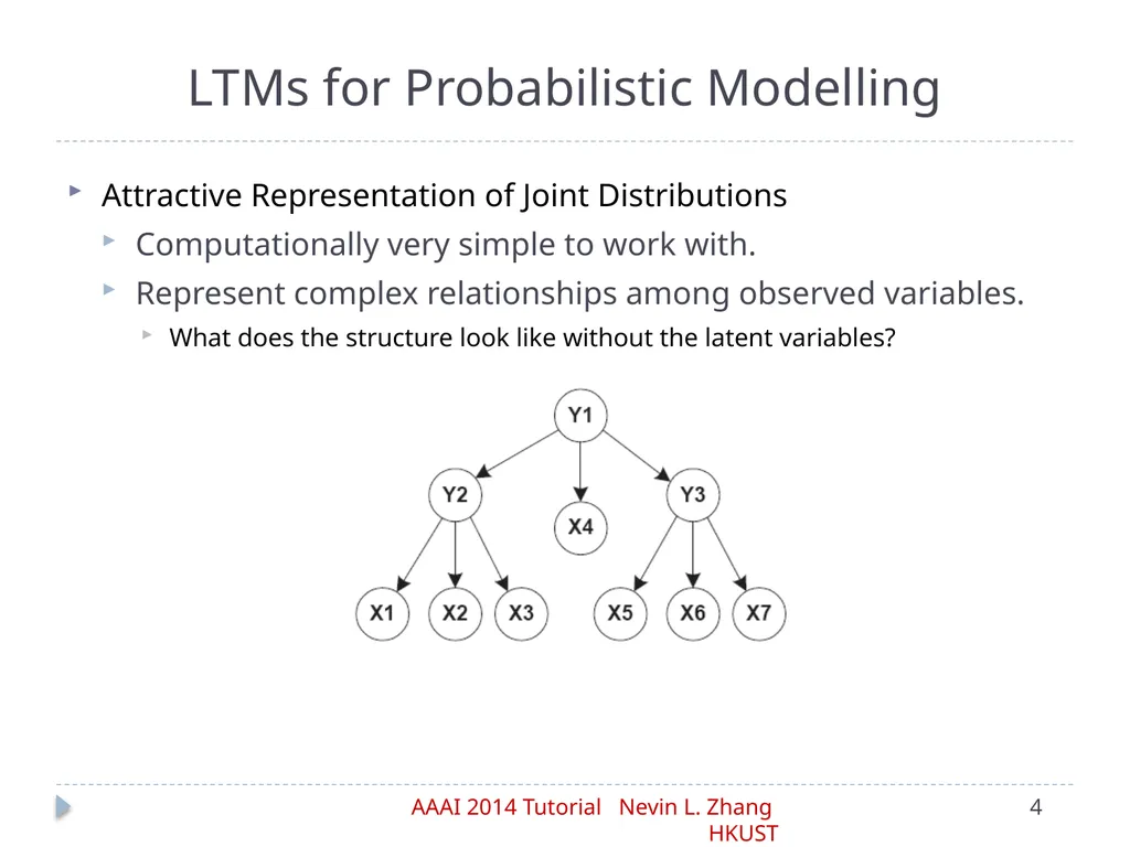
slide4. Attractive Representation of Joint Distributions
Computationally very simple to work with.
Represent complex relationships among observed variables.
What does the structure look like without the latent variables? LTMs for Probabilistic Modelling<br>
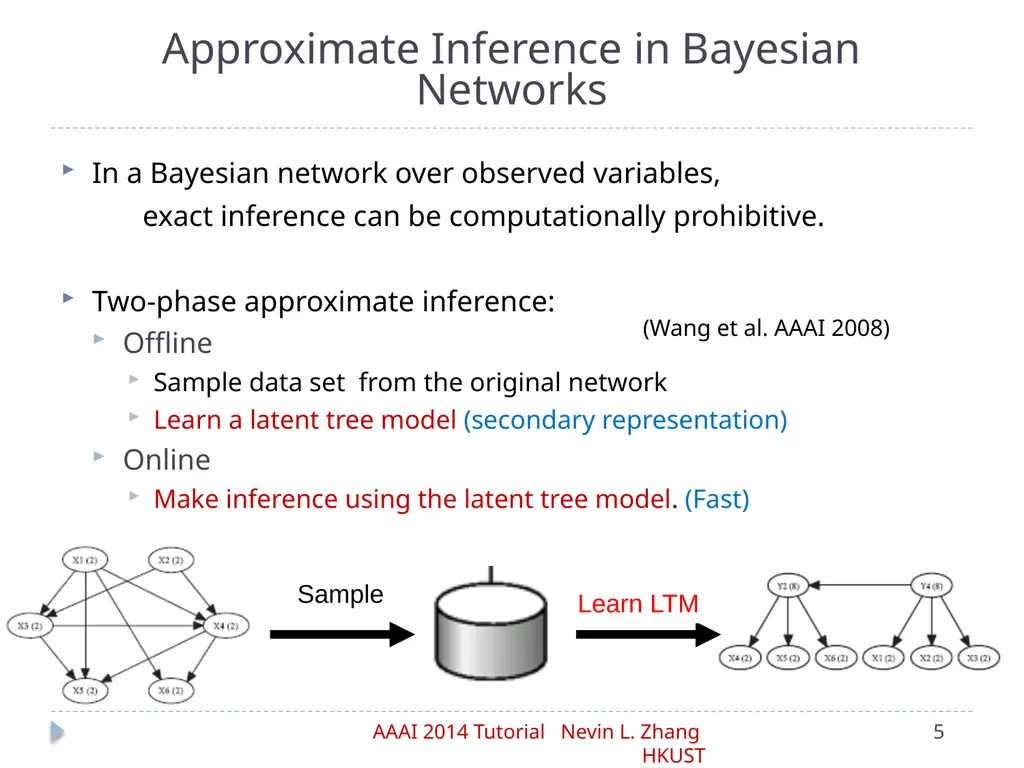
slide5. In a Bayesian network over observed variables,
exact inference can be computationally prohibitive.

Two-phase approximate inference:
Offline
Sample data set from the original network
Learn a latent tree model (secondary representation)
Online
Make inference using the latent tree model. (Fast) Approximate Inference in Bayesian Networks (Wang et al. AAAI 2008)<br>
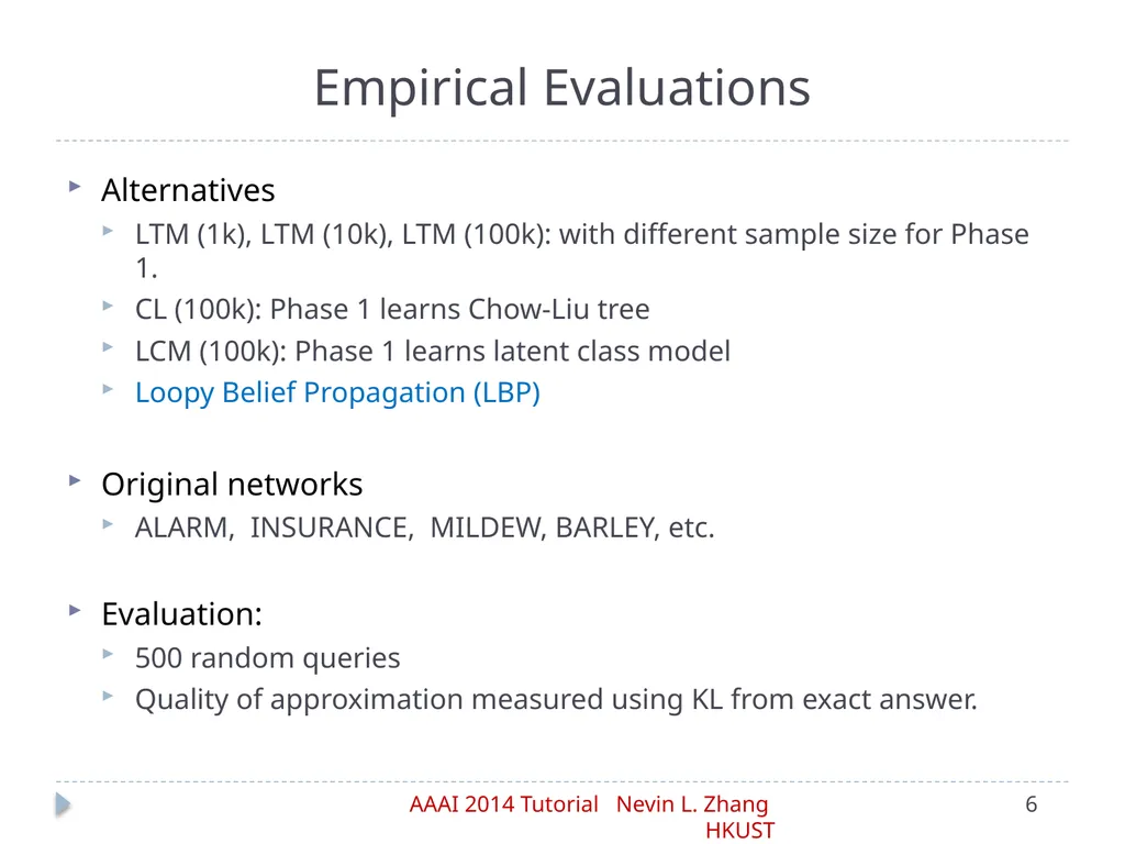
slide6. Alternatives
LTM (1k), LTM (10k), LTM (100k): with different sample size for Phase 1.
CL (100k): Phase 1 learns Chow-Liu tree
LCM (100k): Phase 1 learns latent class model
Loopy Belief Propagation (LBP)

Original networks
ALARM, INSURANCE, MILDEW, BARLEY, etc.

Evaluation:
500 random queries
Quality of approximation measured using KL from exact answer. Empirical Evaluations<br>
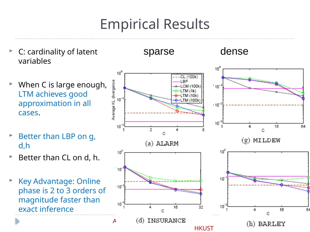
slide7. C: cardinality of latent variables

When C is large enough, LTM achieves good approximation in all cases.

Better than LBP on g, d,h
Better than CL on d, h.

Key Advantage: Online phase is 2 to 3 orders of magnitude faster than exact inference Empirical Results sparse dense<br>
slide8. Part III: Applications Approximate Inference in Bayesian networks

Analysis of social survey data

Topic detection

Analysis of medical symptom survey data

Software<br>
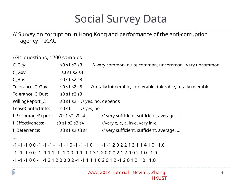
slide9. Social Survey Data // Survey on corruption in Hong Kong and performance of the anti-corruption agency -- ICAC

//31 questions, 1200 samples
C_City: s0 s1 s2 s3 // very common, quite common, uncommon, very uncommon
C_Gov: s0 s1 s2 s3
C_Bus: s0 s1 s2 s3
Tolerance_C_Gov: s0 s1 s2 s3 //totally intolerable, intolerable, tolerable, totally tolerable
Tolerance_C_Bus: s0 s1 s2 s3
WillingReport_C: s0 s1 s2 // yes, no, depends
LeaveContactInfo: s0 s1 // yes, no
I_EncourageReport: s0 s1 s2 s3 s4 // very sufficient, sufficient, average, ...
I_Effectiveness: s0 s1 s2 s3 s4 //very e, e, a, in-e, very in-e
I_Deterrence: s0 s1 s2 s3 s4 // very sufficient, sufficient, average, ...
…..
-1 -1 -1 0 0 -1 -1 -1 -1 -1 -1 0 -1 -1 -1 0 1 1 -1 -1 2 0 2 2 1 3 1 1 4 1 0 1.0
-1 -1 -1 0 0 -1 -1 1 1 -1 -1 0 0 -1 1 -1 1 3 2 2 0 0 0 2 1 2 0 0 2 1 0 1.0
-1 -1 -1 0 0 -1 -1 2 1 2 0 0 0 2 -1 -1 1 1 1 0 2 0 1 2 -1 2 0 1 2 1 0 1.0
….<br>
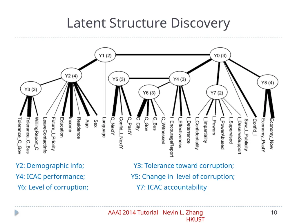
slide10. Latent Structure Discovery Y2: Demographic info; Y3: Tolerance toward corruption;
Y4: ICAC performance; Y5: Change in level of corruption;
Y6: Level of corruption; Y7: ICAC accountability<br>
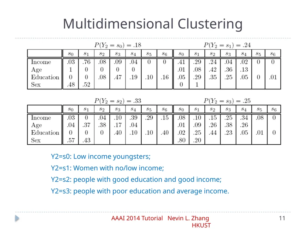
slide11. Multidimensional Clustering Y2=s0: Low income youngsters;
Y2=s1: Women with no/low income;
Y2=s2: people with good education and good income;
Y2=s3: people with poor education and average income.<br>
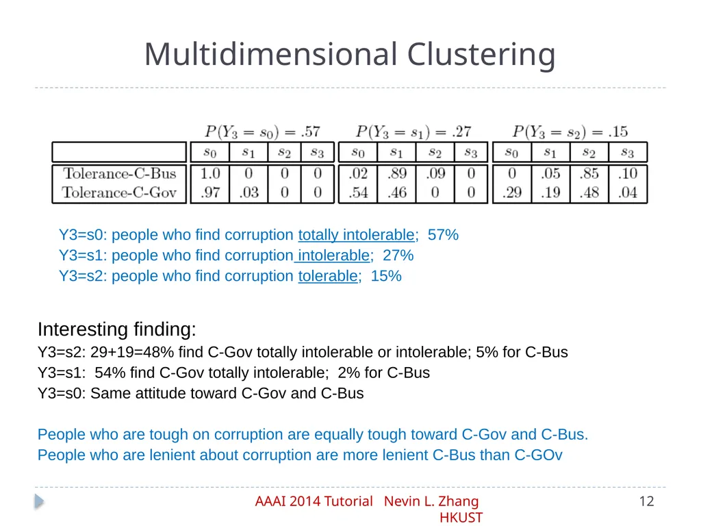
slide12. Multidimensional Clustering Y3=s0: people who find corruption totally intolerable; 57%
Y3=s1: people who find corruption intolerable; 27%
Y3=s2: people who find corruption tolerable; 15% Interesting finding:
Y3=s2: 29+19=48% find C-Gov totally intolerable or intolerable; 5% for C-Bus
Y3=s1: 54% find C-Gov totally intolerable; 2% for C-Bus
Y3=s0: Same attitude toward C-Gov and C-Bus

People who are tough on corruption are equally tough toward C-Gov and C-Bus.
People who are lenient about corruption are more lenient C-Bus than C-GOv<br>
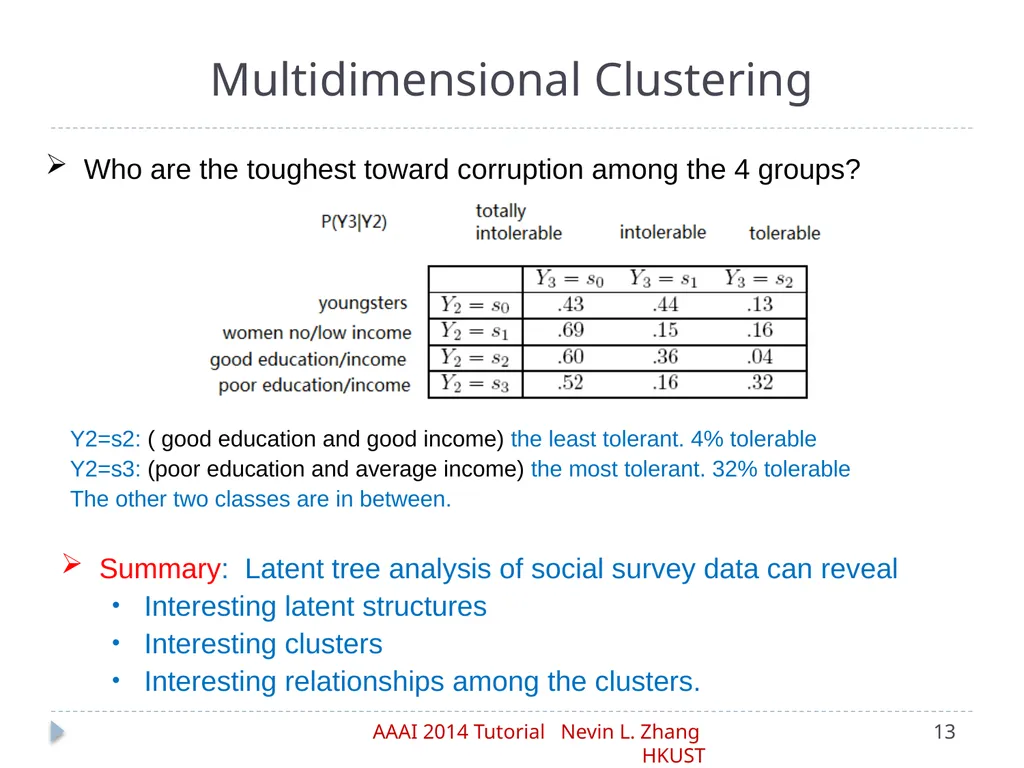
slide13. Multidimensional Clustering Who are the toughest toward corruption among the 4 groups? Y2=s2: ( good education and good income) the least tolerant. 4% tolerable
Y2=s3: (poor education and average income) the most tolerant. 32% tolerable
The other two classes are in between. Summary: Latent tree analysis of social survey data can reveal
Interesting latent structures
Interesting clusters
Interesting relationships among the clusters.<br>
slide14. Part III: Applications Approximate Inference

Analysis of social survey data

Topic detection (Analysis of text data)

Analysis of medical symptom survey data

Software<br>
slide15. Basics

Aggregation of miniature topics

Topic extraction and characterization

Empirical results Latent Tree Models for Topic Detection<br>
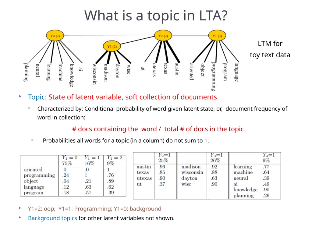
slide16. Topic: State of latent variable, soft collection of documents
Characterized by: Conditional probability of word given latent state, or, document frequency of word in collection:
# docs containing the word / total # of docs in the topic
Probabilities all words for a topic (in a column) do not sum to 1.

Y1=2: oop; Y1=1: Programming; Y1=0: background
Background topics for other latent variables not shown. What is a topic in LTA? LTM for
toy text data<br>
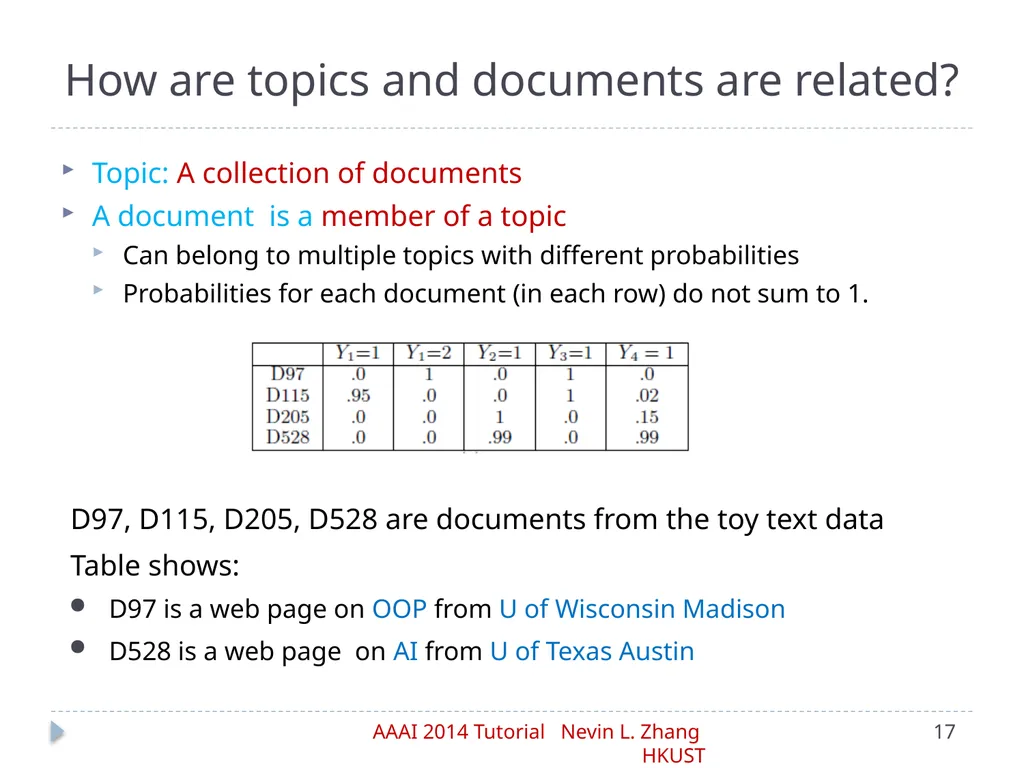
slide17. Topic: A collection of documents
A document is a member of a topic
Can belong to multiple topics with different probabilities
Probabilities for each document (in each row) do not sum to 1. How are topics and documents are related? D97, D115, D205, D528 are documents from the toy text data
Table shows:
D97 is a web page on OOP from U of Wisconsin Madison
D528 is a web page on AI from U of Texas Austin<br>
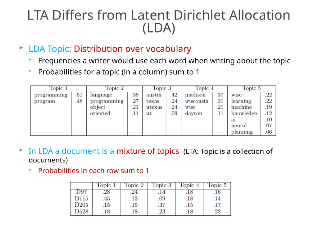
slide18. LDA Topic: Distribution over vocabulary
Frequencies a writer would use each word when writing about the topic
Probabilities for a topic (in a column) sum to 1

In LDA a document is a mixture of topics (LTA: Topic is a collection of documents)
Probabilities in each row sum to 1 LTA Differs from Latent Dirichlet Allocation (LDA)<br>
slide19. Basics

Aggregation of miniature topics

Topic extraction and characterization

Empirical results Latent Tree Models for Topic Detection<br>
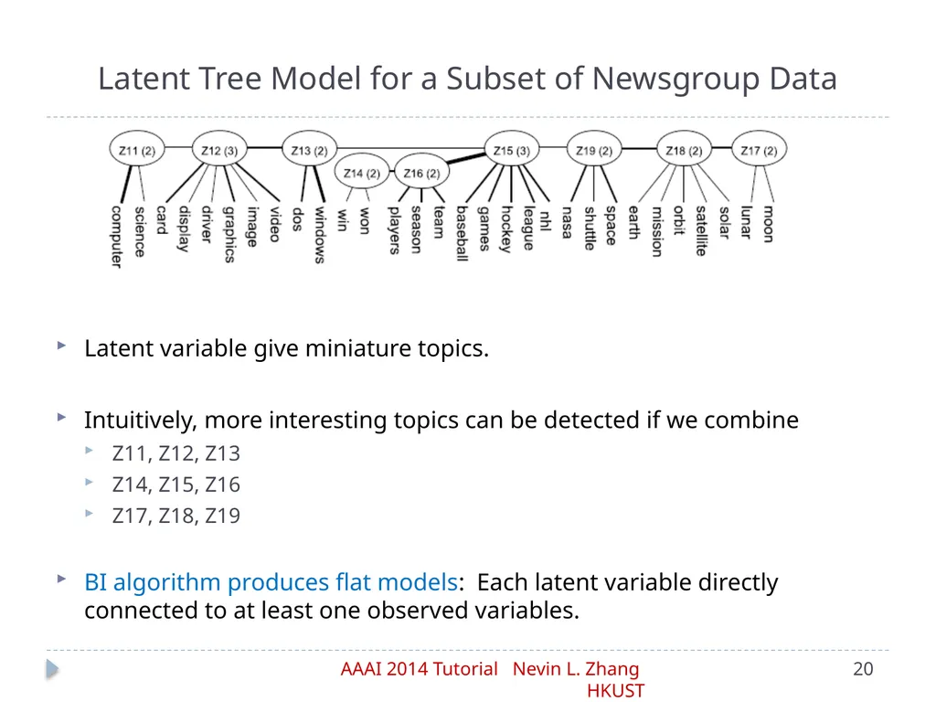
slide20. Latent variable give miniature topics.

Intuitively, more interesting topics can be detected if we combine
Z11, Z12, Z13
Z14, Z15, Z16
Z17, Z18, Z19

BI algorithm produces flat models: Each latent variable directly connected to at least one observed variables. Latent Tree Model for a Subset of Newsgroup Data<br>
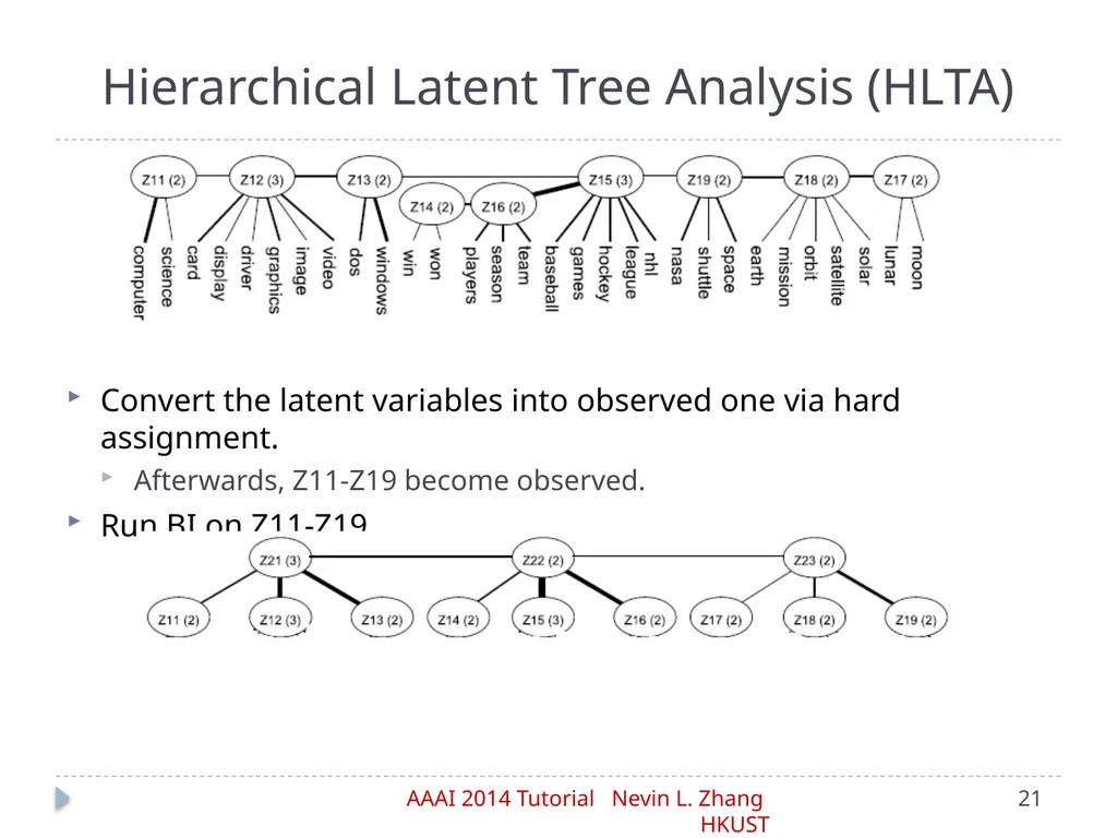
slide21. Convert the latent variables into observed one via hard assignment.
Afterwards, Z11-Z19 become observed.
Run BI on Z11-Z19 Hierarchical Latent Tree Analysis (HLTA)<br>
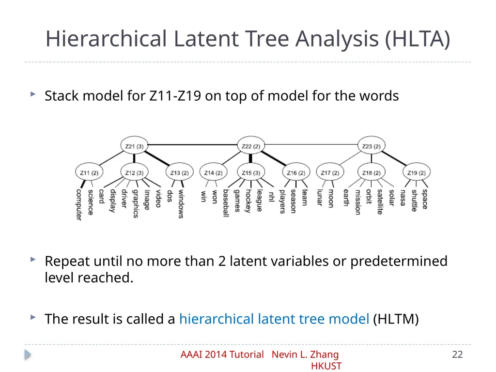
slide22. Stack model for Z11-Z19 on top of model for the words

Repeat until no more than 2 latent variables or predetermined level reached.

The result is called a hierarchical latent tree model (HLTM) Hierarchical Latent Tree Analysis (HLTA)<br>
slide23. Part II: Cannot determine edge orientations based solely on data.

Here hierarchical structure introduced to improve model interpretability.

Data + interpretability  hierarchical structure.

It does not necessarily improve model fit. Hierarchical Latent Tree Analysis (HLTA)<br>
slide24. Basics

Aggregation of miniature topics

Topic extraction and characterization

Empirical results Latent Tree Models for Topic Detection<br>
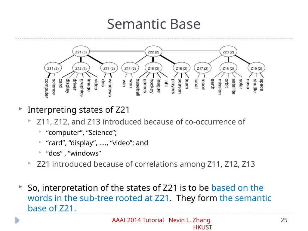
slide25. Interpreting states of Z21
Z11, Z12, and Z13 introduced because of co-occurrence of
“computer”, “Science”;
“card”, “display”, …., “video”; and
“dos” , “windows”
Z21 introduced because of correlations among Z11, Z12, Z13

So, interpretation of the states of Z21 is to be based on the words in the sub-tree rooted at Z21. They form the semantic base of Z21. Semantic Base<br>
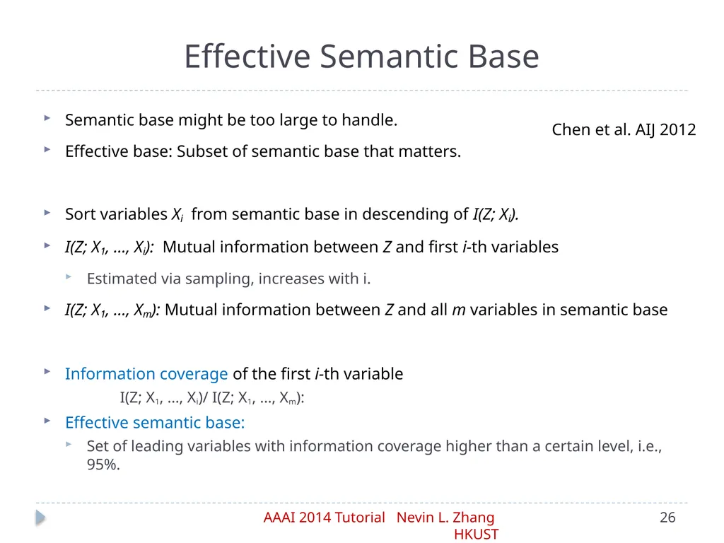
slide26. Semantic base might be too large to handle.
Effective base: Subset of semantic base that matters.

Sort variables Xi from semantic base in descending of I(Z; Xi).
I(Z; X1, …, Xi): Mutual information between Z and first i-th variables
Estimated via sampling, increases with i.
I(Z; X1, …, Xm): Mutual information between Z and all m variables in semantic base

Information coverage of the first i-th variable
I(Z; X1, …, Xi)/ I(Z; X1, …, Xm):
Effective semantic base:
Set of leading variables with information coverage higher than a certain level, i.e., 95%. Effective Semantic Base Chen et al. AIJ 2012<br>
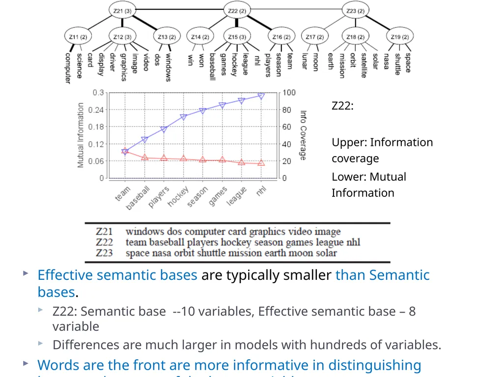
slide27. Effective semantic bases are typically smaller than Semantic bases.
Z22: Semantic base --10 variables, Effective semantic base – 8 variable
Differences are much larger in models with hundreds of variables.
Words are the front are more informative in distinguishing between the states of the latent variable. Z22:

Upper: Information coverage
Lower: Mutual Information<br>
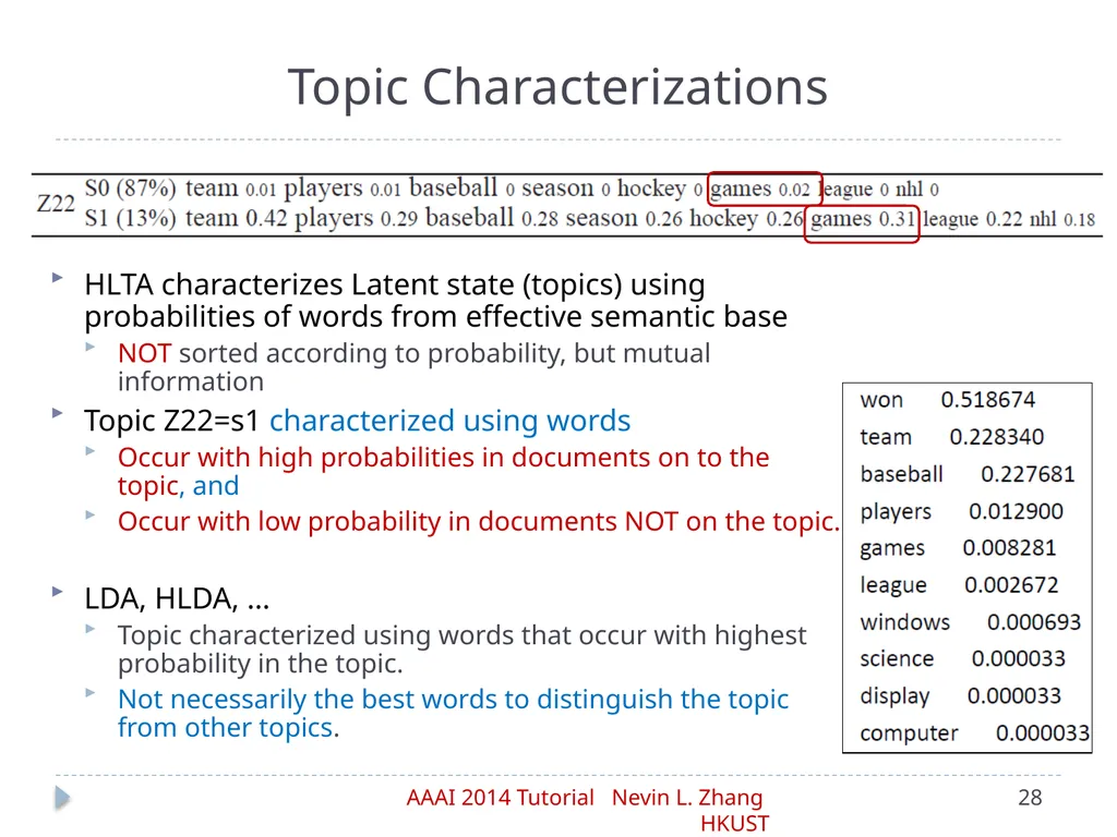
slide28. HLTA characterizes Latent state (topics) using probabilities of words from effective semantic base
NOT sorted according to probability, but mutual information
Topic Z22=s1 characterized using words
Occur with high probabilities in documents on to the topic, and
Occur with low probability in documents NOT on the topic.

LDA, HLDA, …
Topic characterized using words that occur with highest probability in the topic.
Not necessarily the best words to distinguish the topic from other topics. Topic Characterizations<br>
slide29. Basics

Aggregation of miniature topics

Topic extraction and characterization

Empirical results Latent Tree Models for Topic Detection<br>
slide30. Show the results of HLTA on real-world data

Compare HLTA with HLDA and LDA Empirical Results<br>
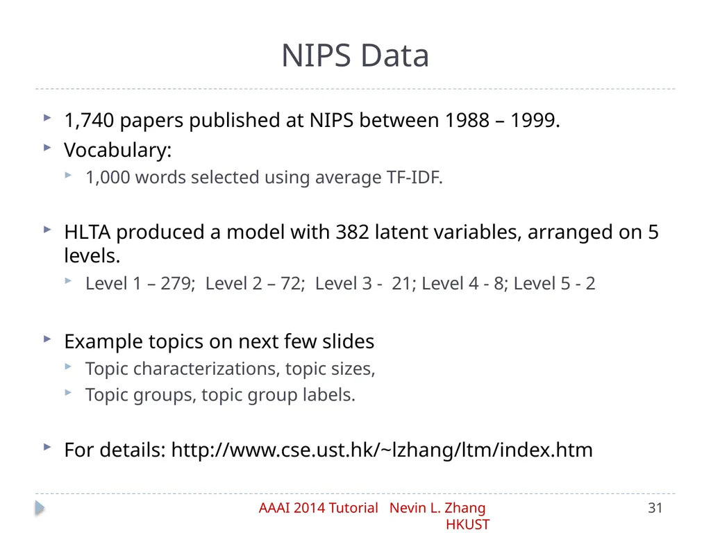
slide31. 1,740 papers published at NIPS between 1988 – 1999.
Vocabulary:
1,000 words selected using average TF-IDF.

HLTA produced a model with 382 latent variables, arranged on 5 levels.
Level 1 – 279; Level 2 – 72; Level 3 - 21; Level 4 - 8; Level 5 - 2

Example topics on next few slides
Topic characterizations, topic sizes,
Topic groups, topic group labels.

For details: http://www.cse.ust.hk/~lzhang/ltm/index.htm NIPS Data<br>
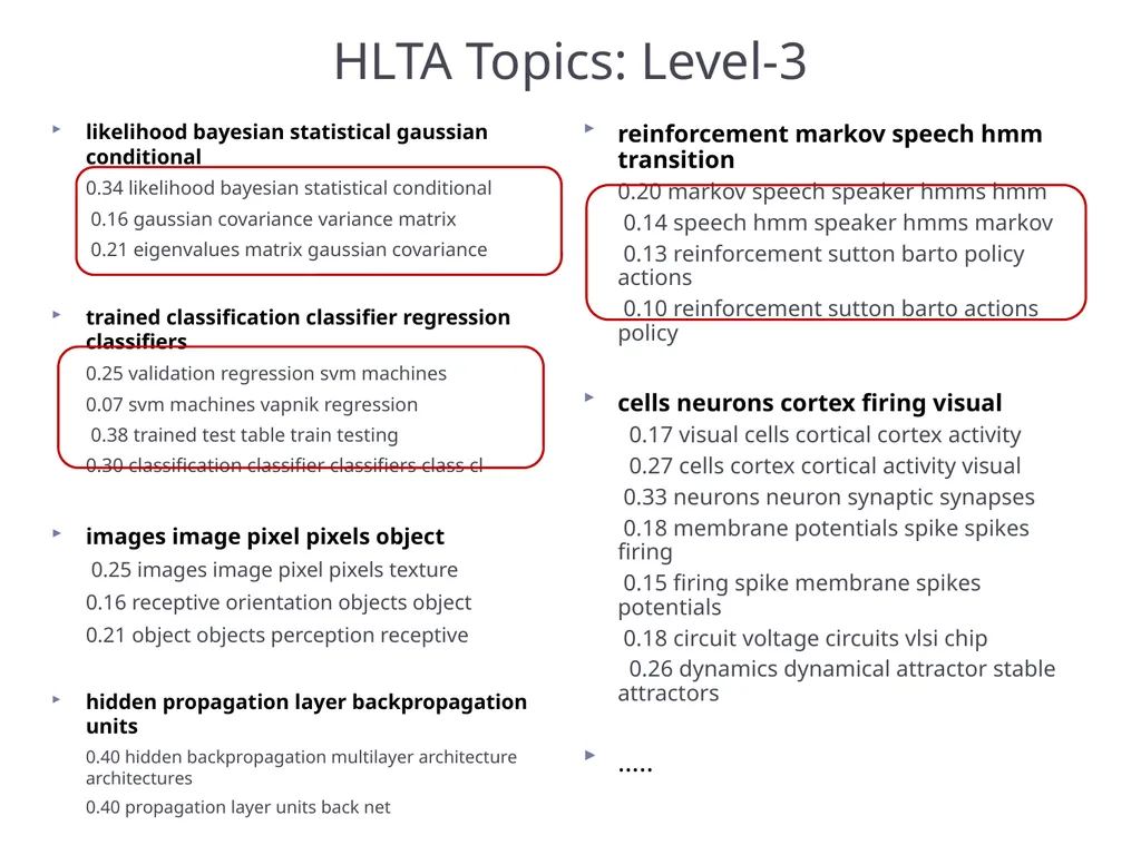
slide32. likelihood bayesian statistical gaussian conditional
0.34 likelihood bayesian statistical conditional
0.16 gaussian covariance variance matrix
0.21 eigenvalues matrix gaussian covariance

trained classification classifier regression classifiers
0.25 validation regression svm machines
0.07 svm machines vapnik regression
0.38 trained test table train testing
0.30 classification classifier classifiers class cl

images image pixel pixels object
0.25 images image pixel pixels texture
0.16 receptive orientation objects object
0.21 object objects perception receptive

hidden propagation layer backpropagation units
0.40 hidden backpropagation multilayer architecture architectures
0.40 propagation layer units back net HLTA Topics: Level-3 reinforcement markov speech hmm transition
0.20 markov speech speaker hmms hmm
0.14 speech hmm speaker hmms markov
0.13 reinforcement sutton barto policy actions
0.10 reinforcement sutton barto actions policy

cells neurons cortex firing visual
  0.17 visual cells cortical cortex activity
0.27 cells cortex cortical activity visual
0.33 neurons neuron synaptic synapses
0.18 membrane potentials spike spikes firing
0.15 firing spike membrane spikes potentials
0.18 circuit voltage circuits vlsi chip
  0.26 dynamics dynamical attractor stable attractors

…..<br>
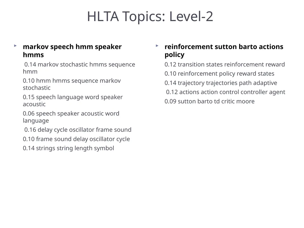
slide33. markov speech hmm speaker hmms
0.14 markov stochastic hmms sequence hmm
0.10 hmm hmms sequence markov stochastic
0.15 speech language word speaker acoustic
0.06 speech speaker acoustic word language
0.16 delay cycle oscillator frame sound
0.10 frame sound delay oscillator cycle
0.14 strings string length symbol HLTA Topics: Level-2 reinforcement sutton barto actions policy
0.12 transition states reinforcement reward
0.10 reinforcement policy reward states
0.14 trajectory trajectories path adaptive
0.12 actions action control controller agent
0.09 sutton barto td critic moore<br>
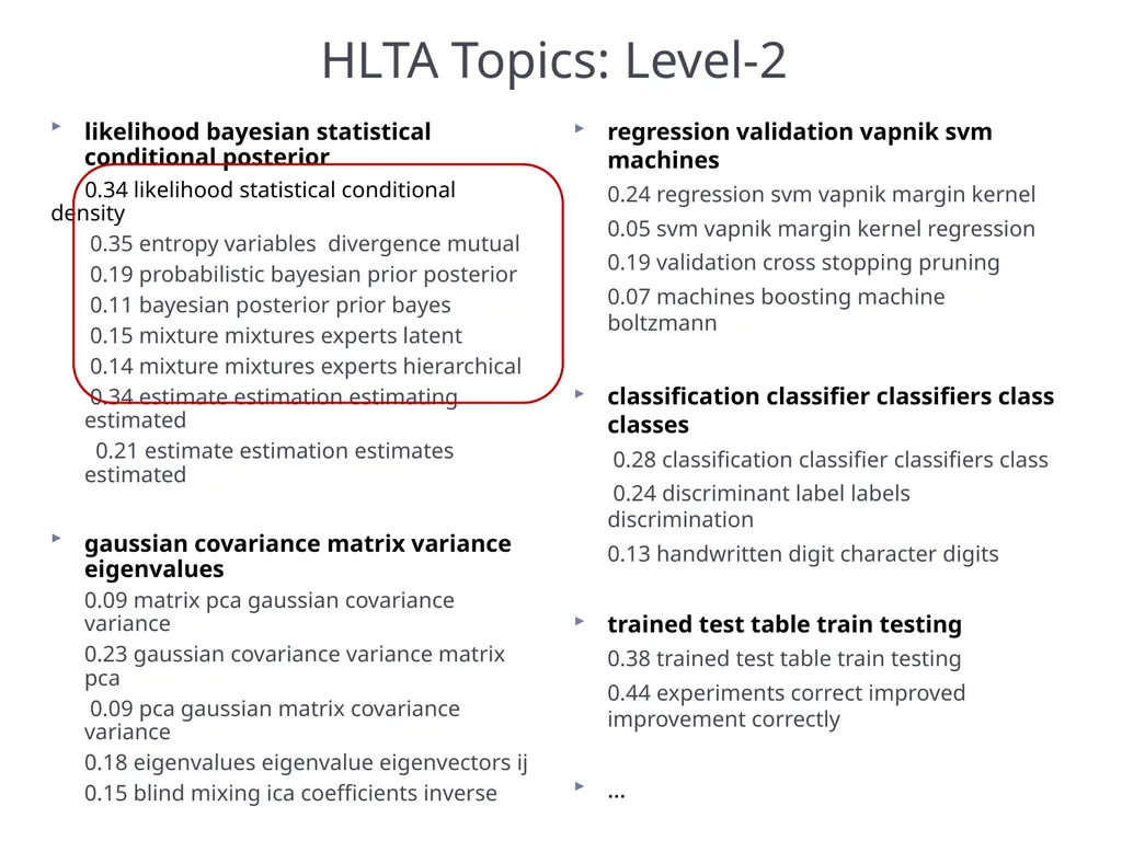
slide34. likelihood bayesian statistical conditional posterior
0.34 likelihood statistical conditional density
0.35 entropy variables divergence mutual
0.19 probabilistic bayesian prior posterior
0.11 bayesian posterior prior bayes
0.15 mixture mixtures experts latent
0.14 mixture mixtures experts hierarchical
0.34 estimate estimation estimating estimated
  0.21 estimate estimation estimates estimated

gaussian covariance matrix variance eigenvalues
0.09 matrix pca gaussian covariance variance
0.23 gaussian covariance variance matrix pca
0.09 pca gaussian matrix covariance variance
0.18 eigenvalues eigenvalue eigenvectors ij
0.15 blind mixing ica coefficients inverse HLTA Topics: Level-2 regression validation vapnik svm machines
0.24 regression svm vapnik margin kernel
0.05 svm vapnik margin kernel regression
0.19 validation cross stopping pruning
0.07 machines boosting machine boltzmann

classification classifier classifiers class classes
0.28 classification classifier classifiers class
0.24 discriminant label labels discrimination
0.13 handwritten digit character digits

trained test table train testing
0.38 trained test table train testing
0.44 experiments correct improved improvement correctly

…<br>
slide35. likelihood statistical conditional density log
0.30 likelihood conditional log em maximum
0.42 statistical statistics
0.19 density densities

entropy variables variable divergence mutual
0.16 entropy divergence mutual
0.31 variables variable

bayesian posterior probabilistic prior bayes
0.19 bayesian prior bayes posterior priors
0.09 bayesian posterior prior priors bayes
0.29 probabilistic distributions probabilities
0.16 inference gibbs sampling generative
0.19 mackay independent averaging ensemble
0.08 belief graphical variational
0.09 monte carlo
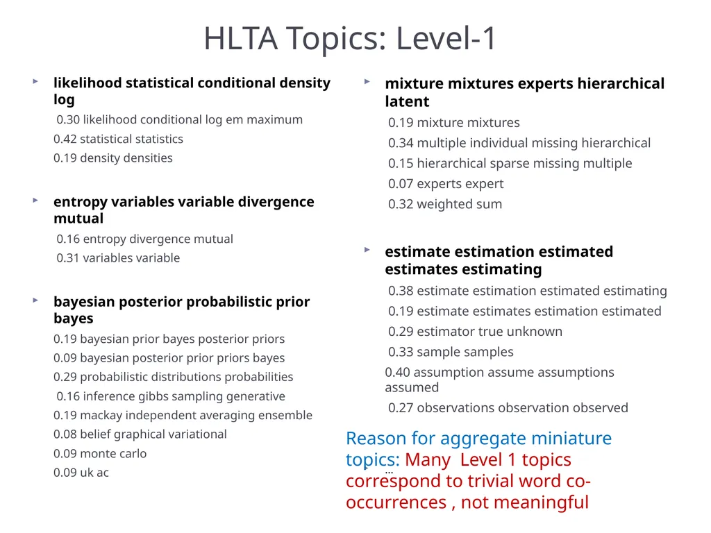
0.09 uk ac HLTA Topics: Level-1 mixture mixtures experts hierarchical latent
0.19 mixture mixtures
0.34 multiple individual missing hierarchical
0.15 hierarchical sparse missing multiple
0.07 experts expert
0.32 weighted sum

estimate estimation estimated estimates estimating
 0.38 estimate estimation estimated estimating
0.19 estimate estimates estimation estimated
0.29 estimator true unknown
0.33 sample samples
0.40 assumption assume assumptions assumed
0.27 observations observation observed

… Reason for aggregate miniature topics: Many Level 1 topics correspond to trivial word co-occurrences , not meaningful<br>
slide36. Level 5
visual cortex cells neurons firing
0.37 visual cortex firing neurons cells
0.39 visual cells firing cortex neurons
0.25 images image pixel hidden trained
0.09 hidden trained images image pixel
0.20 trained hidden images image pixel
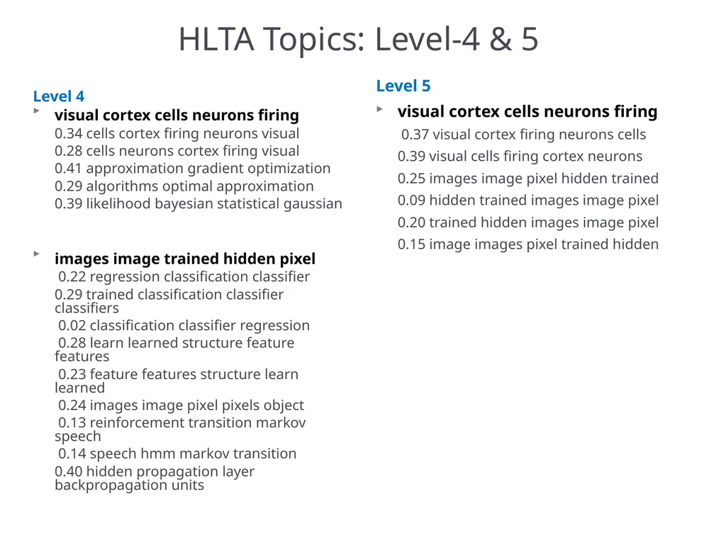
0.15 image images pixel trained hidden HLTA Topics: Level-4 & 5 Level 4
visual cortex cells neurons firing
0.34 cells cortex firing neurons visual
0.28 cells neurons cortex firing visual
0.41 approximation gradient optimization
0.29 algorithms optimal approximation
0.39 likelihood bayesian statistical gaussian

images image trained hidden pixel
0.22 regression classification classifier
0.29 trained classification classifier classifiers
0.02 classification classifier regression
0.28 learn learned structure feature features
0.23 feature features structure learn learned
0.24 images image pixel pixels object
0.13 reinforcement transition markov speech
0.14 speech hmm markov transition
0.40 hidden propagation layer backpropagation units<br>
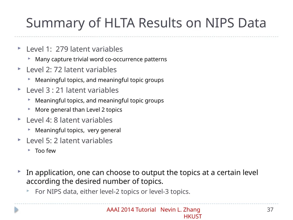
slide37. Level 1: 279 latent variables
Many capture trivial word co-occurrence patterns
Level 2: 72 latent variables
Meaningful topics, and meaningful topic groups
Level 3 : 21 latent variables
Meaningful topics, and meaningful topic groups
More general than Level 2 topics
Level 4: 8 latent variables
Meaningful topics, very general
Level 5: 2 latent variables
Too few

In application, one can choose to output the topics at a certain level according the desired number of topics.
For NIPS data, either level-2 topics or level-3 topics. Summary of HLTA Results on NIPS Data<br>
slide38. units hidden layer unit weight
gaussian log density likelihood estimate
margin kernel support xi bound
generalization student weight teacher optimal
gaussian bayesian kernel evidence posterior
chip analog circuit neuron voltage
classifier rbf class classifiers classification
speech recognition hmm context word
ica independent separation source sources
image images matching level object
tree trees node nodes boosting
variables variable bayesian conditional
family face strategy differential functional
weighting source grammar sequences
polynomial regression derivative
em machine annealing max min

regression prediction selection criterion query
validation obs generalization cross pruning
mlp risk classifier classification confidence
loss song transfer bounds wt
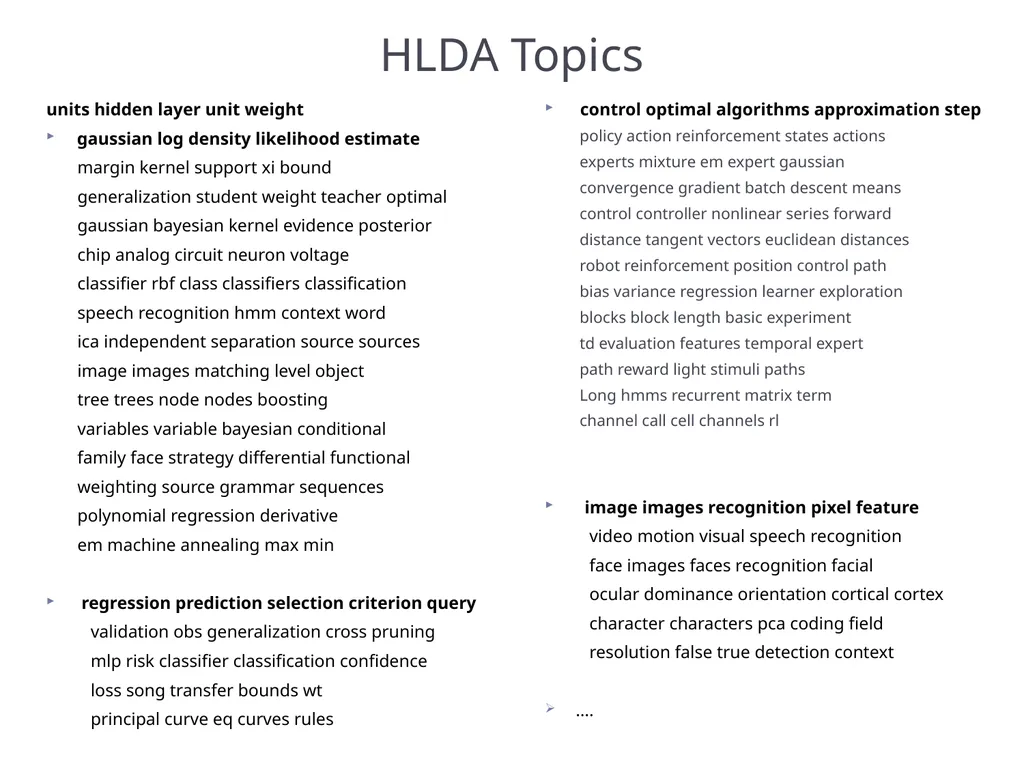
principal curve eq curves rules HLDA Topics control optimal algorithms approximation step
policy action reinforcement states actions
experts mixture em expert gaussian
convergence gradient batch descent means
control controller nonlinear series forward
distance tangent vectors euclidean distances
robot reinforcement position control path
bias variance regression learner exploration
blocks block length basic experiment
td evaluation features temporal expert
path reward light stimuli paths
Long hmms recurrent matrix term
channel call cell channels rl

image images recognition pixel feature
video motion visual speech recognition
face images faces recognition facial
ocular dominance orientation cortical cortex
character characters pca coding field
resolution false true detection context

….<br>
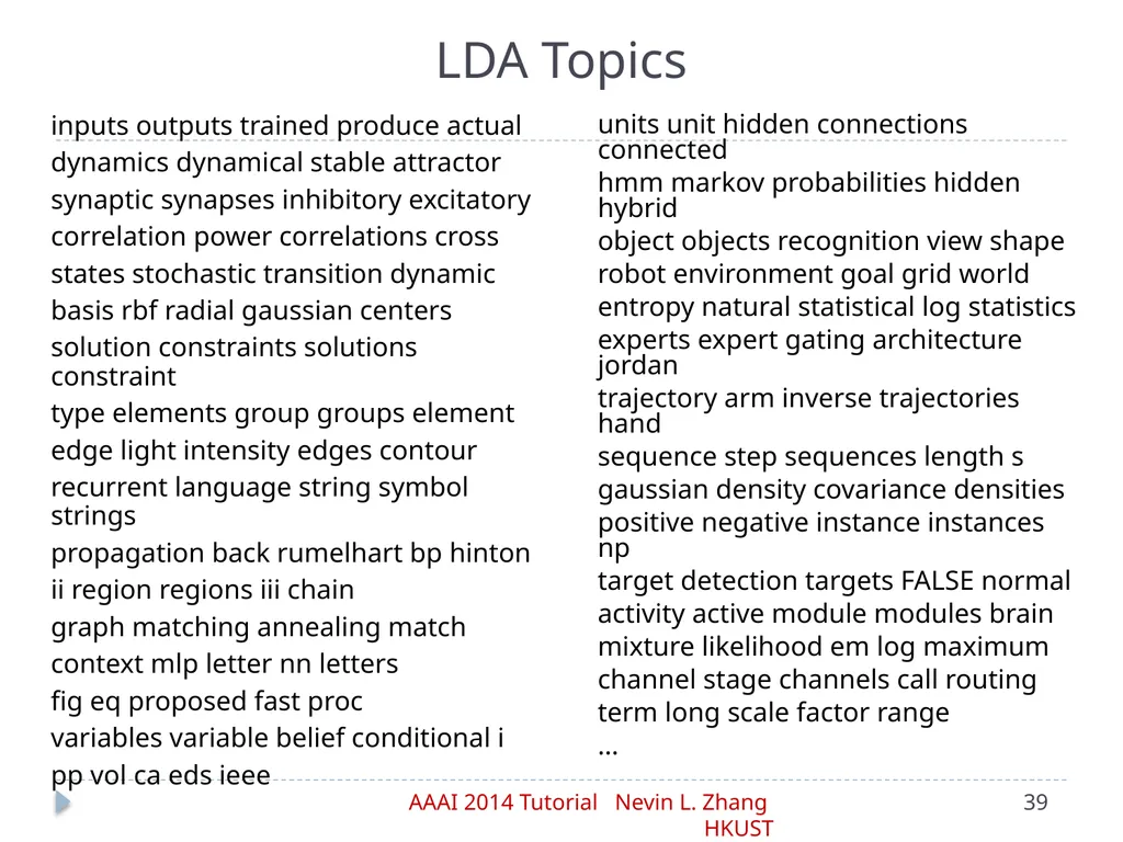
slide39. inputs outputs trained produce actual
dynamics dynamical stable attractor
synaptic synapses inhibitory excitatory
correlation power correlations cross
states stochastic transition dynamic
basis rbf radial gaussian centers
solution constraints solutions constraint
type elements group groups element
edge light intensity edges contour
recurrent language string symbol strings
propagation back rumelhart bp hinton
ii region regions iii chain
graph matching annealing match
context mlp letter nn letters
fig eq proposed fast proc
variables variable belief conditional i
pp vol ca eds ieee LDA Topics units unit hidden connections connected
hmm markov probabilities hidden hybrid
object objects recognition view shape
robot environment goal grid world
entropy natural statistical log statistics
experts expert gating architecture jordan
trajectory arm inverse trajectories hand
sequence step sequences length s
gaussian density covariance densities
positive negative instance instances np
target detection targets FALSE normal
activity active module modules brain
mixture likelihood em log maximum
channel stage channels call routing
term long scale factor range
…<br>
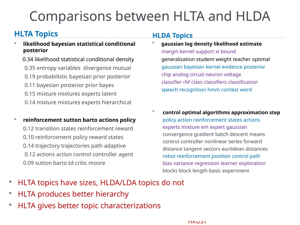
slide40. HLTA Topics
likelihood bayesian statistical conditional posterior
0.34 likelihood statistical conditional density
0.35 entropy variables divergence mutual
0.19 probabilistic bayesian prior posterior
0.11 bayesian posterior prior bayes
0.15 mixture mixtures experts latent
0.14 mixture mixtures experts hierarchical

reinforcement sutton barto actions policy
0.12 transition states reinforcement reward
0.10 reinforcement policy reward states
0.14 trajectory trajectories path adaptive
0.12 actions action control controller agent
0.09 sutton barto td critic moore Comparisons between HLTA and HLDA HLDA Topics
gaussian log density likelihood estimate
margin kernel support xi bound
generalization student weight teacher optimal
gaussian bayesian kernel evidence posterior
chip analog circuit neuron voltage
classifier rbf class classifiers classification
speech recognition hmm context word


control optimal algorithms approximation step
policy action reinforcement states actions
experts mixture em expert gaussian
convergence gradient batch descent means
control controller nonlinear series forward
distance tangent vectors euclidean distances
robot reinforcement position control path
bias variance regression learner exploration
blocks block length basic experiment HLTA topics have sizes, HLDA/LDA topics do not
HLTA produces better hierarchy
HLTA gives better topic characterizations<br>
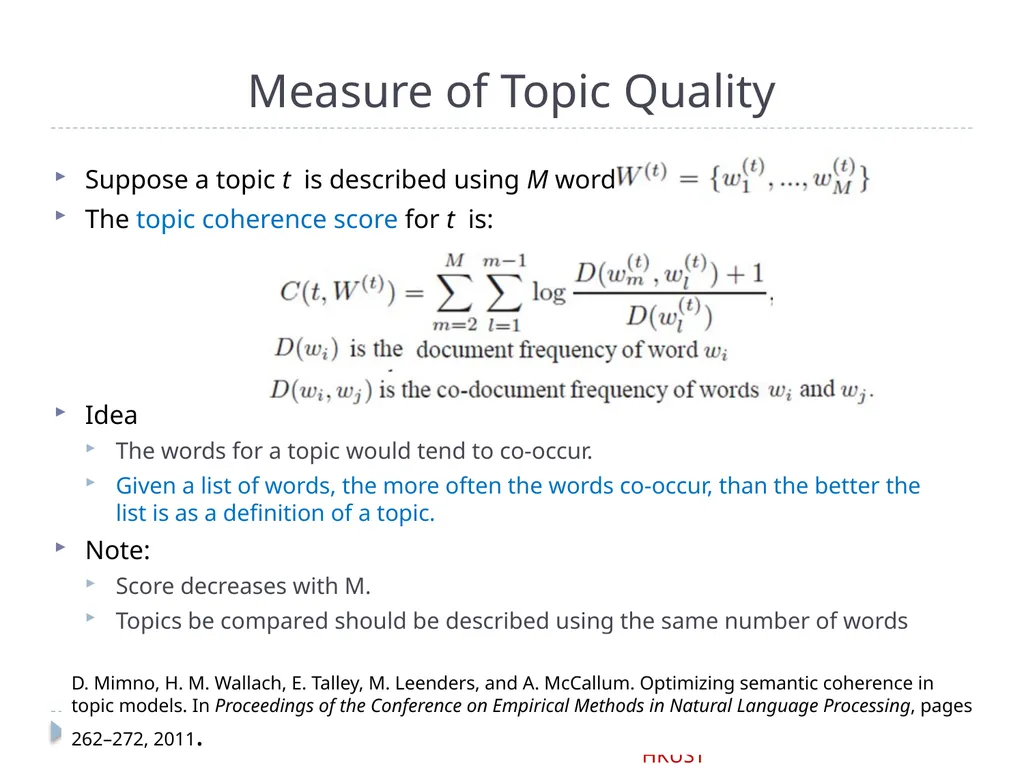
slide41. Suppose a topic t is described using M words
The topic coherence score for t is:

Idea
The words for a topic would tend to co-occur.
Given a list of words, the more often the words co-occur, than the better the list is as a definition of a topic.
Note:
Score decreases with M.
Topics be compared should be described using the same number of words Measure of Topic Quality D. Mimno, H. M. Wallach, E. Talley, M. Leenders, and A. McCallum. Optimizing semantic coherence in topic models. In Proceedings of the Conference on Empirical Methods in Natural Language Processing, pages 262–272, 2011.<br>
slide42. HLTA (L3-L4): All non-background topics from Levels 3 and 4: 47
HLTA (L2-L3-L4): All non-background topics from Levels 2, 3 and 4: 140

LDA was instructed to find two sets of topics with 47 and140 topics

HLDA found more 179.
HLDA-s: A subset of the HLDA topics were sampled for fair comparison. HLTA Found More Coherent Topics than LDA and HLDA<br>
slide43. Regard LDA, HLDA and HLTA as methods for text modeling
Build a probabilistic model for the corpus

Evaluation:
Per-document held-out loglikelihood (-log(perplexity)).
Measure performance of model on predicting unseen data

Data:
NIPS: 1,740 papers from NIPS, 1,000 words,
JACM: 536 abstracts from J of ACM, 1,809 words.
NEWSGROUP: 20,000 newsgroup posts, 1,000 words. Comparisons in Terms of Model Fit<br>
slide44. HLTA results robust w.r.t UD-test threshold
The values 1, 3, 5 are from literature on Bayes factor (see Part III)

LDA produced by far worst models in all cases.
HLTA out-performed HLDA on NIPS, tied on JACP, and beaten on Newsgroup
Caution: Better model does not implies better topics

Running time on NIPS:
LDA – 3.6 hours, HLTA – 17 hours, HLDA – 68 hours.<br>
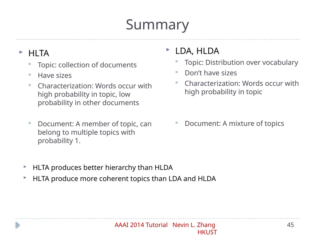
slide45. HLTA
Topic: collection of documents
Have sizes
Characterization: Words occur with high probability in topic, low probability in other documents

Document: A member of topic, can belong to multiple topics with probability 1. Summary LDA, HLDA
Topic: Distribution over vocabulary
Don’t have sizes
Characterization: Words occur with high probability in topic

Document: A mixture of topics HLTA produces better hierarchy than HLDA
HLTA produce more coherent topics than LDA and HLDA<br>
slide46. Part III: Applications Approximate Inference in Bayesian networks

Analysis of social survey data

Topic detection

Analysis of medical symptom survey data

Software<br>
slide47. Background of Research Common practice in China, increasingly in Western world
Patients of a WM disease divided into several TCM classes
Different classes are treated differently using TCM treatments.

Example:
WM disease: Depression
TCM Classes:
Liver-Qi Stagnation (肝气郁结). Treatment principle: 疏肝解郁， Prescription: 柴胡疏肝散
Deficiency of Liver Yin and Kidney Yin (肝肾阴虚)：Treatment principle: 滋肾养肝， Prescription: 逍遥散合六味地黄丸
Vacuity of both heart and spleen (心脾两虚). Treatment principle: 益气健脾, Prescription: 归脾汤
…. Page 47<br>
slide48. Key Question How should patients of a WM disease be divided into subclasses from the TCM perspective?
What TCM classes?
What are the characteristics of each TCM class?
How to differentiate different TCM classes?

Important for
Clinic practice
Research
Randomized controlled trials for efficacy
Modern biomedical understanding of TCM concepts

No consensus. Different doctors/researchers use different schemes. Key weakness of TCM. Page 48<br>
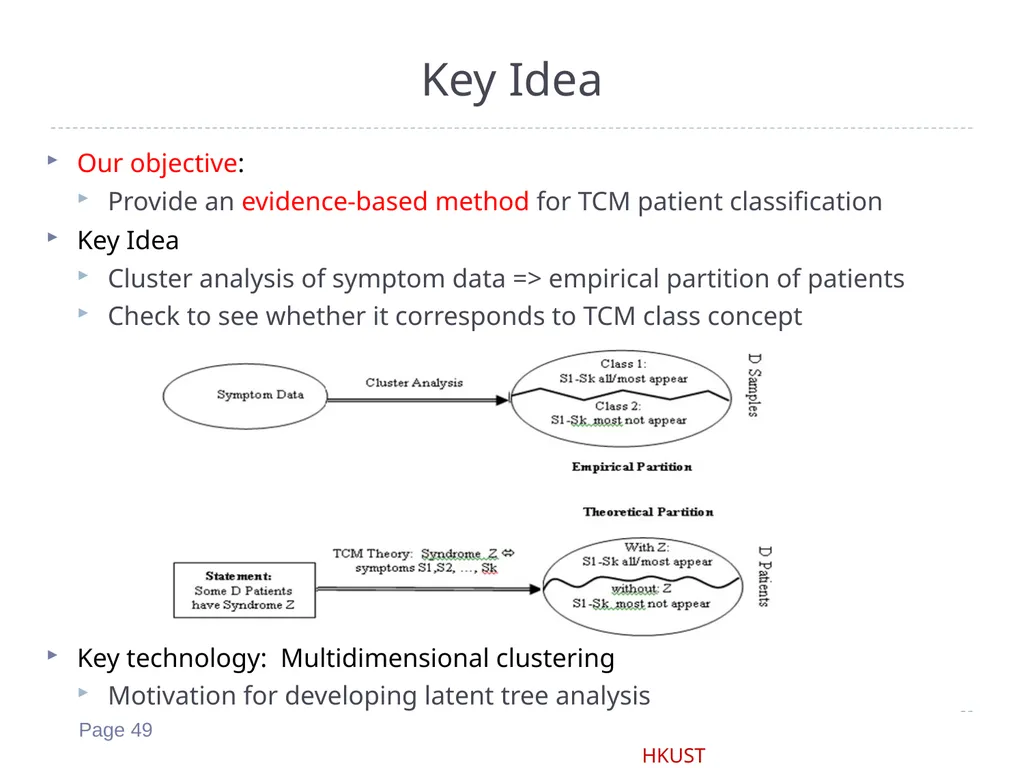
slide49. Key Idea Our objective:
Provide an evidence-based method for TCM patient classification
Key Idea
Cluster analysis of symptom data => empirical partition of patients
Check to see whether it corresponds to TCM class concept

Key technology: Multidimensional clustering
Motivation for developing latent tree analysis Page 49<br>
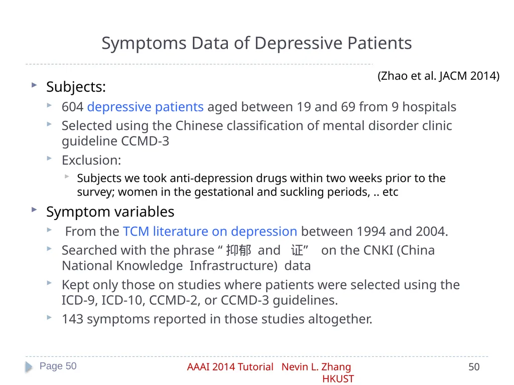
slide50. Symptoms Data of Depressive Patients Subjects:
604 depressive patients aged between 19 and 69 from 9 hospitals
Selected using the Chinese classification of mental disorder clinic guideline CCMD-3
Exclusion:
Subjects we took anti-depression drugs within two weeks prior to the survey; women in the gestational and suckling periods, .. etc
Symptom variables
From the TCM literature on depression between 1994 and 2004.
Searched with the phrase “抑郁 and 证” on the CNKI (China National Knowledge Infrastructure) data
Kept only those on studies where patients were selected using the ICD-9, ICD-10, CCMD-2, or CCMD-3 guidelines.
143 symptoms reported in those studies altogether. Page 50 (Zhao et al. JACM 2014)<br>
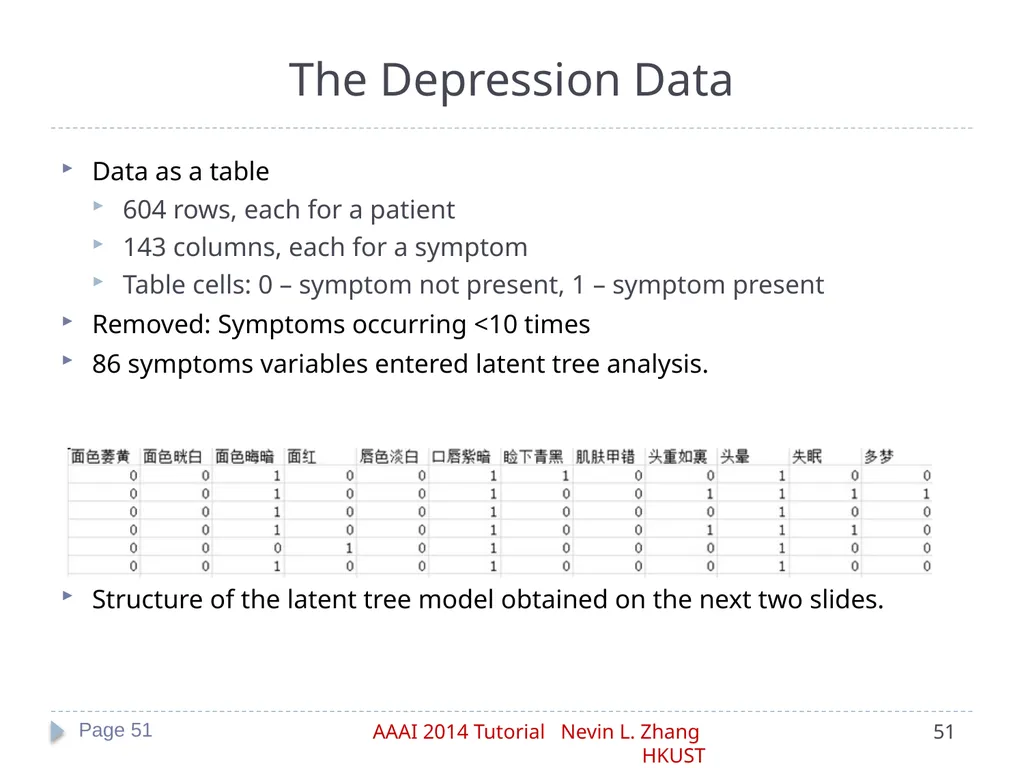
slide51. The Depression Data Data as a table
604 rows, each for a patient
143 columns, each for a symptom
Table cells: 0 – symptom not present, 1 – symptom present
Removed: Symptoms occurring <10 times
86 symptoms variables entered latent tree analysis.

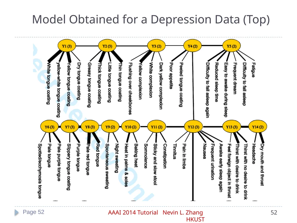
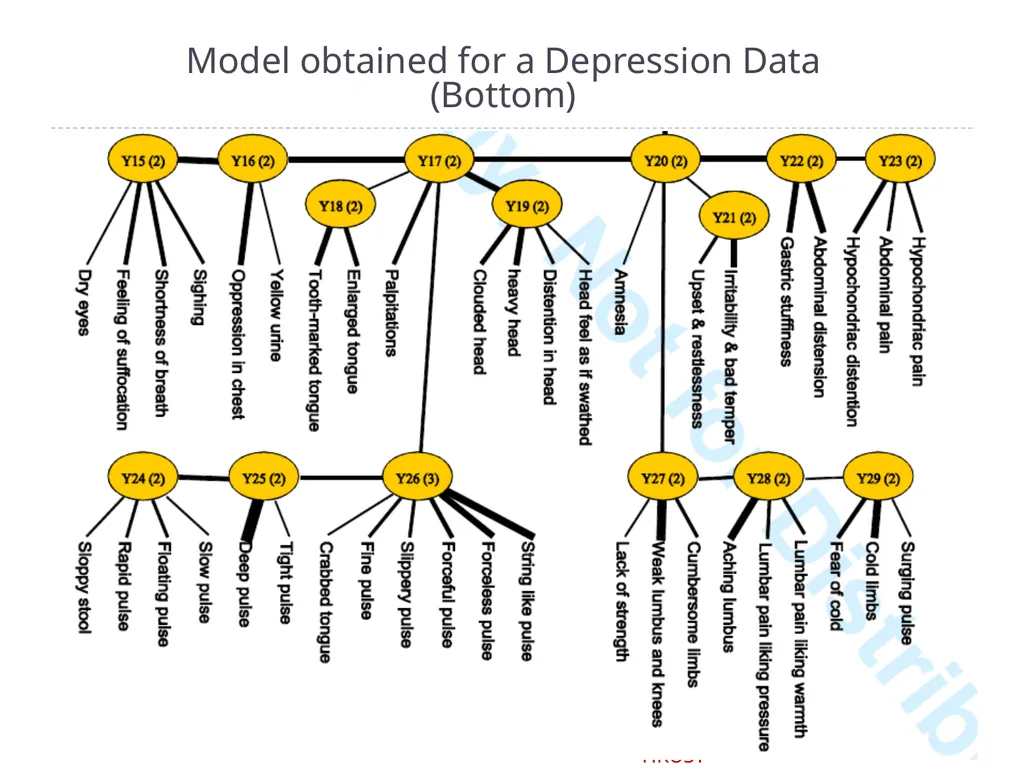
Structure of the latent tree model obtained on the next two slides. Page 51<br>
slide52. Model Obtained for a Depression Data (Top) Page 52<br>
slide53. Model obtained for a Depression Data (Bottom) Page 53<br>
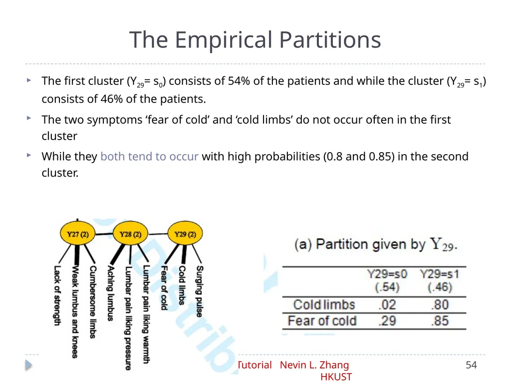
slide54. The Empirical Partitions Page 54 The first cluster (Y29= s0) consists of 54% of the patients and while the cluster (Y29= s1) consists of 46% of the patients.
The two symptoms ‘fear of cold’ and ‘cold limbs’ do not occur often in the first cluster
While they both tend to occur with high probabilities (0.8 and 0.85) in the second cluster.<br>
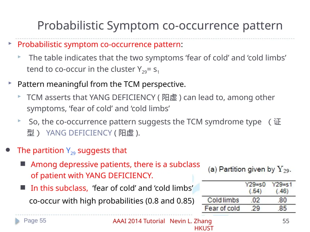
slide55. Probabilistic Symptom co-occurrence pattern Probabilistic symptom co-occurrence pattern:
The table indicates that the two symptoms ‘fear of cold’ and ‘cold limbs’ tend to co-occur in the cluster Y29= s1
Pattern meaningful from the TCM perspective.
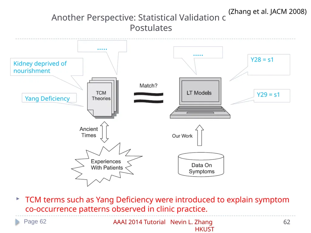
TCM asserts that YANG DEFICIENCY (阳虚) can lead to, among other symptoms, ‘fear of cold’ and ‘cold limbs’
So, the co-occurrence pattern suggests the TCM symdrome type （证型） YANG DEFICIENCY (阳虚). Page 55 The partition Y29 suggests that
Among depressive patients, there is a subclass of patient with YANG DEFICIENCY.
In this subclass, ‘fear of cold’ and ‘cold limbs’
co-occur with high probabilities (0.8 and 0.85)<br>
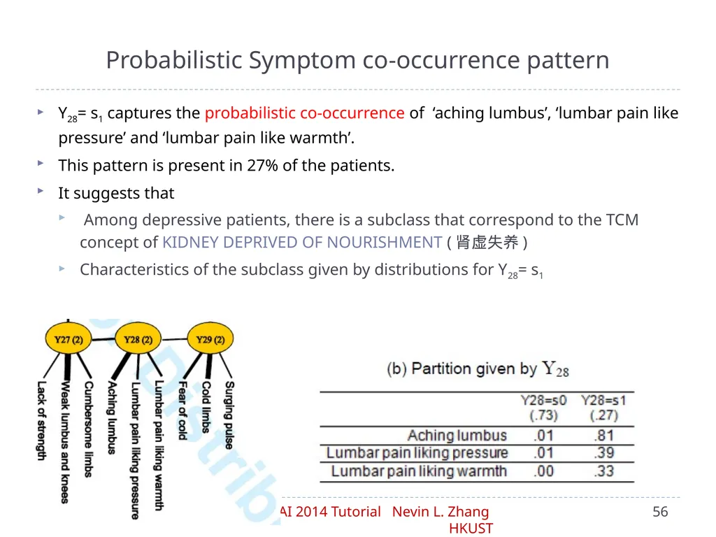
slide56. Probabilistic Symptom co-occurrence pattern Page 56 Y28= s1 captures the probabilistic co-occurrence of ‘aching lumbus’, ‘lumbar pain like pressure’ and ‘lumbar pain like warmth’.
This pattern is present in 27% of the patients.
It suggests that
Among depressive patients, there is a subclass that correspond to the TCM concept of KIDNEY DEPRIVED OF NOURISHMENT (肾虚失养)
Characteristics of the subclass given by distributions for Y28= s1<br>
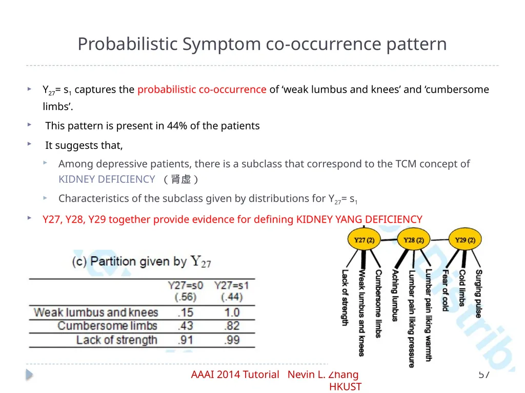
slide57. Probabilistic Symptom co-occurrence pattern Y27= s1 captures the probabilistic co-occurrence of ‘weak lumbus and knees’ and ‘cumbersome limbs’.
This pattern is present in 44% of the patients
It suggests that,
Among depressive patients, there is a subclass that correspond to the TCM concept of KIDNEY DEFICIENCY （肾虚）
Characteristics of the subclass given by distributions for Y27= s1
Y27, Y28, Y29 together provide evidence for defining KIDNEY YANG DEFICIENCY<br>
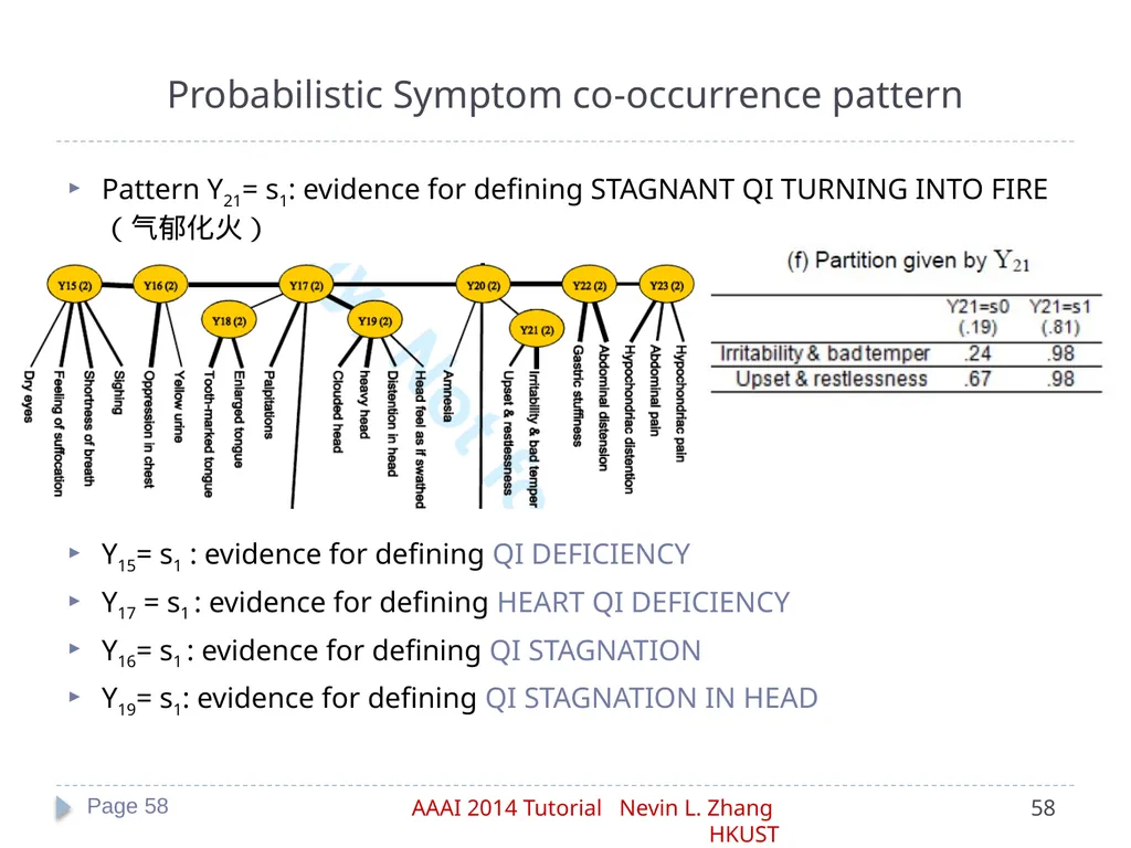
slide58. Probabilistic Symptom co-occurrence pattern Pattern Y21= s1: evidence for defining STAGNANT QI TURNING INTO FIRE （气郁化火）

Y15= s1 : evidence for defining QI DEFICIENCY
Y17 = s1 : evidence for defining HEART QI DEFICIENCY
Y16= s1 : evidence for defining QI STAGNATION
Y19= s1: evidence for defining QI STAGNATION IN HEAD Page 58<br>
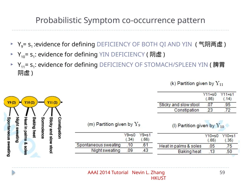
slide59. Probabilistic Symptom co-occurrence pattern Y9= s1 :evidence for defining DEFICIENCY OF BOTH QI AND YIN (气阴两虚)
Y10= s1: evidence for defining YIN DEFICIENCY (阴虚)
Y11= s1: evidence for defining DEFICIENCY OF STOMACH/SPLEEN YIN (脾胃阴虚) Page 59<br>
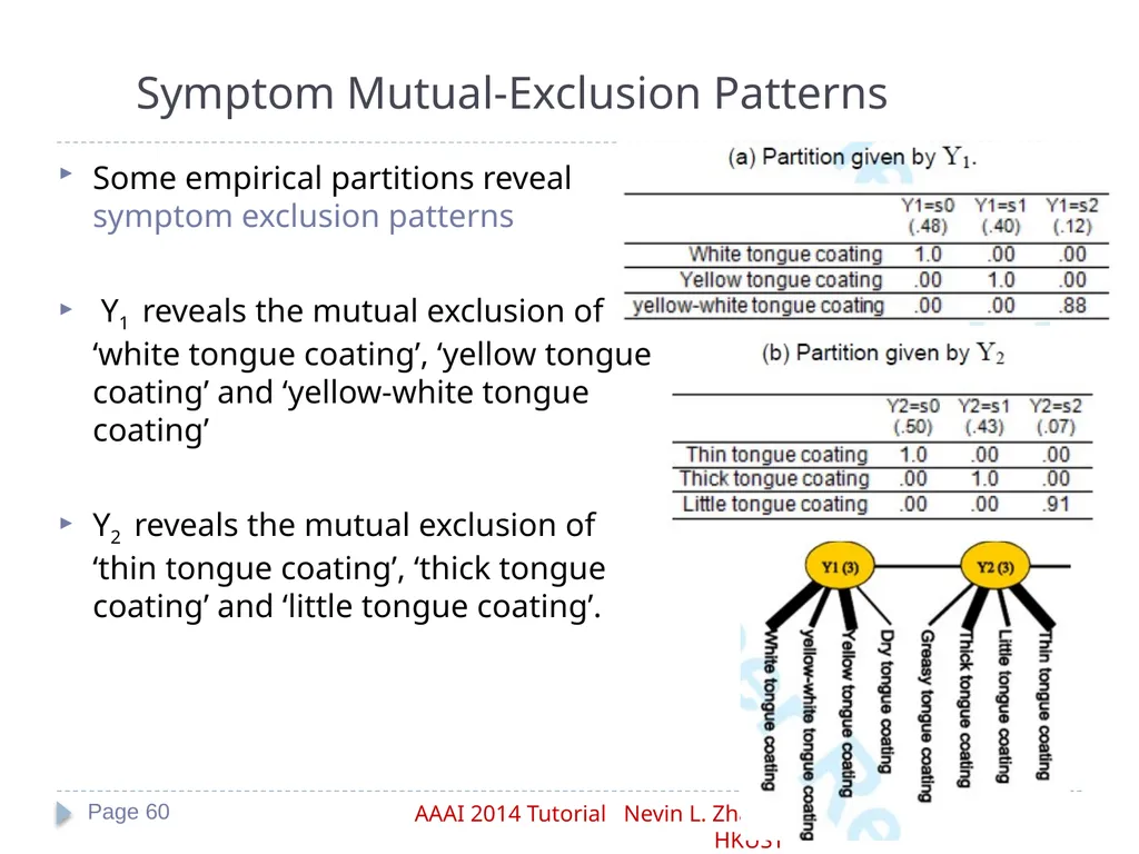
slide60. Symptom Mutual-Exclusion Patterns Some empirical partitions reveal symptom exclusion patterns

Y1 reveals the mutual exclusion of ‘white tongue coating’, ‘yellow tongue coating’ and ‘yellow-white tongue coating’

Y2 reveals the mutual exclusion of ‘thin tongue coating’, ‘thick tongue coating’ and ‘little tongue coating’. Page 60<br>
slide61. Summary of TCM Data Analysis By analyzing 604 cases of depressive patient data using latent tree models we have discovered a host of probabilistic symptom co-occurrence patterns and symptom mutual-exclusion patterns.

Most of the co-occurrence patterns have clear TCM syndrome connotations, while the mutual-exclusion patterns are also reasonable and meaningful.

The patterns can be used as evidence for the task of defining TCM classes in the context of depressive patients and for differentiating between those classes. Page 61<br>
slide62. Another Perspective: Statistical Validation of TCM Postulates Page 62 (Zhang et al. JACM 2008) Yang Deficiency Y29 = s1 Kidney deprived of nourishment Y28 = s1 TCM terms such as Yang Deficiency were introduced to explain symptom co-occurrence patterns observed in clinic practice. ….. …..<br>
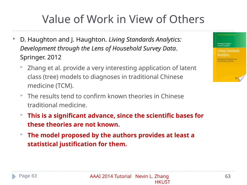
slide63. Value of Work in View of Others D. Haughton and J. Haughton. Living Standards Analytics: Development through the Lens of Household Survey Data. Springer. 2012
Zhang et al. provide a very interesting application of latent class (tree) models to diagnoses in traditional Chinese medicine (TCM).
The results tend to confirm known theories in Chinese traditional medicine.
This is a significant advance, since the scientific bases for these theories are not known.
The model proposed by the authors provides at least a statistical justification for them. Page 63<br>
slide64. Part III: Applications Approximate Inference in Bayesian networks

Analysis of social survey data

Topic detection

Analysis of medical symptom survey data

Software<br>
slide65. http://www.cse.ust.hk/faculty/lzhang/ltm/index.htm
Implementation of LTM learning algorithms: EAST, BI
Tool for manipulate LTMs: Lantern
LTM for topic detection: HLTA

Implementation of other LTM learning algorithms
BIN-A, BIN-G, CL and LCM:
http://people.kyb.tuebingen.mpg.de/harmeling/code/ltt-1.4.tar
CFHLC:
https://sites.google.com/site/raphaelmouradeng/home/programs
NJ, RG, CLRG and regCLRG:
http://people.csail.mit.edu/myungjin/latentTree.html
− NJ (fast implementation):
http://nimbletwist.com/software/ninja Software<br>