
Least-squares best-fitting polynomials



Description: Least-squares best-fitting polynomials Introduction In this topic, we will Describe approximating Au v when no exact solution exists Introduce the normal equation Use the normal equation to find the Best-fitting linear polynomial that
Related Topics
Download Presentation
"Least-squares best-fitting polynomials" is the property of its rightful owner. Permission is granted to download and print the materials on this website for personal, non-commercial use only, and to display it on your personal computer provided you do not modify the materials and that you retain all copyright notices contained in the materials. By downloading content from our website, you accept the terms of this agreement.
Presentation Transcript
slide1. Least-squares best-fitting polynomials<br>
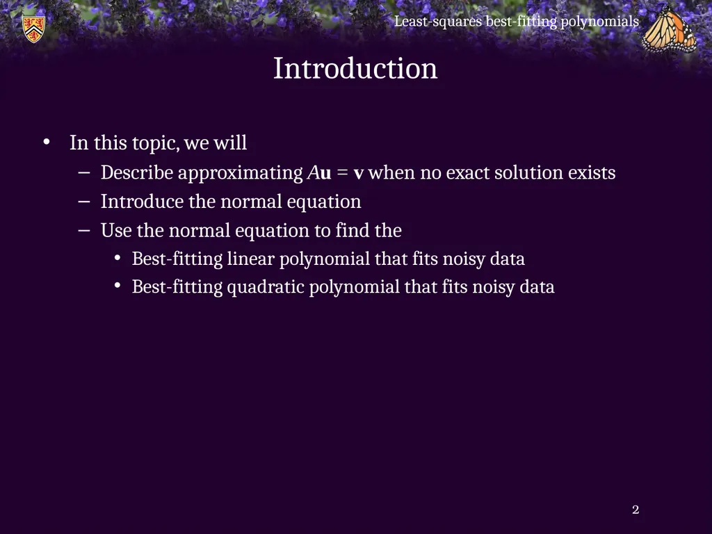
slide2. Introduction In this topic, we will
Describe approximating Au = v when no exact solution exists
Introduce the normal equation
Use the normal equation to find the
Best-fitting linear polynomial that fits noisy data
Best-fitting quadratic polynomial that fits noisy data Least-squares best-fitting polynomials 2<br>
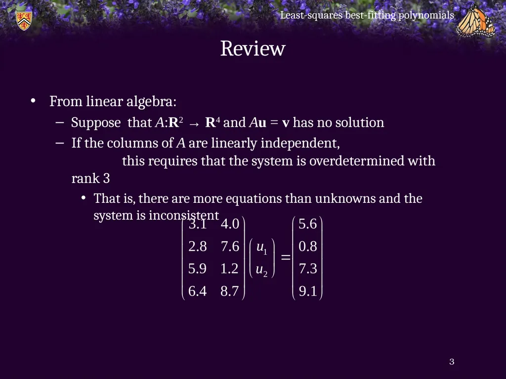
slide3. Review From linear algebra:
Suppose that A:R2 → R4 and Au = v has no solution
If the columns of A are linearly independent, this requires that the system is overdetermined with rank 3
That is, there are more equations than unknowns and the system is inconsistent Least-squares best-fitting polynomials 3<br>
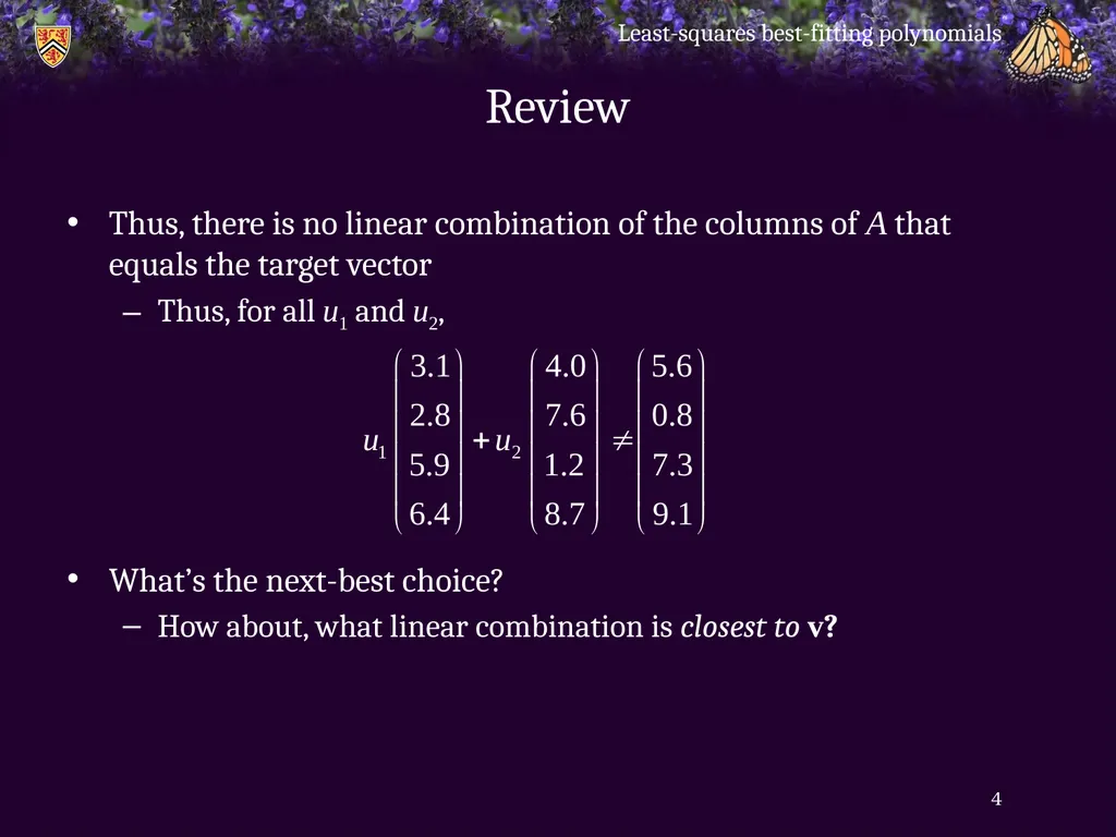
slide4. Review Thus, there is no linear combination of the columns of A that equals the target vector
Thus, for all u1 and u2,
What’s the next-best choice?
How about, what linear combination is closest to v? Least-squares best-fitting polynomials 4<br>
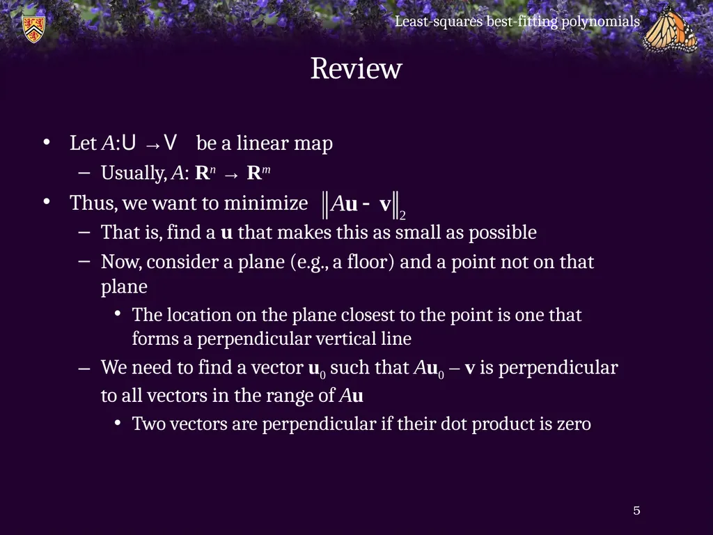
slide5. Review Let A:U →V be a linear map
Usually, A: Rn → Rm
Thus, we want to minimize
That is, find a u that makes this as small as possible
Now, consider a plane (e.g., a floor) and a point not on that plane
The location on the plane closest to the point is one that forms a perpendicular vertical line
We need to find a vector u0 such that Au0 – v is perpendicular to all vectors in the range of Au
Two vectors are perpendicular if their dot product is zero Least-squares best-fitting polynomials 5<br>
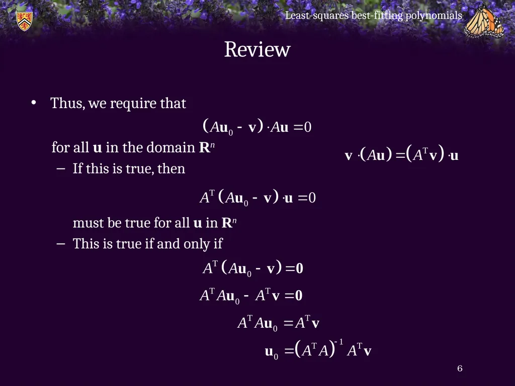
slide6. Review Thus, we require that
for all u in the domain Rn
If this is true, then must be true for all u in Rn
This is true if and only if Least-squares best-fitting polynomials 6<br>
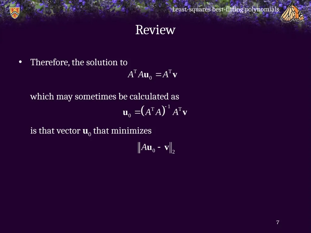
slide7. Review Therefore, the solution to which may sometimes be calculated as is that vector u0 that minimizes Least-squares best-fitting polynomials 7<br>
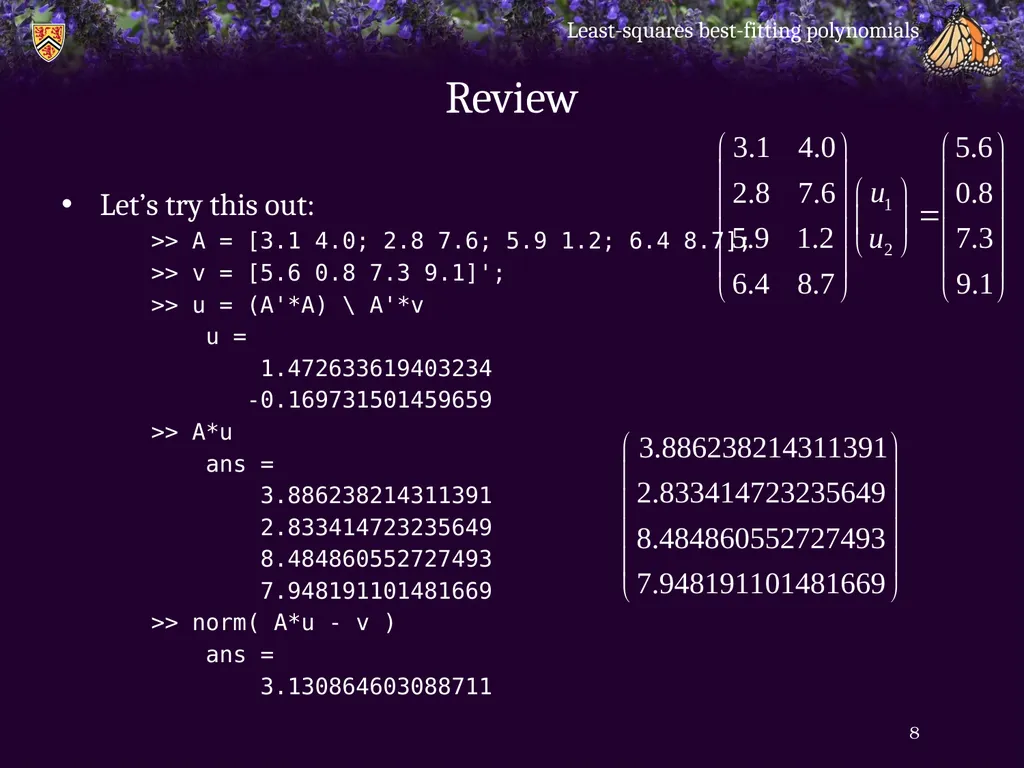
slide8. Review Let’s try this out:
>> A = [3.1 4.0; 2.8 7.6; 5.9 1.2; 6.4 8.7];
>> v = [5.6 0.8 7.3 9.1]';
>> u = (A'*A) \ A'*v
u =
1.472633619403234
-0.169731501459659
>> A*u
ans =
3.886238214311391
2.833414723235649
8.484860552727493
7.948191101481669
>> norm( A*u - v )
ans =
3.130864603088711 Least-squares best-fitting polynomials 8<br>
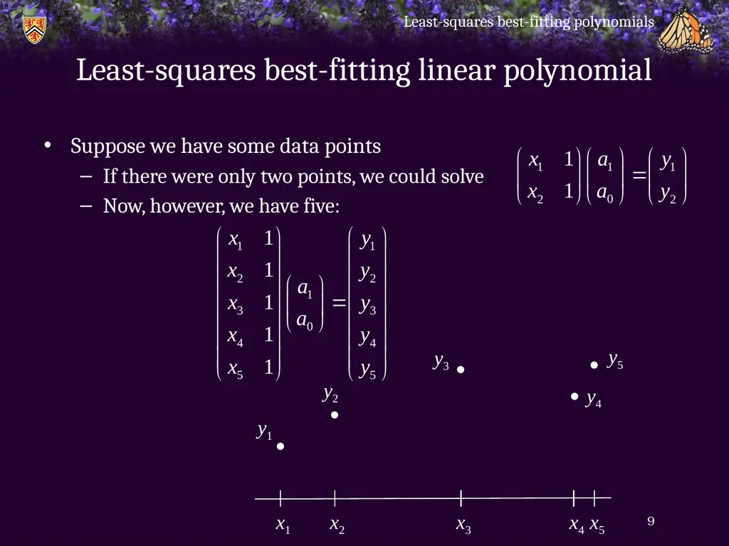
slide9. Least-squares best-fitting linear polynomial Suppose we have some data points
If there were only two points, we could solve
Now, however, we have five: Least-squares best-fitting polynomials 9 x5 x4 x3 x2 x1 y1 y2 y4 y5 y3<br>
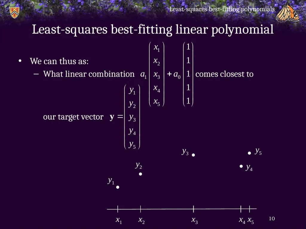
slide10. Least-squares best-fitting linear polynomial We can thus as:
What linear combination comes closest to our target vector Least-squares best-fitting polynomials 10 x5 x4 x3 x2 x1 y1 y2 y4 y5 y3<br>
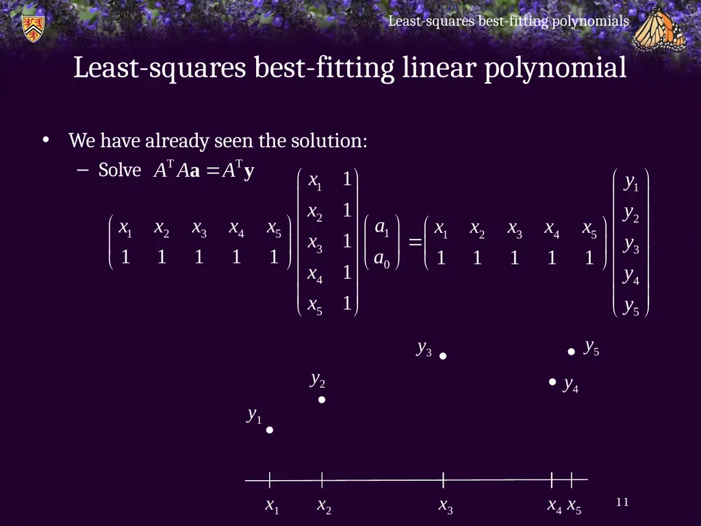
slide11. Least-squares best-fitting linear polynomial We have already seen the solution:
Solve Least-squares best-fitting polynomials 11 x5 x4 x3 x2 x1 y1 y2 y4 y5 y3<br>
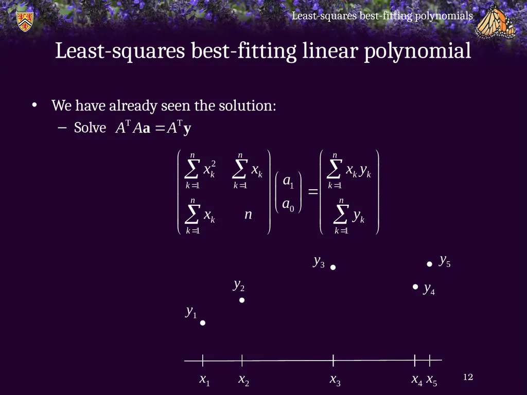
slide12. Least-squares best-fitting linear polynomial We have already seen the solution:
Solve Least-squares best-fitting polynomials 12 x5 x4 x3 x2 x1 y1 y2 y4 y5 y3<br>
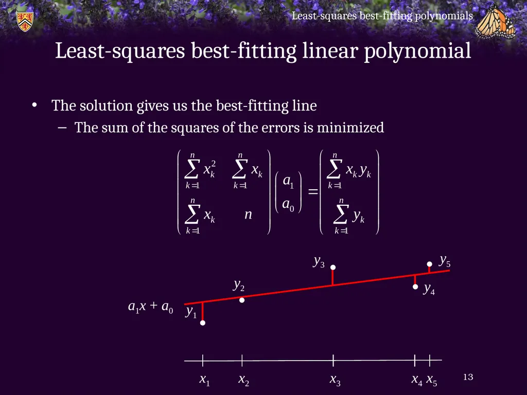
slide13. Least-squares best-fitting linear polynomial The solution gives us the best-fitting line
The sum of the squares of the errors is minimized Least-squares best-fitting polynomials 13 x5 x4 x3 x2 x1 y1 y2 y3 y4 y5 a1x + a0<br>
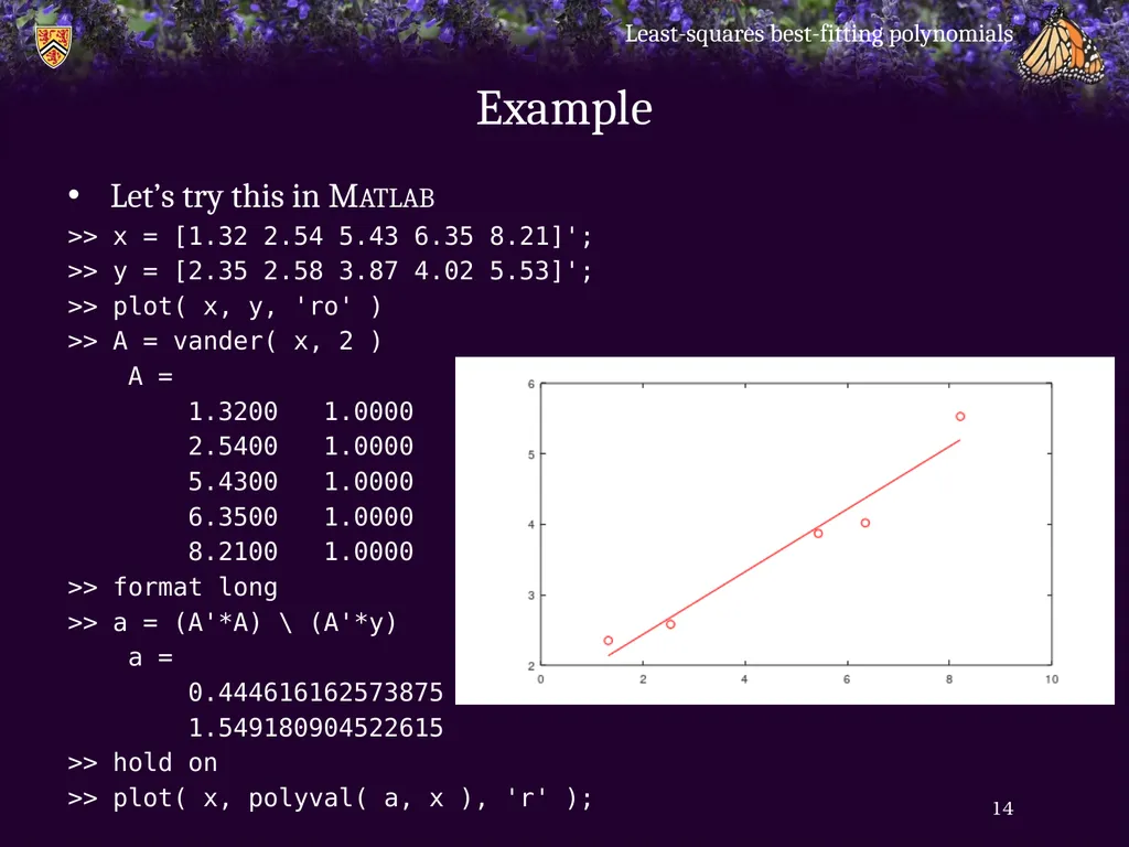
slide14. Example Let’s try this in Matlab
>> x = [1.32 2.54 5.43 6.35 8.21]';
>> y = [2.35 2.58 3.87 4.02 5.53]';
>> plot( x, y, 'ro' )
>> A = vander( x, 2 )
A =
1.3200 1.0000
2.5400 1.0000
5.4300 1.0000
6.3500 1.0000
8.2100 1.0000
>> format long
>> a = (A'*A) \ (A'*y)
a =
0.444616162573875
1.549180904522615
>> hold on
>> plot( x, polyval( a, x ), 'r' ); Least-squares best-fitting polynomials 14<br>
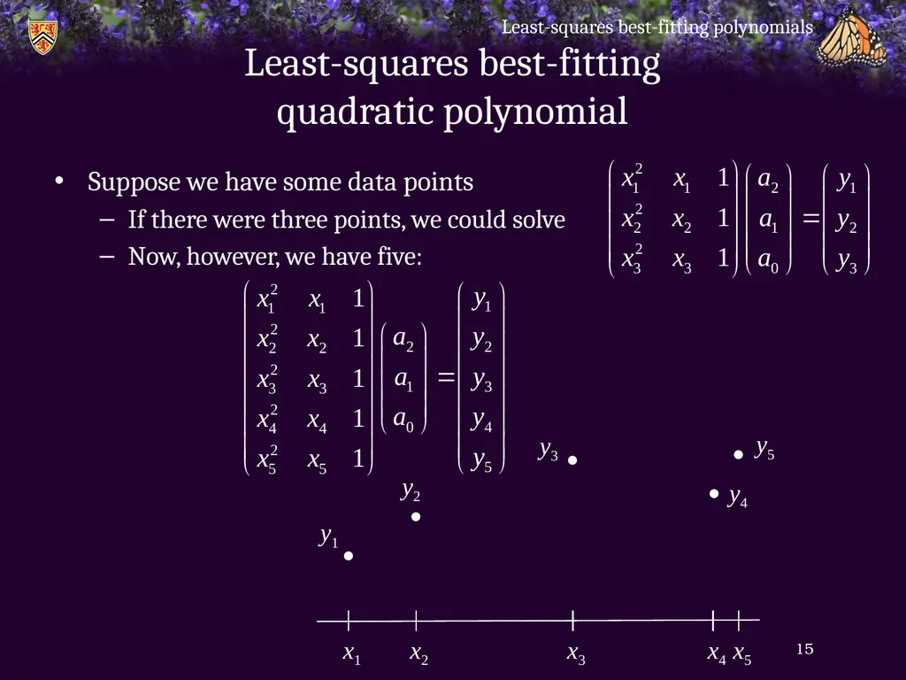
slide15. Least-squares best-fitting quadratic polynomial Suppose we have some data points
If there were three points, we could solve
Now, however, we have five: Least-squares best-fitting polynomials 15 x5 x4 x3 x2 x1 y1 y2 y4 y5 y3<br>
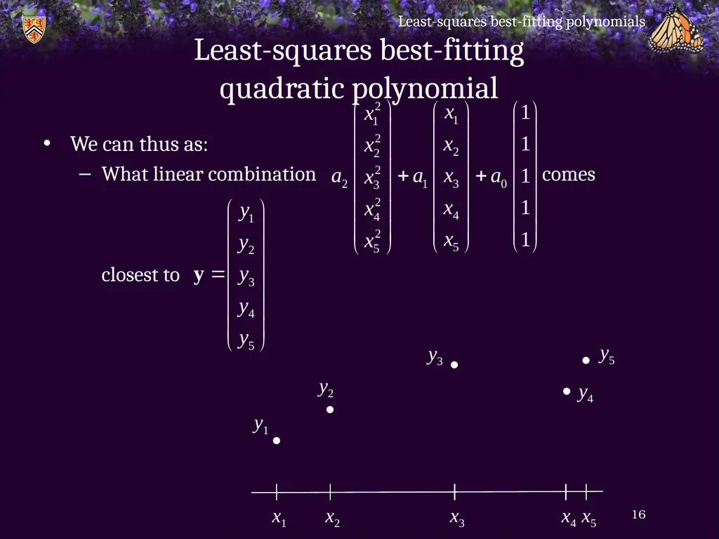
slide16. Least-squares best-fitting quadratic polynomial We can thus as:
What linear combination comes closest to Least-squares best-fitting polynomials 16 x5 x4 x3 x2 x1 y1 y2 y4 y5 y3<br>
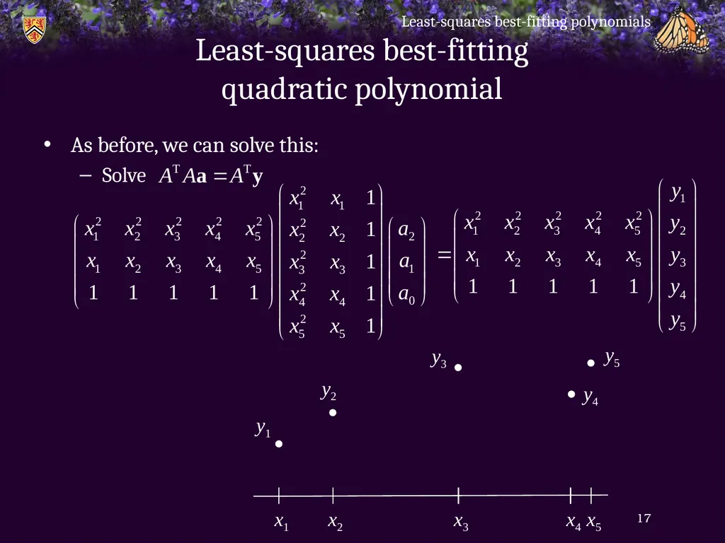
slide17. Least-squares best-fitting quadratic polynomial As before, we can solve this:
Solve Least-squares best-fitting polynomials 17 x5 x4 x3 x2 x1 y1 y2 y4 y5 y3<br>
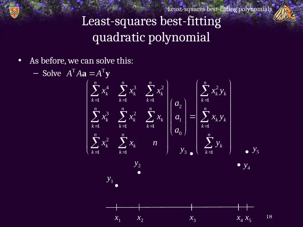
slide18. Least-squares best-fitting quadratic polynomial As before, we can solve this:
Solve Least-squares best-fitting polynomials 18 x5 x4 x3 x2 x1 y1 y2 y4 y5 y3<br>
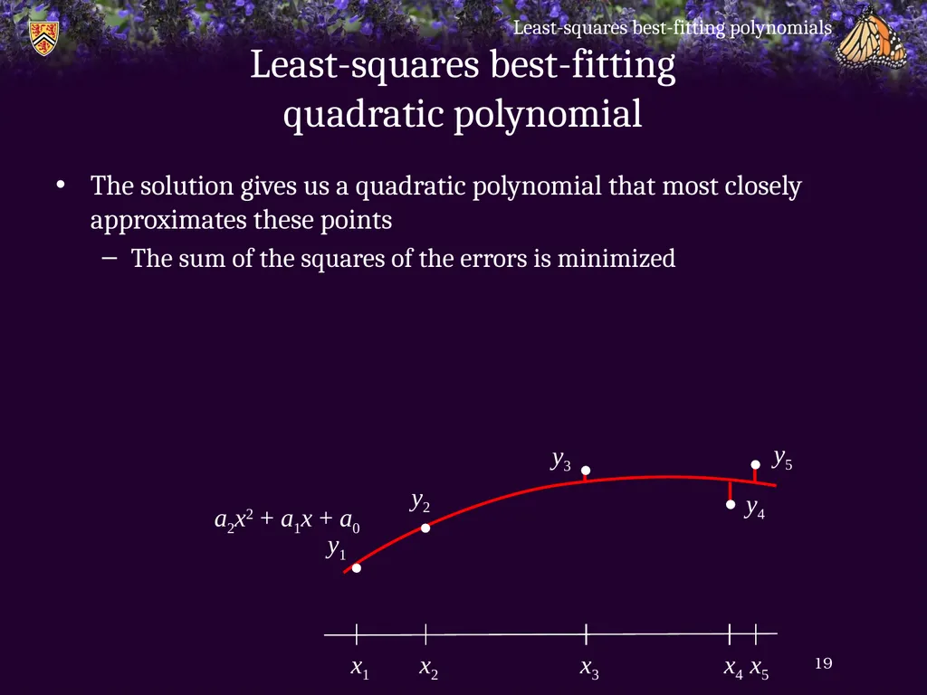
slide19. Least-squares best-fitting quadratic polynomial The solution gives us a quadratic polynomial that most closely approximates these points
The sum of the squares of the errors is minimized Least-squares best-fitting polynomials 19 x5 x4 x3 x2 x1 y1 y2 y3 y4 y5 a2x2 + a1x + a0<br>
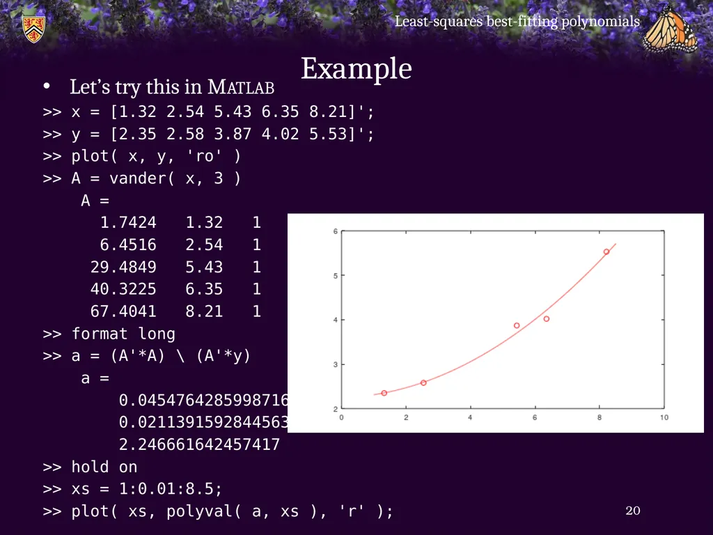
slide20. Example Let’s try this in Matlab
>> x = [1.32 2.54 5.43 6.35 8.21]';
>> y = [2.35 2.58 3.87 4.02 5.53]';
>> plot( x, y, 'ro' )
>> A = vander( x, 3 )
A =
1.7424 1.32 1
6.4516 2.54 1
29.4849 5.43 1
40.3225 6.35 1
67.4041 8.21 1
>> format long
>> a = (A'*A) \ (A'*y)
a =
0.04547642859987164
0.02113915928445630
2.246661642457417
>> hold on
>> xs = 1:0.01:8.5;
>> plot( xs, polyval( a, xs ), 'r' ); Least-squares best-fitting polynomials 20<br>
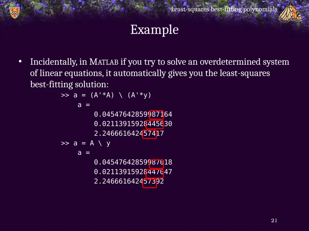
slide21. Example Incidentally, in Matlab if you try to solve an overdetermined system of linear equations, it automatically gives you the least-squares best-fitting solution:
>> a = (A'*A) \ (A'*y)
a =
0.04547642859987164
0.02113915928445630
2.246661642457417
>> a = A \ y
a =
0.04547642859987018
0.02113915928447047
2.246661642457392 Least-squares best-fitting polynomials 21<br>
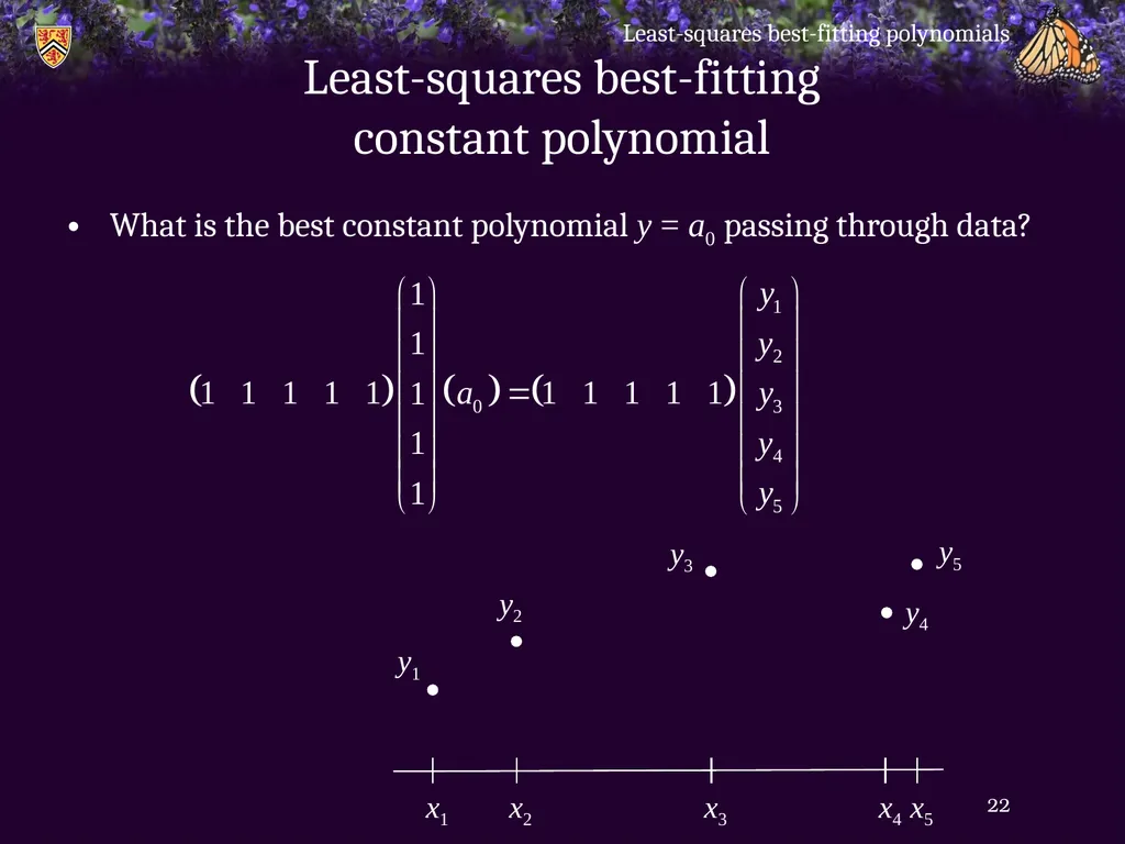
slide22. Least-squares best-fitting constant polynomial What is the best constant polynomial y = a0 passing through data? Least-squares best-fitting polynomials 22 x5 x4 x3 x2 x1 y1 y2 y4 y5 y3<br>
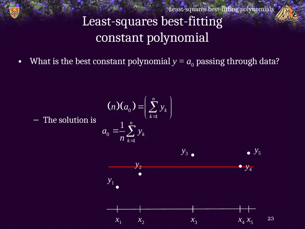
slide23. Least-squares best-fitting constant polynomial What is the best constant polynomial y = a0 passing through data?
The solution is Least-squares best-fitting polynomials 23 x5 x4 x3 x2 x1 y1 y2 y4 y5 y3<br>
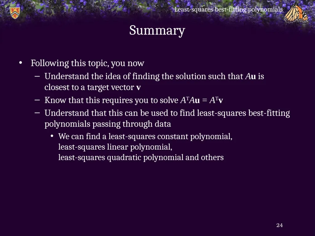
slide24. Summary Following this topic, you now
Understand the idea of finding the solution such that Au is closest to a target vector v
Know that this requires you to solve ATAu = ATv
Understand that this can be used to find least-squares best-fitting polynomials passing through data
We can find a least-squares constant polynomial, least-squares linear polynomial, least-squares quadratic polynomial and others Least-squares best-fitting polynomials 24<br>
slide25. References [1] https://en.wikipedia.org/wiki/Least_squares Least-squares best-fitting polynomials 25<br>
slide26. Acknowledgments None so far. Least-squares best-fitting polynomials 26<br>
slide27. Colophon These slides were prepared using the Cambria typeface. Mathematical equations use Times New Roman, and source code is presented using Consolas. Mathematical equations are prepared in MathType by Design Science, Inc.
Examples may be formulated and checked using Maple by Maplesoft, Inc.
The photographs of flowers and a monarch butter appearing on the title slide and accenting the top of each other slide were taken at the Royal Botanical Gardens in October of 2017 by Douglas Wilhelm Harder. Please see
https://www.rbg.ca/
for more information. Least-squares best-fitting polynomials 27<br>
slide28. Disclaimer These slides are provided for the ece 204 Numerical methods course taught at the University of Waterloo. The material in it reflects the author’s best judgment in light of the information available to them at the time of preparation. Any reliance on these course slides by any party for any other purpose are the responsibility of such parties. The authors accept no responsibility for damages, if any, suffered by any party as a result of decisions made or actions based on these course slides for any other purpose than that for which it was intended. Least-squares best-fitting polynomials 28<br>
slide2. Introduction In this topic, we will
Describe approximating Au = v when no exact solution exists
Introduce the normal equation
Use the normal equation to find the
Best-fitting linear polynomial that fits noisy data
Best-fitting quadratic polynomial that fits noisy data Least-squares best-fitting polynomials 2<br>
slide3. Review From linear algebra:
Suppose that A:R2 → R4 and Au = v has no solution
If the columns of A are linearly independent, this requires that the system is overdetermined with rank 3
That is, there are more equations than unknowns and the system is inconsistent Least-squares best-fitting polynomials 3<br>
slide4. Review Thus, there is no linear combination of the columns of A that equals the target vector
Thus, for all u1 and u2,
What’s the next-best choice?
How about, what linear combination is closest to v? Least-squares best-fitting polynomials 4<br>
slide5. Review Let A:U →V be a linear map
Usually, A: Rn → Rm
Thus, we want to minimize
That is, find a u that makes this as small as possible
Now, consider a plane (e.g., a floor) and a point not on that plane
The location on the plane closest to the point is one that forms a perpendicular vertical line
We need to find a vector u0 such that Au0 – v is perpendicular to all vectors in the range of Au
Two vectors are perpendicular if their dot product is zero Least-squares best-fitting polynomials 5<br>
slide6. Review Thus, we require that
for all u in the domain Rn
If this is true, then must be true for all u in Rn
This is true if and only if Least-squares best-fitting polynomials 6<br>
slide7. Review Therefore, the solution to which may sometimes be calculated as is that vector u0 that minimizes Least-squares best-fitting polynomials 7<br>
slide8. Review Let’s try this out:
>> A = [3.1 4.0; 2.8 7.6; 5.9 1.2; 6.4 8.7];
>> v = [5.6 0.8 7.3 9.1]';
>> u = (A'*A) \ A'*v
u =
1.472633619403234
-0.169731501459659
>> A*u
ans =
3.886238214311391
2.833414723235649
8.484860552727493
7.948191101481669
>> norm( A*u - v )
ans =
3.130864603088711 Least-squares best-fitting polynomials 8<br>
slide9. Least-squares best-fitting linear polynomial Suppose we have some data points
If there were only two points, we could solve
Now, however, we have five: Least-squares best-fitting polynomials 9 x5 x4 x3 x2 x1 y1 y2 y4 y5 y3<br>
slide10. Least-squares best-fitting linear polynomial We can thus as:
What linear combination comes closest to our target vector Least-squares best-fitting polynomials 10 x5 x4 x3 x2 x1 y1 y2 y4 y5 y3<br>
slide11. Least-squares best-fitting linear polynomial We have already seen the solution:
Solve Least-squares best-fitting polynomials 11 x5 x4 x3 x2 x1 y1 y2 y4 y5 y3<br>
slide12. Least-squares best-fitting linear polynomial We have already seen the solution:
Solve Least-squares best-fitting polynomials 12 x5 x4 x3 x2 x1 y1 y2 y4 y5 y3<br>
slide13. Least-squares best-fitting linear polynomial The solution gives us the best-fitting line
The sum of the squares of the errors is minimized Least-squares best-fitting polynomials 13 x5 x4 x3 x2 x1 y1 y2 y3 y4 y5 a1x + a0<br>
slide14. Example Let’s try this in Matlab
>> x = [1.32 2.54 5.43 6.35 8.21]';
>> y = [2.35 2.58 3.87 4.02 5.53]';
>> plot( x, y, 'ro' )
>> A = vander( x, 2 )
A =
1.3200 1.0000
2.5400 1.0000
5.4300 1.0000
6.3500 1.0000
8.2100 1.0000
>> format long
>> a = (A'*A) \ (A'*y)
a =
0.444616162573875
1.549180904522615
>> hold on
>> plot( x, polyval( a, x ), 'r' ); Least-squares best-fitting polynomials 14<br>
slide15. Least-squares best-fitting quadratic polynomial Suppose we have some data points
If there were three points, we could solve
Now, however, we have five: Least-squares best-fitting polynomials 15 x5 x4 x3 x2 x1 y1 y2 y4 y5 y3<br>
slide16. Least-squares best-fitting quadratic polynomial We can thus as:
What linear combination comes closest to Least-squares best-fitting polynomials 16 x5 x4 x3 x2 x1 y1 y2 y4 y5 y3<br>
slide17. Least-squares best-fitting quadratic polynomial As before, we can solve this:
Solve Least-squares best-fitting polynomials 17 x5 x4 x3 x2 x1 y1 y2 y4 y5 y3<br>
slide18. Least-squares best-fitting quadratic polynomial As before, we can solve this:
Solve Least-squares best-fitting polynomials 18 x5 x4 x3 x2 x1 y1 y2 y4 y5 y3<br>
slide19. Least-squares best-fitting quadratic polynomial The solution gives us a quadratic polynomial that most closely approximates these points
The sum of the squares of the errors is minimized Least-squares best-fitting polynomials 19 x5 x4 x3 x2 x1 y1 y2 y3 y4 y5 a2x2 + a1x + a0<br>
slide20. Example Let’s try this in Matlab
>> x = [1.32 2.54 5.43 6.35 8.21]';
>> y = [2.35 2.58 3.87 4.02 5.53]';
>> plot( x, y, 'ro' )
>> A = vander( x, 3 )
A =
1.7424 1.32 1
6.4516 2.54 1
29.4849 5.43 1
40.3225 6.35 1
67.4041 8.21 1
>> format long
>> a = (A'*A) \ (A'*y)
a =
0.04547642859987164
0.02113915928445630
2.246661642457417
>> hold on
>> xs = 1:0.01:8.5;
>> plot( xs, polyval( a, xs ), 'r' ); Least-squares best-fitting polynomials 20<br>
slide21. Example Incidentally, in Matlab if you try to solve an overdetermined system of linear equations, it automatically gives you the least-squares best-fitting solution:
>> a = (A'*A) \ (A'*y)
a =
0.04547642859987164
0.02113915928445630
2.246661642457417
>> a = A \ y
a =
0.04547642859987018
0.02113915928447047
2.246661642457392 Least-squares best-fitting polynomials 21<br>
slide22. Least-squares best-fitting constant polynomial What is the best constant polynomial y = a0 passing through data? Least-squares best-fitting polynomials 22 x5 x4 x3 x2 x1 y1 y2 y4 y5 y3<br>
slide23. Least-squares best-fitting constant polynomial What is the best constant polynomial y = a0 passing through data?
The solution is Least-squares best-fitting polynomials 23 x5 x4 x3 x2 x1 y1 y2 y4 y5 y3<br>
slide24. Summary Following this topic, you now
Understand the idea of finding the solution such that Au is closest to a target vector v
Know that this requires you to solve ATAu = ATv
Understand that this can be used to find least-squares best-fitting polynomials passing through data
We can find a least-squares constant polynomial, least-squares linear polynomial, least-squares quadratic polynomial and others Least-squares best-fitting polynomials 24<br>
slide25. References [1] https://en.wikipedia.org/wiki/Least_squares Least-squares best-fitting polynomials 25<br>
slide26. Acknowledgments None so far. Least-squares best-fitting polynomials 26<br>
slide27. Colophon These slides were prepared using the Cambria typeface. Mathematical equations use Times New Roman, and source code is presented using Consolas. Mathematical equations are prepared in MathType by Design Science, Inc.
Examples may be formulated and checked using Maple by Maplesoft, Inc.
The photographs of flowers and a monarch butter appearing on the title slide and accenting the top of each other slide were taken at the Royal Botanical Gardens in October of 2017 by Douglas Wilhelm Harder. Please see
https://www.rbg.ca/
for more information. Least-squares best-fitting polynomials 27<br>
slide28. Disclaimer These slides are provided for the ece 204 Numerical methods course taught at the University of Waterloo. The material in it reflects the author’s best judgment in light of the information available to them at the time of preparation. Any reliance on these course slides by any party for any other purpose are the responsibility of such parties. The authors accept no responsibility for damages, if any, suffered by any party as a result of decisions made or actions based on these course slides for any other purpose than that for which it was intended. Least-squares best-fitting polynomials 28<br>