
Lecture 15 Sparse Recovery Using Sparse Matrices





Description: Lecture 15 Sparse Recovery Using Sparse Matrices Compressed Sensing: Recap Want to acquire a signal xx1xn Acquisition proceeds by computing Ax of dimension mn From Ax we want to recover an approximation x of x Method: solve the
Related Topics
Download Presentation
"Lecture 15 Sparse Recovery Using Sparse Matrices" is the property of its rightful owner. Permission is granted to download and print the materials on this website for personal, non-commercial use only, and to display it on your personal computer provided you do not modify the materials and that you retain all copyright notices contained in the materials. By downloading content from our website, you accept the terms of this agreement.
Presentation Transcript
slide1. Lecture 15
Sparse Recovery Using Sparse Matrices<br>
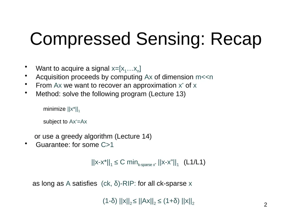
slide2. Compressed Sensing: Recap Want to acquire a signal x=[x1…xn]
Acquisition proceeds by computing Ax of dimension m<<n
From Ax we want to recover an approximation x* of x
Method: solve the following program (Lecture 13)
minimize ||x*||1
subject to Ax*=Ax
or use a greedy algorithm (Lecture 14)
Guarantee: for some C>1
||x-x*||1 ≤ C mink-sparse x” ||x-x”||1 (L1/L1)
as long as A satisfies (ck, δ)-RIP: for all ck-sparse x
(1-δ) ||x||2 ≤ ||Ax||2 ≤ (1+δ) ||x||2 2<br>
slide3. Choices for matrix A Dense matrices:
Compressed sensing
Complexity/learning theory
(Fourier matrices)
Sparse matrices:
Data stream algorithms
Coding theory (LDPCs)
“Traditional” tradeoffs:
Sparse: computationally more efficient ( nlog n vs poly(n) )
Dense: shorter sketches ( k log (n/k) vs k log n)
…
The “best of both worlds” ?<br>
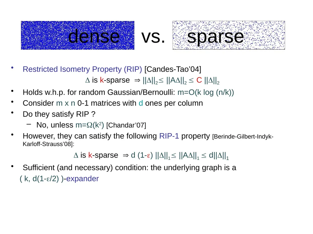
slide4. Restricted Isometry Property (RIP) [Candes-Tao’04]
is k-sparse ||||2 ||A||2 C ||||2
Holds w.h.p. for random Gaussian/Bernoulli: m=O(k log (n/k))
Consider m x n 0-1 matrices with d ones per column
Do they satisfy RIP ?
No, unless m=(k2) [Chandar’07]
However, they can satisfy the following RIP-1 property [Berinde-Gilbert-Indyk-Karloff-Strauss’08]:
is k-sparse d (1-) ||||1 ||A||1 d||||1
Sufficient (and necessary) condition: the underlying graph is a
( k, d(1-/2) )-expander dense vs. sparse<br>
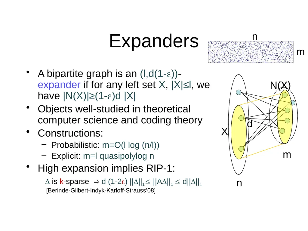
slide5. Expanders A bipartite graph is an (l,d(1-))-expander if for any left set X, |X|≤l, we have |N(X)|≥(1-)d |X|
Objects well-studied in theoretical computer science and coding theory
Constructions:
Probabilistic: m=O(l log (n/l))
Explicit: m=l quasipolylog n
High expansion implies RIP-1:
is k-sparse d (1-2) ||||1 ||A||1 d||||1
[Berinde-Gilbert-Indyk-Karloff-Strauss’08] n m d n m<br>
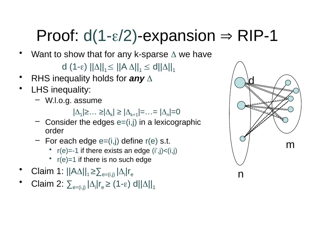
slide6. Proof: d(1-/2)-expansion RIP-1 Want to show that for any k-sparse we have
d (1-) ||||1 ||A ||1 d||||1
RHS inequality holds for any
LHS inequality:
W.l.o.g. assume
|1|≥… ≥|k| ≥ |k+1|=…= |n|=0
Consider the edges e=(i,j) in a lexicographic order
For each edge e=(i,j) define r(e) s.t.
r(e)=-1 if there exists an edge (i’,j)<(i,j)
r(e)=1 if there is no such edge
Claim 1: ||A||1 ≥∑e=(i,j) |i|re
Claim 2: ∑e=(i,j) |i|re ≥ (1-) d||||1 n m d<br>
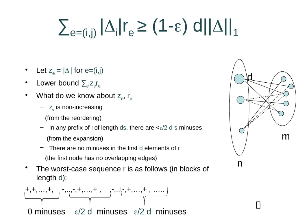
slide7. ∑e=(i,j) |i|re ≥ (1-) d||||1 Let ze = |i| for e=(i,j)
Lower bound ∑e zere
What do we know about ze, re
ze is non-increasing
(from the reordering)
In any prefix of r of length ds, there are </2 d s minuses
(from the expansion)
There are no minuses in the first d elements of r
(the first node has no overlapping edges)
The worst-case sequence r is as follows (in blocks of length d):
+,+,…,+, -,..,-,+,…,+ , ,-,..,-,+,…,+ , ….. n m d 0 minuses /2 d minuses /2 d minuses <br>
slide8. Implication of RIP-1 We have RIP in the L1 norm
Now what ?
We will show that RIP-1 for expander matrices can be used to show null space property (notes), and therefore L1 minimization works
Altogether, this gives a a scheme with:
O(k log (n/k) ) measurements
Recovery time still poly(n)
However, thanks to the use of sparse matrices, the running time is faster
(the linear program iteratively computers Az for vectors z, which is fast if A is sparse)
Coordinate-wise updates are significantly faster<br>
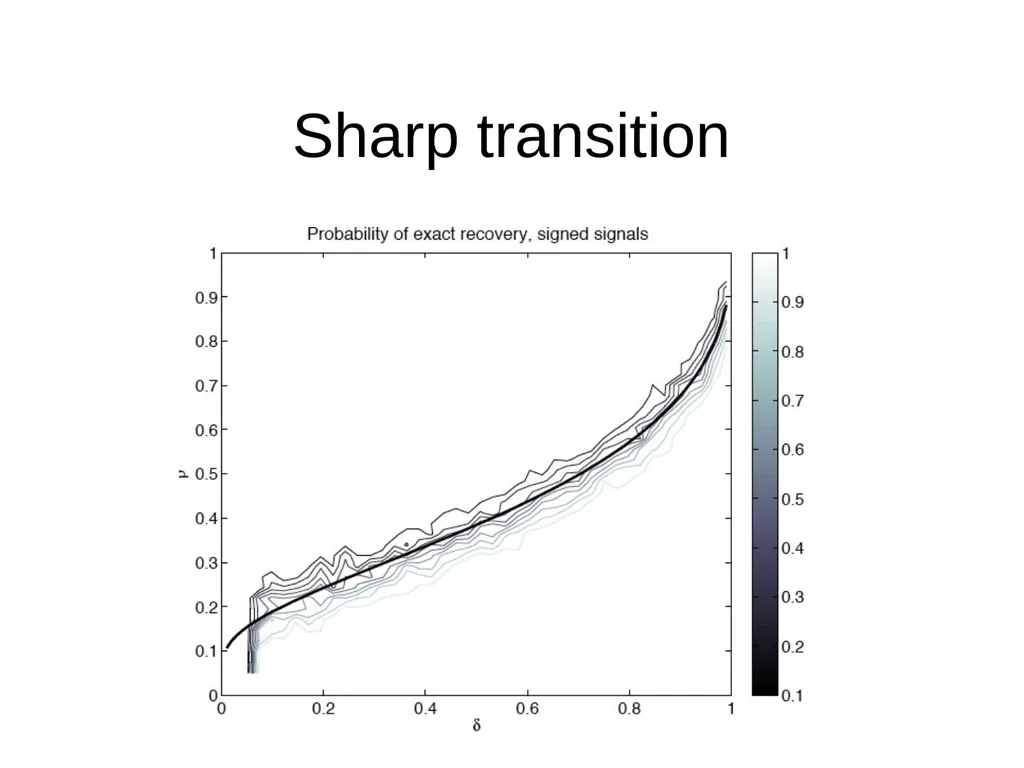
slide9. Sharp transition<br>
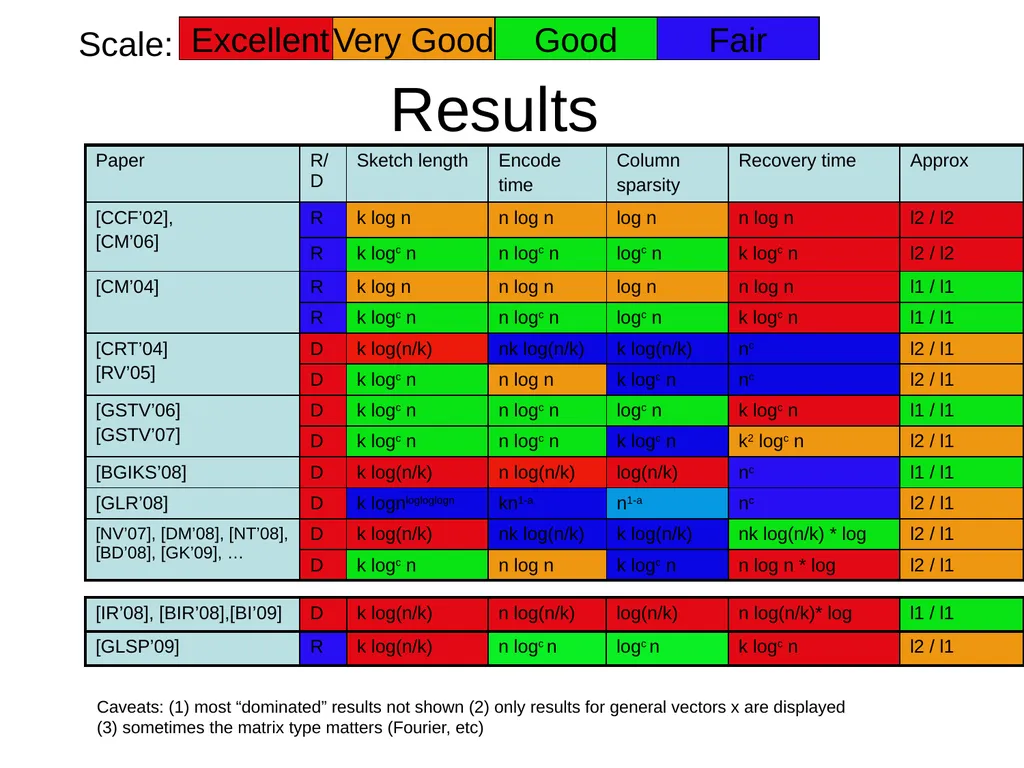
slide10. Results Excellent Scale: Very Good Good Fair Caveats: (1) most “dominated” results not shown (2) only results for general vectors x are displayed
(3) sometimes the matrix type matters (Fourier, etc)<br>
slide11. Application: Monitoring Network Traffic Data Streams Router routs packets
Where do they come from ?
Where do they go to ?
Ideally, would like to maintain a traffic
matrix x[.,.]
Easy to update: given a (src,dst) packet, increment xsrc,dst
Requires way too much space!
(232 x 232 entries)
Need to compress x, increment easily
Using linear compression we can:
Maintain sketch Ax under increments to x, since
A(x+) = Ax + A
Recover x* from Ax source destination x<br>
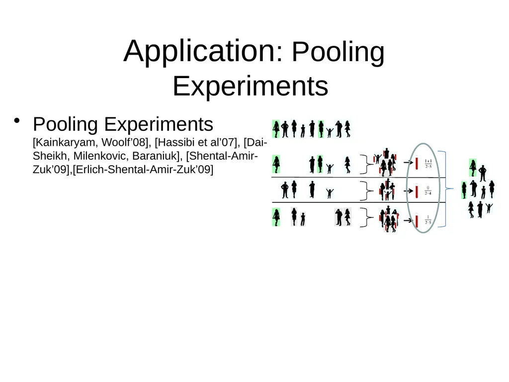
slide12. Application: Pooling Experiments Pooling Experiments [Kainkaryam, Woolf’08], [Hassibi et al’07], [Dai-Sheikh, Milenkovic, Baraniuk], [Shental-Amir-Zuk’09],[Erlich-Shental-Amir-Zuk’09]<br>
slide13. References Survey:
A. Gilbert, P. Indyk, “Sparse recovery using sparse matrices”, Proceedings of IEEE, June 2010.<br>
slide2. Compressed Sensing: Recap Want to acquire a signal x=[x1…xn]
Acquisition proceeds by computing Ax of dimension m<<n
From Ax we want to recover an approximation x* of x
Method: solve the following program (Lecture 13)
minimize ||x*||1
subject to Ax*=Ax
or use a greedy algorithm (Lecture 14)
Guarantee: for some C>1
||x-x*||1 ≤ C mink-sparse x” ||x-x”||1 (L1/L1)
as long as A satisfies (ck, δ)-RIP: for all ck-sparse x
(1-δ) ||x||2 ≤ ||Ax||2 ≤ (1+δ) ||x||2 2<br>
slide3. Choices for matrix A Dense matrices:
Compressed sensing
Complexity/learning theory
(Fourier matrices)
Sparse matrices:
Data stream algorithms
Coding theory (LDPCs)
“Traditional” tradeoffs:
Sparse: computationally more efficient ( nlog n vs poly(n) )
Dense: shorter sketches ( k log (n/k) vs k log n)
…
The “best of both worlds” ?<br>
slide4. Restricted Isometry Property (RIP) [Candes-Tao’04]
is k-sparse ||||2 ||A||2 C ||||2
Holds w.h.p. for random Gaussian/Bernoulli: m=O(k log (n/k))
Consider m x n 0-1 matrices with d ones per column
Do they satisfy RIP ?
No, unless m=(k2) [Chandar’07]
However, they can satisfy the following RIP-1 property [Berinde-Gilbert-Indyk-Karloff-Strauss’08]:
is k-sparse d (1-) ||||1 ||A||1 d||||1
Sufficient (and necessary) condition: the underlying graph is a
( k, d(1-/2) )-expander dense vs. sparse<br>
slide5. Expanders A bipartite graph is an (l,d(1-))-expander if for any left set X, |X|≤l, we have |N(X)|≥(1-)d |X|
Objects well-studied in theoretical computer science and coding theory
Constructions:
Probabilistic: m=O(l log (n/l))
Explicit: m=l quasipolylog n
High expansion implies RIP-1:
is k-sparse d (1-2) ||||1 ||A||1 d||||1
[Berinde-Gilbert-Indyk-Karloff-Strauss’08] n m d n m<br>
slide6. Proof: d(1-/2)-expansion RIP-1 Want to show that for any k-sparse we have
d (1-) ||||1 ||A ||1 d||||1
RHS inequality holds for any
LHS inequality:
W.l.o.g. assume
|1|≥… ≥|k| ≥ |k+1|=…= |n|=0
Consider the edges e=(i,j) in a lexicographic order
For each edge e=(i,j) define r(e) s.t.
r(e)=-1 if there exists an edge (i’,j)<(i,j)
r(e)=1 if there is no such edge
Claim 1: ||A||1 ≥∑e=(i,j) |i|re
Claim 2: ∑e=(i,j) |i|re ≥ (1-) d||||1 n m d<br>
slide7. ∑e=(i,j) |i|re ≥ (1-) d||||1 Let ze = |i| for e=(i,j)
Lower bound ∑e zere
What do we know about ze, re
ze is non-increasing
(from the reordering)
In any prefix of r of length ds, there are </2 d s minuses
(from the expansion)
There are no minuses in the first d elements of r
(the first node has no overlapping edges)
The worst-case sequence r is as follows (in blocks of length d):
+,+,…,+, -,..,-,+,…,+ , ,-,..,-,+,…,+ , ….. n m d 0 minuses /2 d minuses /2 d minuses <br>
slide8. Implication of RIP-1 We have RIP in the L1 norm
Now what ?
We will show that RIP-1 for expander matrices can be used to show null space property (notes), and therefore L1 minimization works
Altogether, this gives a a scheme with:
O(k log (n/k) ) measurements
Recovery time still poly(n)
However, thanks to the use of sparse matrices, the running time is faster
(the linear program iteratively computers Az for vectors z, which is fast if A is sparse)
Coordinate-wise updates are significantly faster<br>
slide9. Sharp transition<br>
slide10. Results Excellent Scale: Very Good Good Fair Caveats: (1) most “dominated” results not shown (2) only results for general vectors x are displayed
(3) sometimes the matrix type matters (Fourier, etc)<br>
slide11. Application: Monitoring Network Traffic Data Streams Router routs packets
Where do they come from ?
Where do they go to ?
Ideally, would like to maintain a traffic
matrix x[.,.]
Easy to update: given a (src,dst) packet, increment xsrc,dst
Requires way too much space!
(232 x 232 entries)
Need to compress x, increment easily
Using linear compression we can:
Maintain sketch Ax under increments to x, since
A(x+) = Ax + A
Recover x* from Ax source destination x<br>
slide12. Application: Pooling Experiments Pooling Experiments [Kainkaryam, Woolf’08], [Hassibi et al’07], [Dai-Sheikh, Milenkovic, Baraniuk], [Shental-Amir-Zuk’09],[Erlich-Shental-Amir-Zuk’09]<br>
slide13. References Survey:
A. Gilbert, P. Indyk, “Sparse recovery using sparse matrices”, Proceedings of IEEE, June 2010.<br>