Linear Programming Jeff Edmonds York University

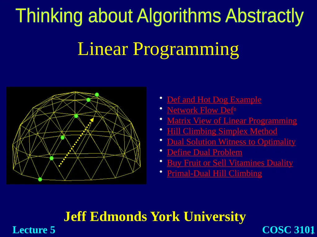
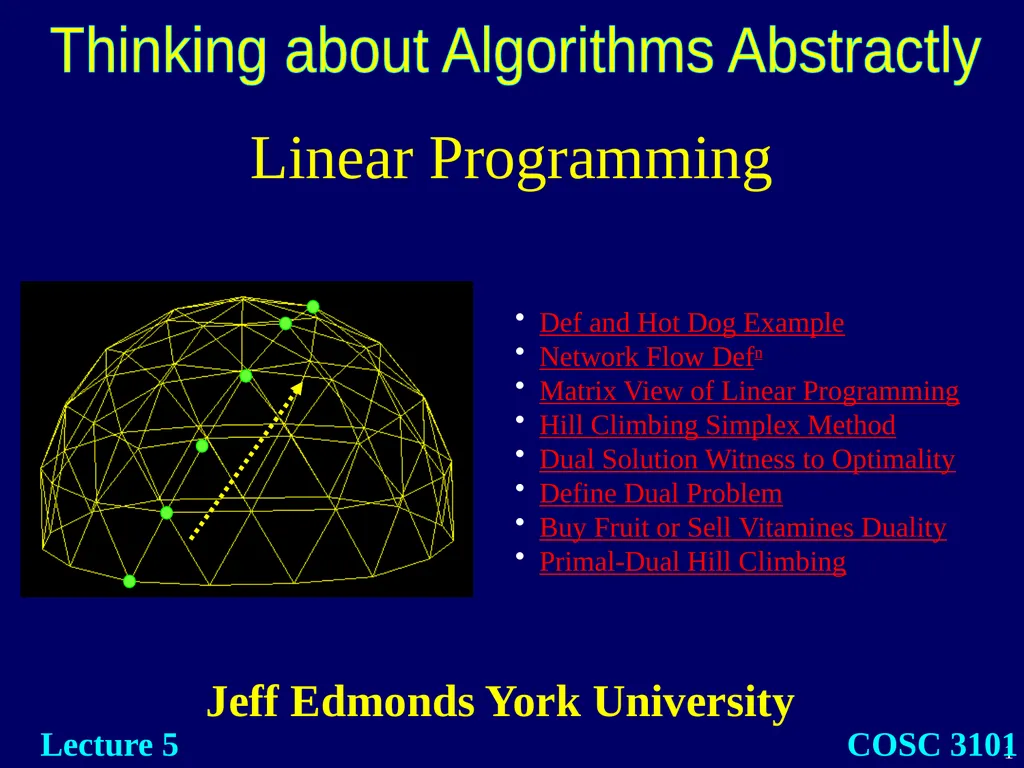
slide1. Linear Programming Jeff Edmonds York University COSC 3101 Lecture 5 Thinking about Algorithms Abstractly Def and Hot Dog Example
Network Flow Defn
Matrix View of Linear Programming
Hill Climbing Simplex Method
Dual Solution Witness to Optimality
Define Dual Problem
Buy Fruit or Sell Vitamines Duality
Primal-Dual Hill Climbing<br>
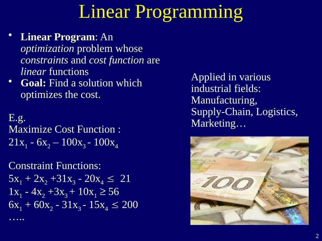
slide2. Linear Programming Linear Program: An optimization problem whose constraints and cost function are linear functions
Goal: Find a solution which optimizes the cost.

E.g.
Maximize Cost Function :
21x1 - 6x2 – 100x3 - 100x4

Constraint Functions:
5x1 + 2x2 +31x3 - 20x4  21
1x1 - 4x2 +3x3 + 10x1 ³ 56
6x1 + 60x2 - 31x3 - 15x4  200
…..<br>
slide3. A Hotdog A combination of pork, grain, and sawdust, …<br>
slide4. Constraints:
Amount of moisture
Amount of protein,
…<br>
slide5. The Hotdog Problem Given today’s prices,what is a fast algorithm to find the cheapest hotdog?<br>
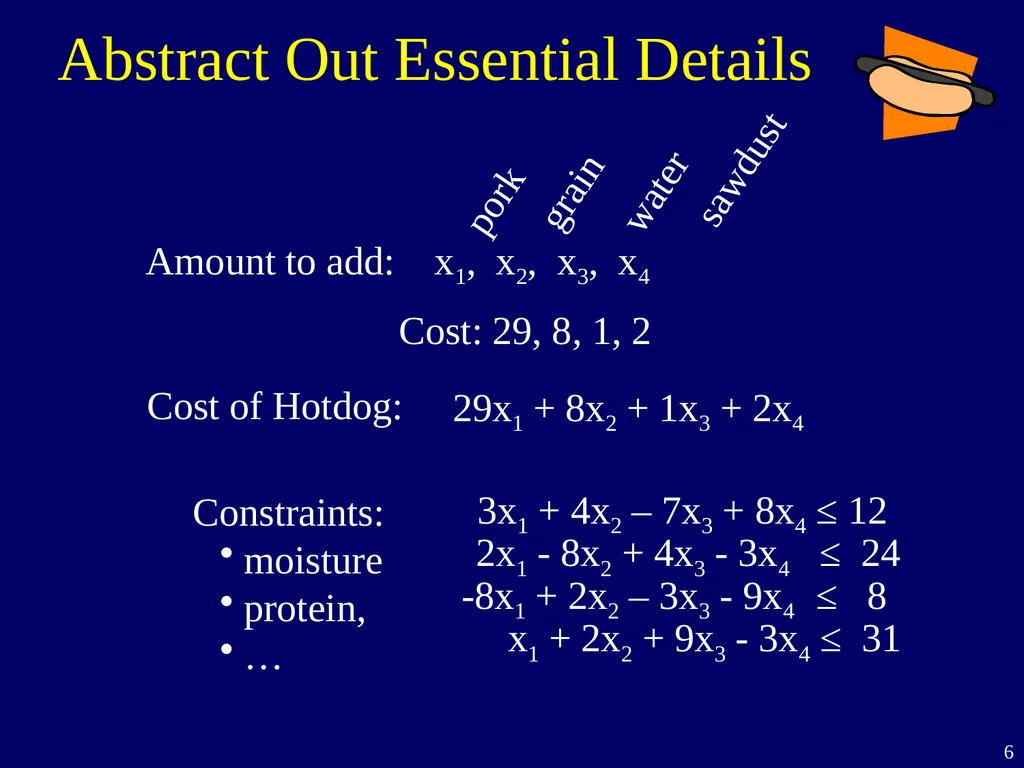
slide6. Abstract Out Essential Details Cost: 29, 8, 1, 2<br>
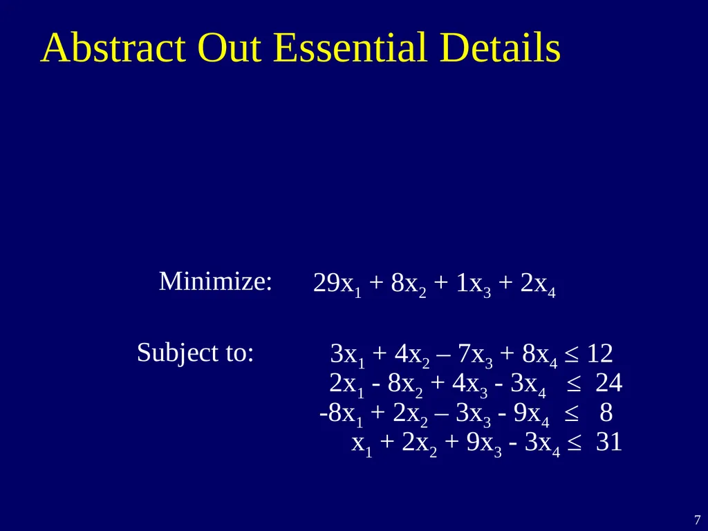
slide7. 29x1 + 8x2 + 1x3 + 2x4 Subject to: Minimize: Abstract Out Essential Details<br>
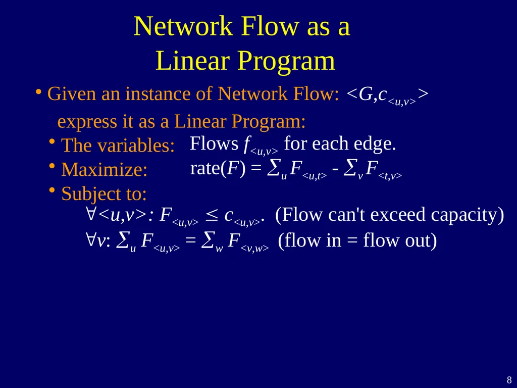
slide8. Network Flow as a Linear Program Given an instance of Network Flow: <G,c<u,v>> express it as a Linear Program:
The variables:
Maximize:
Subject to: Flows f<u,v> for each edge. <u,v>: F<u,v>  c<u,v>. (Flow can't exceed capacity) v: u F<u,v> = w F<v,w> (flow in = flow out) rate(F) = u F<u,t> - v F<t,v><br>
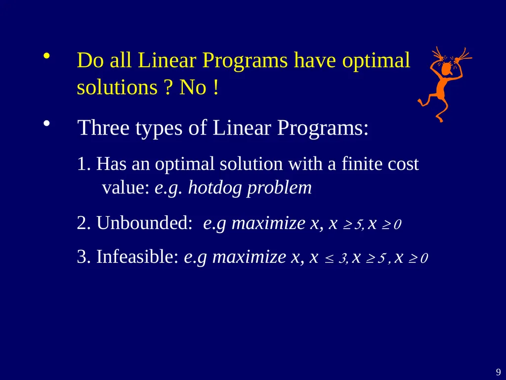
slide9. Do all Linear Programs have optimal solutions ? No ! Three types of Linear Programs: 1. Has an optimal solution with a finite cost value: e.g. hotdog problem 2. Unbounded: e.g maximize x, x ³ 5, x ³ 0 3. Infeasible: e.g maximize x, x  3, x ³ 5 , x ³ 0<br>
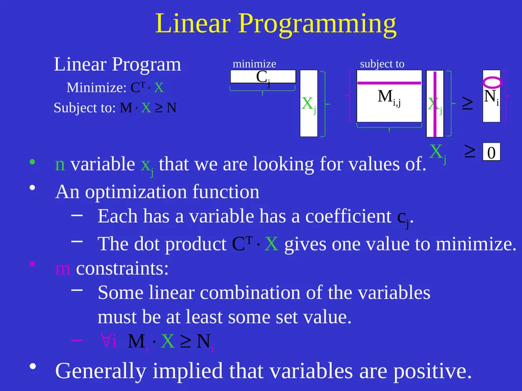
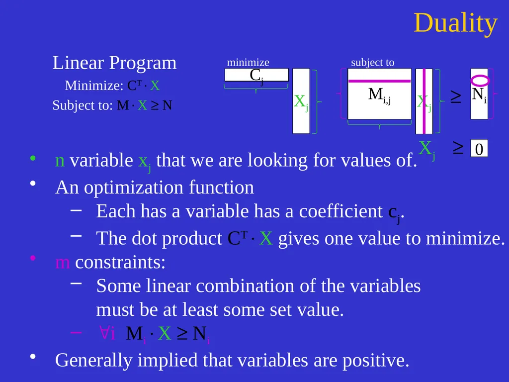
slide10. Linear Programming Linear Program
Minimize: CTX
Subject to: MX ³ N n variable xj that we are looking for values of.
An optimization function
Each has a variable has a coefficient cj.
The dot product CTX gives one value to minimize.
m constraints:
Some linear combination of the variablesmust be at least some set value.
i MiX ³ Ni
Generally implied that variables are positive.<br>
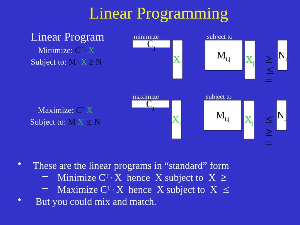
slide11. Linear Programming Linear Program
Minimize: CTX
Subject to: MX ³ N These are the linear programs in “standard” form
Minimize CTX hence X subject to X ³
Maximize CTX hence X subject to X 
But you could mix and match. Xj<br>
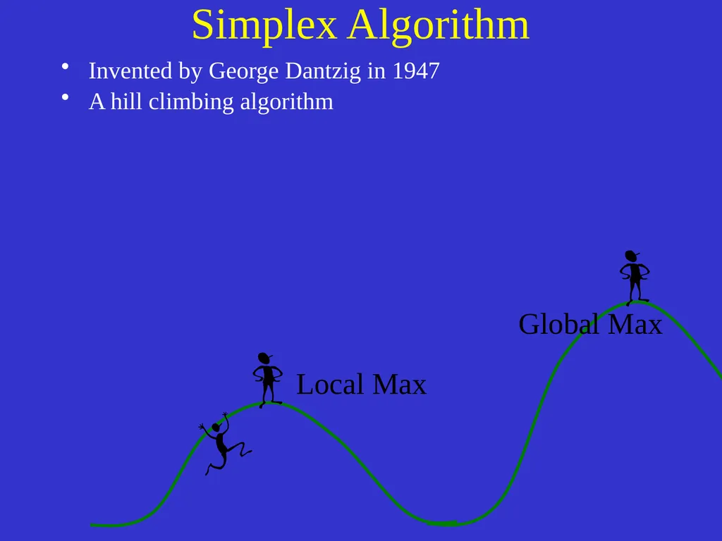
slide12. Simplex Algorithm Invented by George Dantzig in 1947
A hill climbing algorithm Local Max Global Max<br>
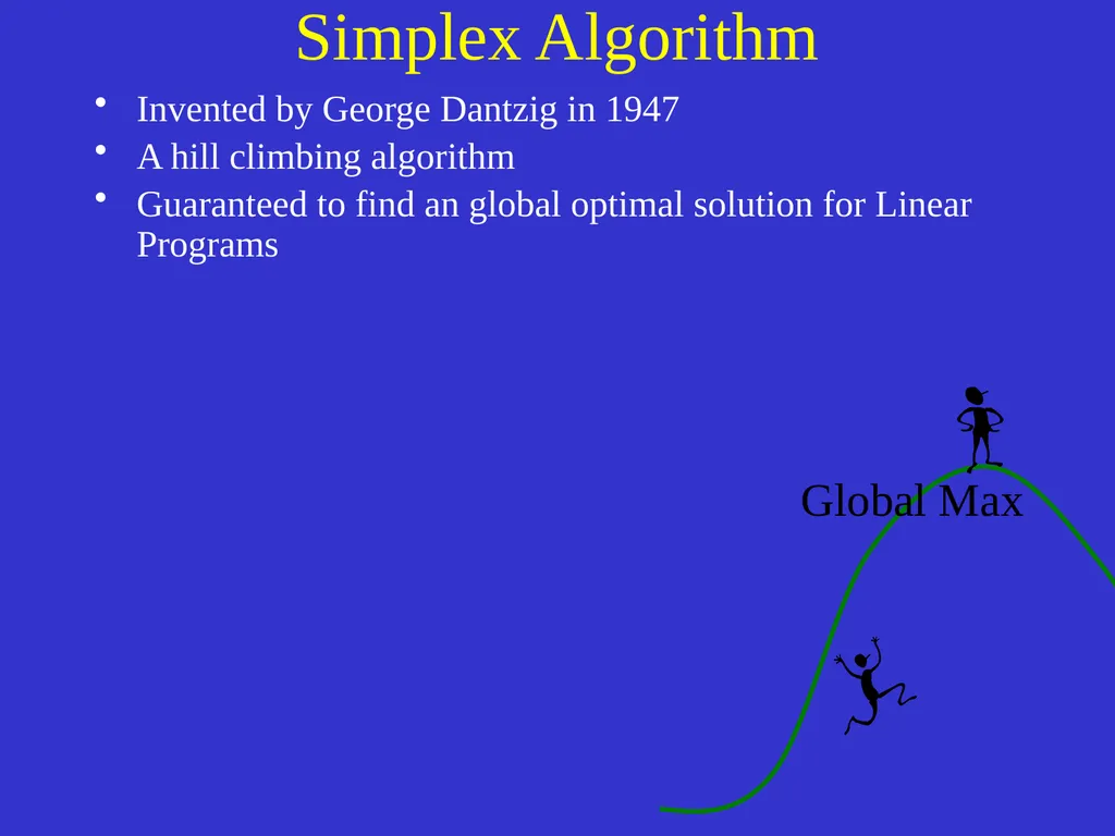
slide13. Simplex Algorithm Invented by George Dantzig in 1947
A hill climbing algorithm
Guaranteed to find an global optimal solution for Linear Programs Global Max<br>
slide14. Simplex Algorithm<br>
slide15. Minimize
Cost = 5x1 + 7x2

Constraint Functions
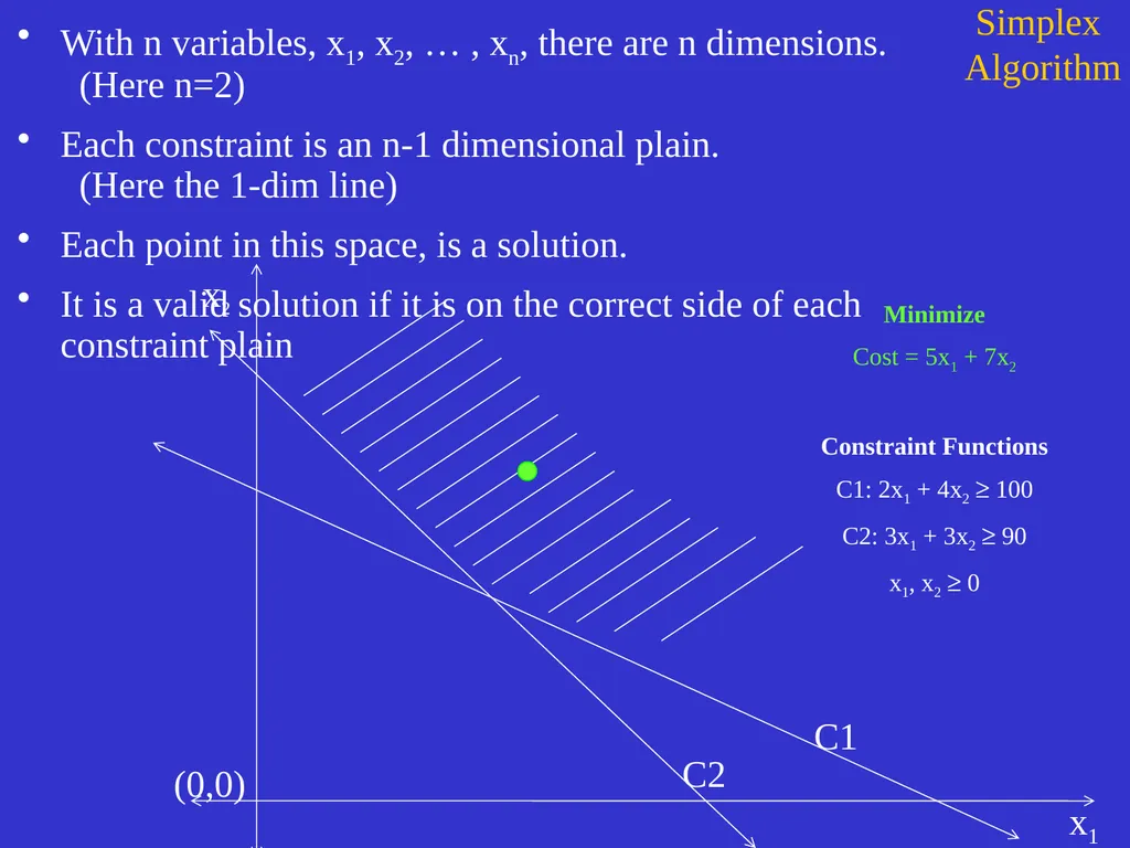
C1: 2x1 + 4x2 ³ 100
C2: 3x1 + 3x2 ³ 90
x1, x2 ³ 0 With n variables, x1, x2, … , xn, there are n dimensions. (Here n=2)
Each constraint is an n-1 dimensional plain. (Here the 1-dim line)
Each point in this space, is a solution.
It is a valid solution if it is on the correct side of each constraint plain Simplex Algorithm<br>
slide16. C1 C2 (0,0) x2 x1 Cost Function
Cost = 5x1 + 7x2

Constraint Functions
C1: 2x1 + 4x2 ³ 100
C2: 3x1 + 3x2 ³ 90
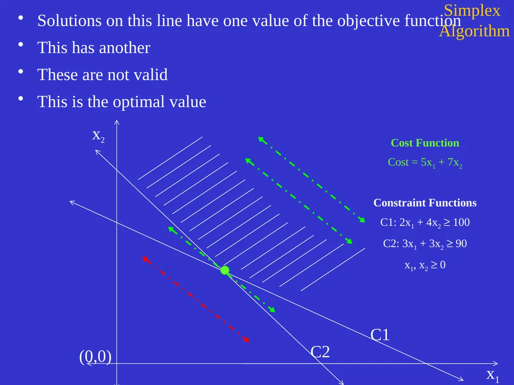
x1, x2 ³ 0 Solutions on this line have one value of the objective function
This has another
These are not valid
This is the optimal value Simplex Algorithm<br>
slide17. C1 C2 (0,0) x2 x1 Cost Function
Cost = 5x1 + 7x2

Constraint Functions
C1: 2x1 + 4x2 ³ 100
C2: 3x1 + 3x2 ³ 90
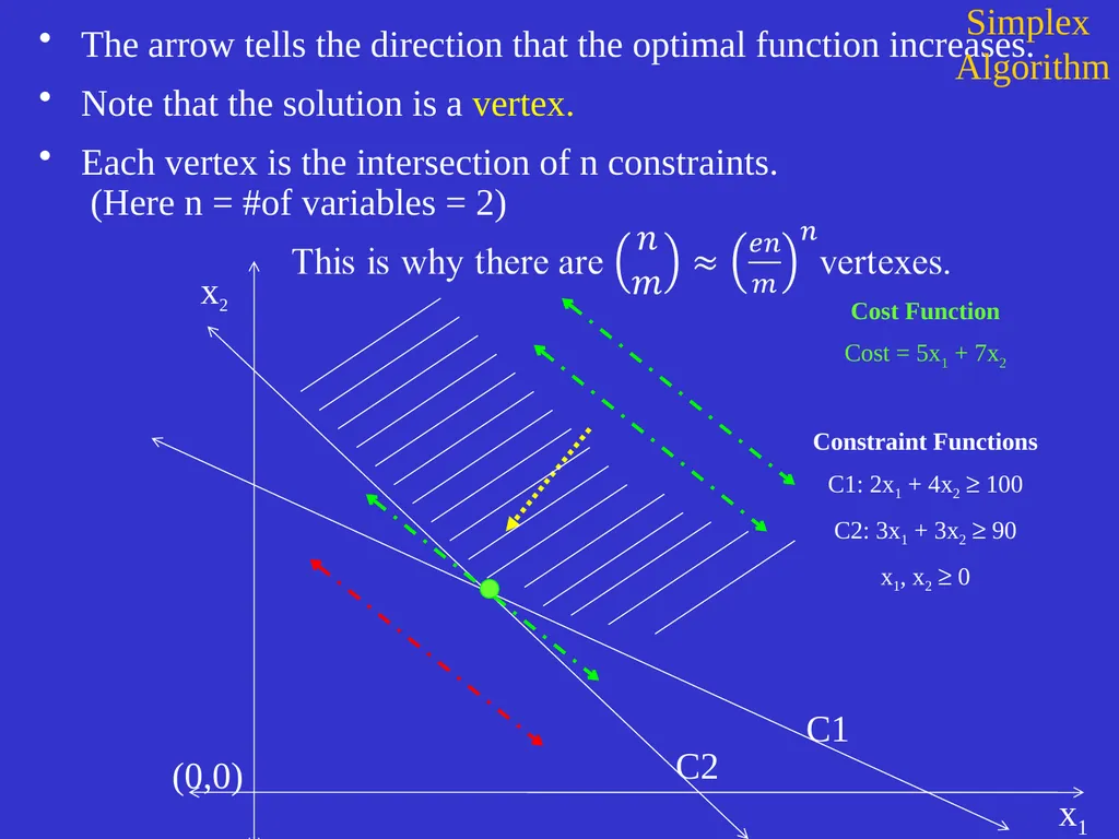
x1, x2 ³ 0 The arrow tells the direction that the optimal function increases.
Note that the solution is a vertex.
Each vertex is the intersection of n constraints. (Here n = #of variables = 2) Simplex Algorithm<br>
slide18. The arrow tells the direction that the optimal function increases.
Note that the solution is a vertex.
Each vertex is the intersection of n constraints. (Here n = #of variables = 2)
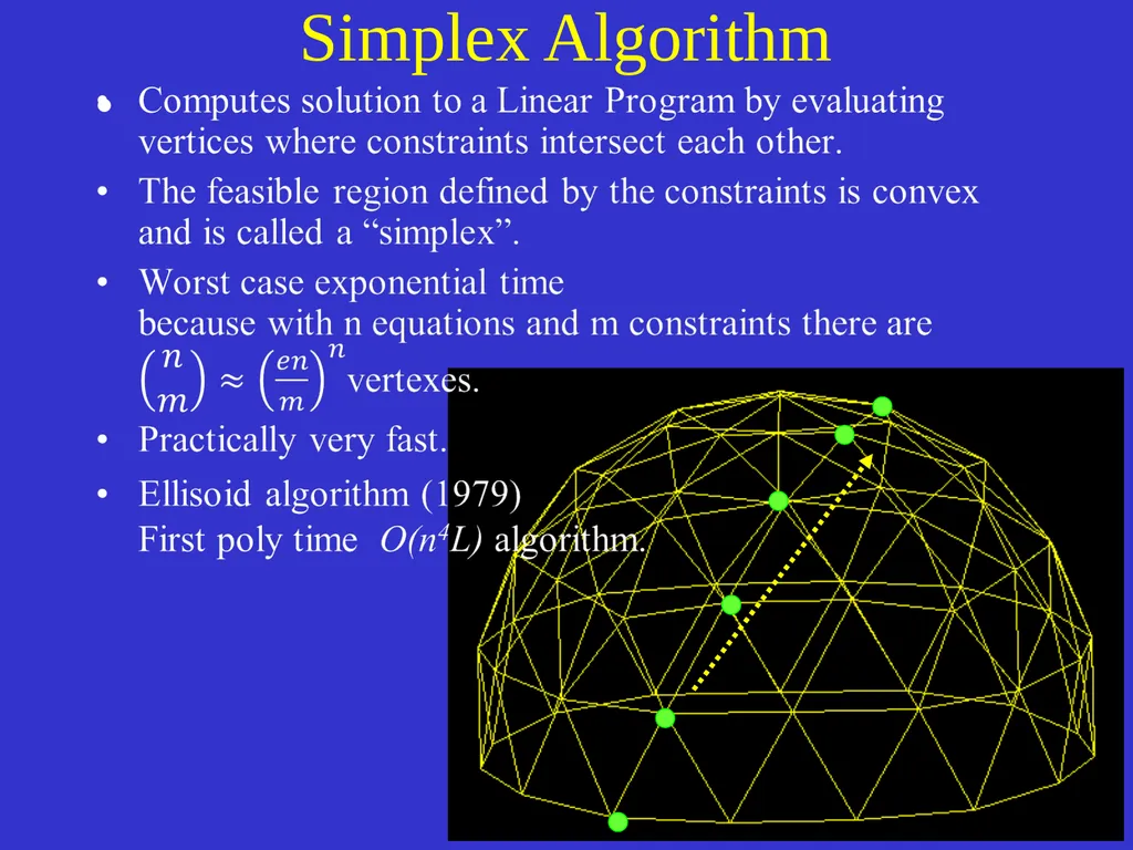
The simplex method takes hill climbing steps, from one vertex (valid solution) to another. vertex Algorithm<br>
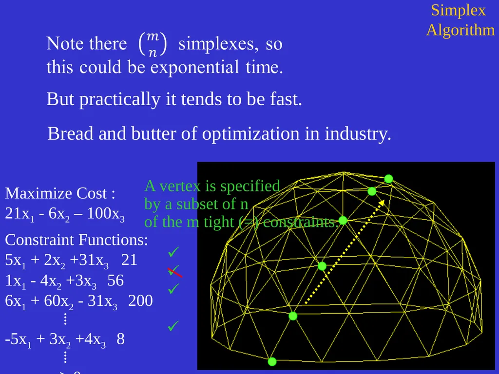
slide19. Maximize Cost : 21x1 - 6x2 – 100x3
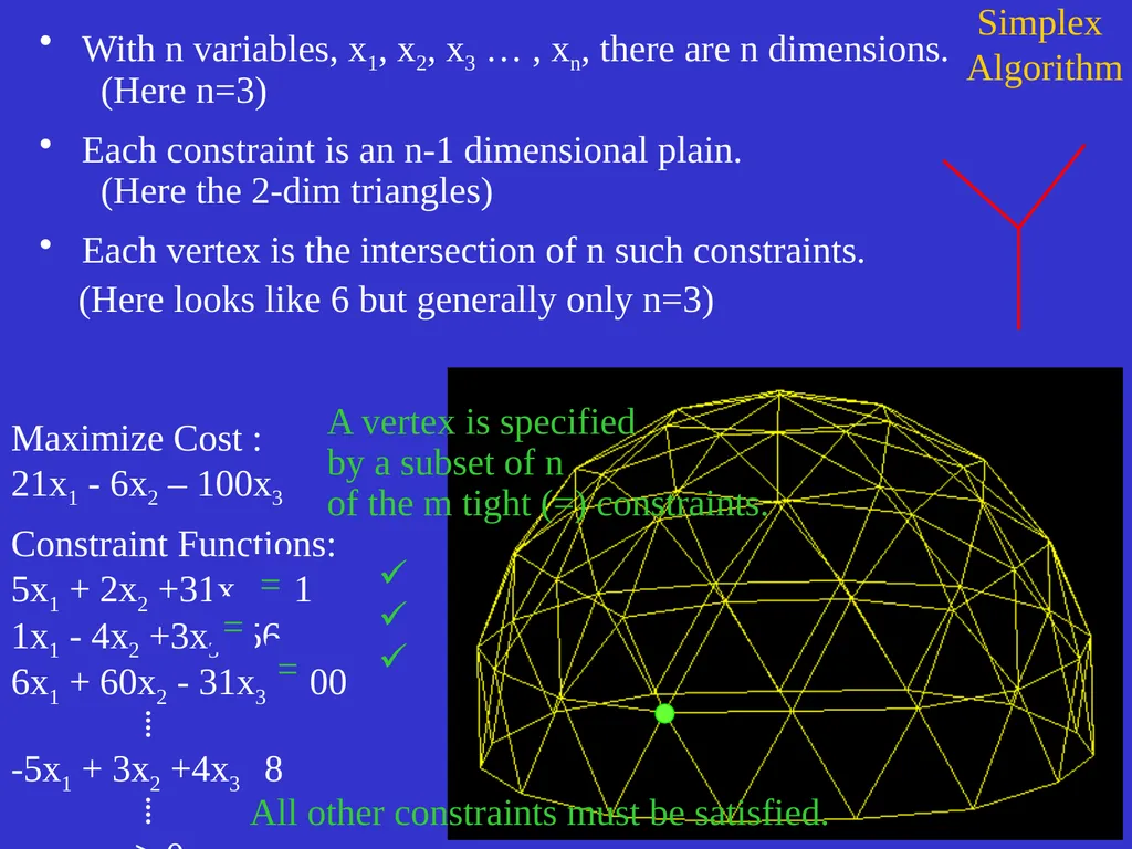
Constraint Functions:5x1 + 2x2 +31x3  211x1 - 4x2 +3x3  566x1 + 60x2 - 31x3  200 ⁞-5x1 + 3x2 +4x3  8 ⁞x1, x2, x3 ³ 0 With n variables, x1, x2, x3 … , xn, there are n dimensions. (Here n=3)
Each constraint is an n-1 dimensional plain. (Here the 2-dim triangles)
Each vertex is the intersection of n such constraints. (Here looks like 6 but generally only n=3) Simplex Algorithm All other constraints must be satisfied.<br>
slide20. Maximize Cost : 21x1 - 6x2 – 100x3
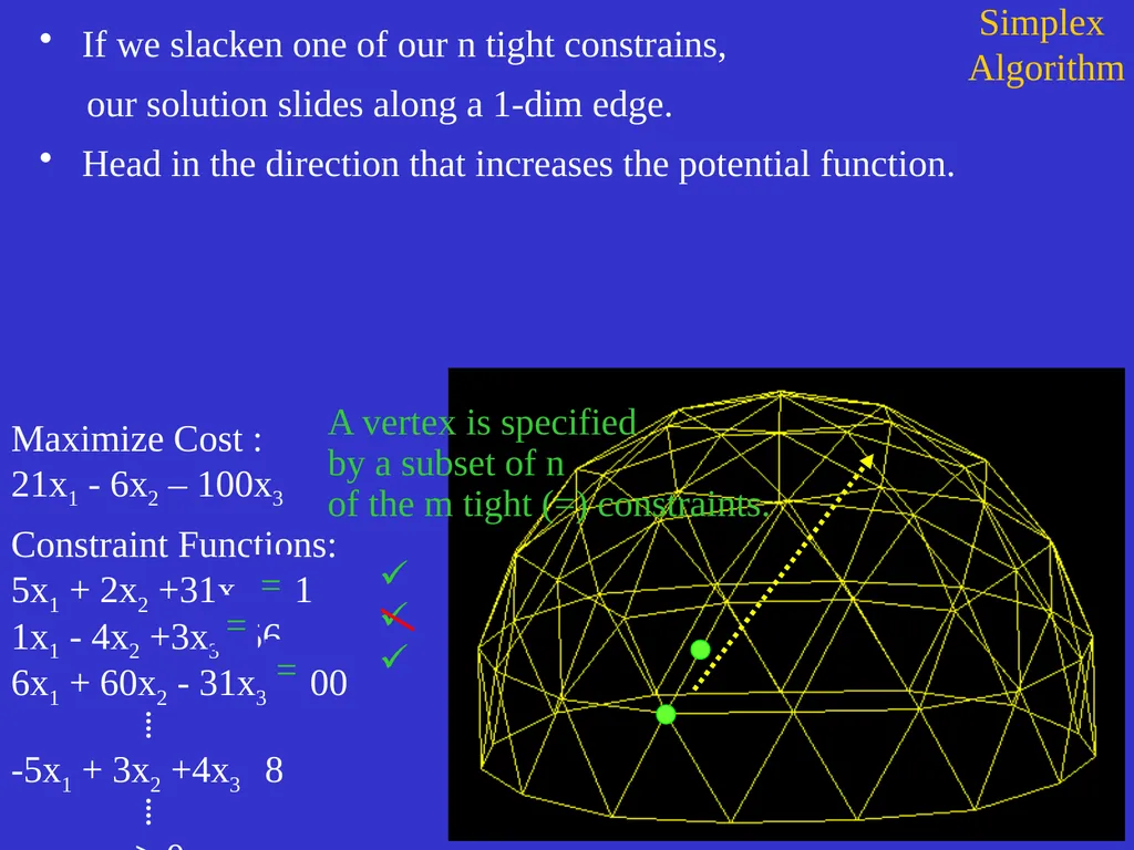
Constraint Functions:5x1 + 2x2 +31x3  211x1 - 4x2 +3x3  566x1 + 60x2 - 31x3  200 ⁞-5x1 + 3x2 +4x3  8 ⁞x1, x2, x3 ³ 0 If we slacken one of our n tight constrains,
our solution slides along a 1-dim edge.
Head in the direction that increases the potential function. Simplex Algorithm = = =<br>
slide21. Maximize Cost : 21x1 - 6x2 – 100x3
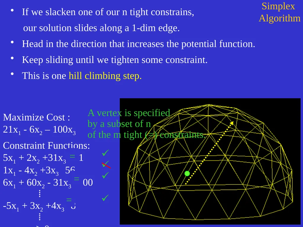
Constraint Functions:5x1 + 2x2 +31x3  211x1 - 4x2 +3x3  566x1 + 60x2 - 31x3  200 ⁞-5x1 + 3x2 +4x3  8 ⁞x1, x2, x3 ³ 0 If we slacken one of our n tight constrains,
our solution slides along a 1-dim edge.
Head in the direction that increases the potential function.
Keep sliding until we tighten some constraint.
This is one hill climbing step. Simplex Algorithm = = =<br>
slide22. Maximize Cost : 21x1 - 6x2 – 100x3
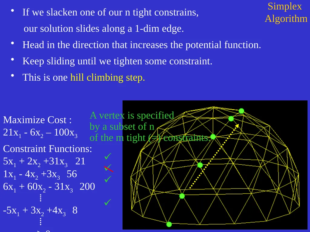
Constraint Functions:5x1 + 2x2 +31x3  211x1 - 4x2 +3x3  566x1 + 60x2 - 31x3  200 ⁞-5x1 + 3x2 +4x3  8 ⁞x1, x2, x3 ³ 0 If we slacken one of our n tight constrains,
our solution slides along a 1-dim edge.
Head in the direction that increases the potential function.
Keep sliding until we tighten some constraint.
This is one hill climbing step. Simplex Algorithm<br>
slide23. Simplex Algorithm But practically it tends to be fast. Bread and butter of optimization in industry. Maximize Cost : 21x1 - 6x2 – 100x3
Constraint Functions:5x1 + 2x2 +31x3  211x1 - 4x2 +3x3  566x1 + 60x2 - 31x3  200 ⁞-5x1 + 3x2 +4x3  8 ⁞x1, x2, x3 ³ 0<br>
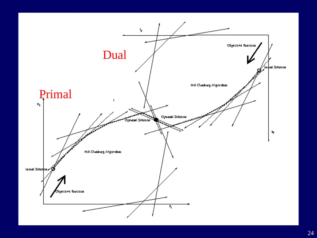
slide24. Primal Dual<br>
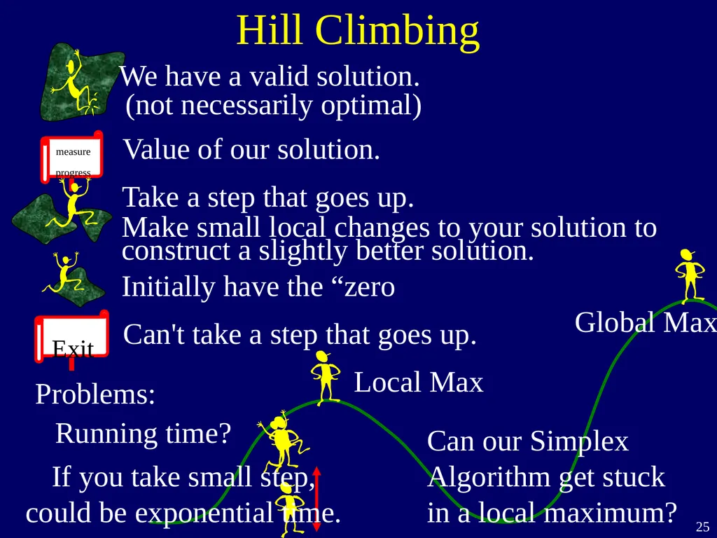
slide25. Hill Climbing We have a valid solution. (not necessarily optimal) Take a step that goes up. Value of our solution. Problems: Can't take a step that goes up. Running time? Initially have the “zero Local Max Global Max Can our SimplexAlgorithm get stuck in a local maximum? Make small local changes to your solution toconstruct a slightly better solution. If you take small step,could be exponential time.<br>
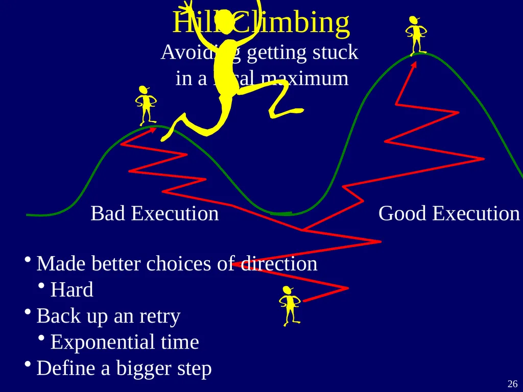
slide26. Hill Climbing Avoiding getting stuck in a local maximum Good Execution Bad Execution Made better choices of direction
Hard
Back up an retry
Exponential time
Define a bigger step<br>
slide27. Network Flow Can our Simplex Algorithm get stuck in local max? Need to prove
for every linear program
for every choice of steps
an optimal solution is found! No! How?<br>
slide28. Primal-Dual Hill Climbing<br>
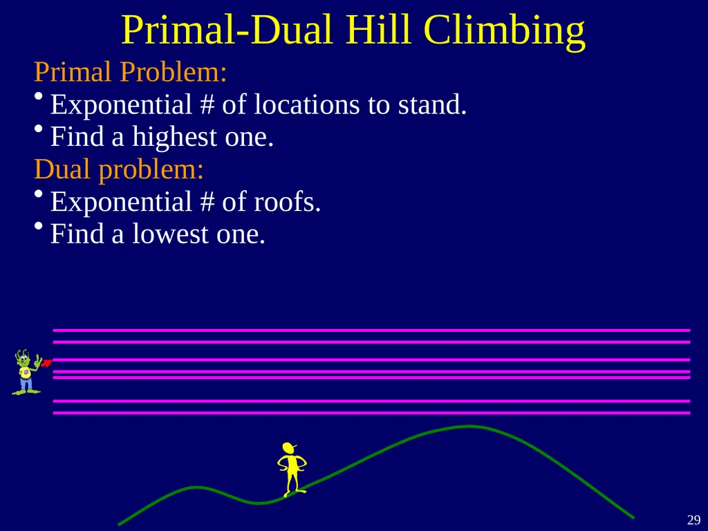
slide29. Primal-Dual Hill Climbing Primal Problem:
Exponential # of locations to stand.
Find a highest one.
Dual problem:
Exponential # of roofs.
Find a lowest one.<br>
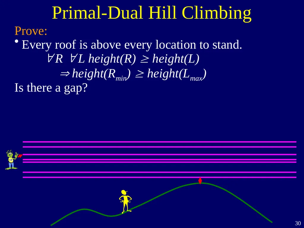
slide30. Primal-Dual Hill Climbing Prove:
Every roof is above every location to stand.
 R  L height(R)  height(L)
 height(Rmin)  height(Lmax)
Is there a gap?<br>
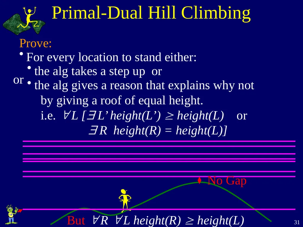
slide31. Primal-Dual Hill Climbing Prove:
For every location to stand either:
the alg takes a step up or
the alg gives a reason that explains why not by giving a roof of equal height.
i.e.  L [ L’ height(L’)  height(L) or
 R height(R) = height(L)] or But  R  L height(R)  height(L)<br>
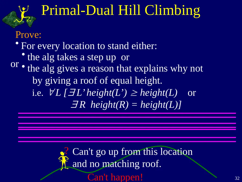
slide32. Primal-Dual Hill Climbing Prove:
For every location to stand either:
the alg takes a step up or
the alg gives a reason that explains why not by giving a roof of equal height.
i.e.  L [ L’ height(L’)  height(L) or
 R height(R) = height(L)] or Can't go up from this location and no matching roof. Can't happen! ?<br>
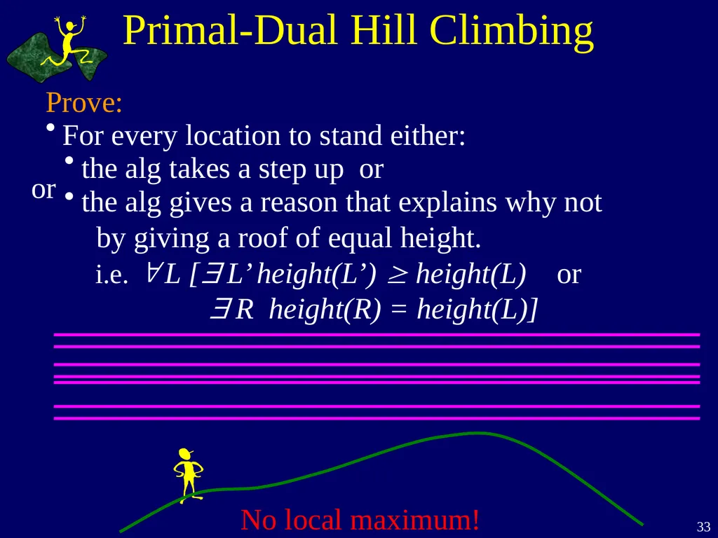
slide33. Primal-Dual Hill Climbing Prove:
For every location to stand either:
the alg takes a step up or
the alg gives a reason that explains why not by giving a roof of equal height.
i.e.  L [ L’ height(L’)  height(L) or
 R height(R) = height(L)] or<br>
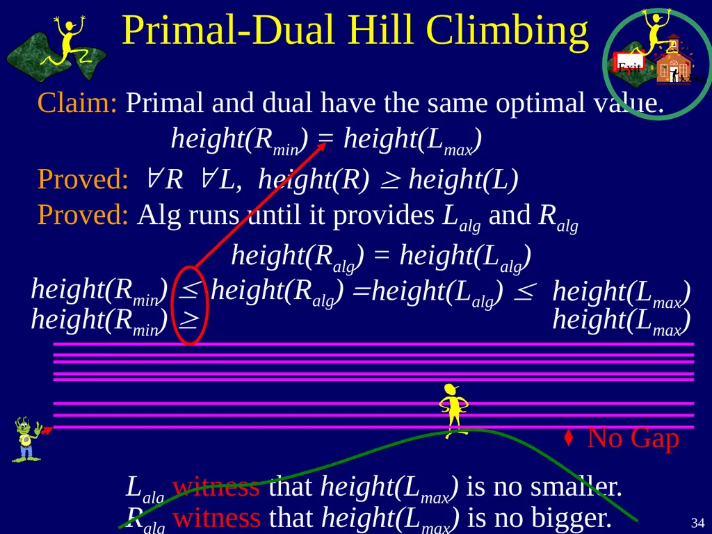
slide34. Primal-Dual Hill Climbing Claim: Primal and dual have the same optimal value. height(Rmin) = height(Lmax)
Proved:  R  L, height(R)  height(L)
Proved: Alg runs until it provides Lalg and Ralg height(Ralg) = height(Lalg) height(Rmin)  height(Ralg) = height(Lalg)  height(Lmax) height(Rmin)  height(Lmax) Lalg witness that height(Lmax) is no smaller. Ralg witness that height(Lmax) is no bigger.<br>
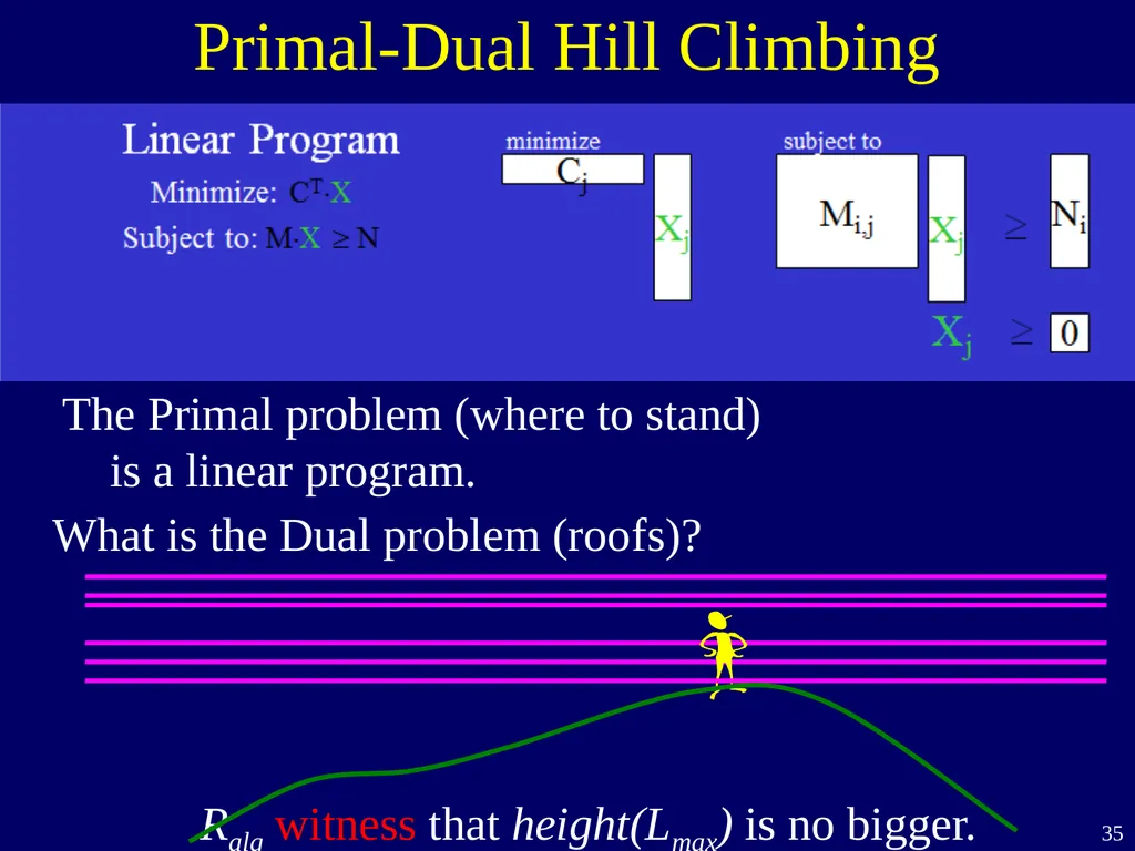
slide35. Primal-Dual Hill Climbing Ralg witness that height(Lmax) is no bigger. The Primal problem (where to stand)  is a linear program. What is the Dual problem (roofs)?<br>
slide36. Linear Program
Minimize: CTX
Subject to: MX ³ N n variable xj that we are looking for values of.
An optimization function
Each has a variable has a coefficient cj.
The dot product CTX gives one value to minimize.
m constraints:
Some linear combination of the variablesmust be at least some set value.
i MiX ³ Ni
Generally implied that variables are positive. Duality<br>
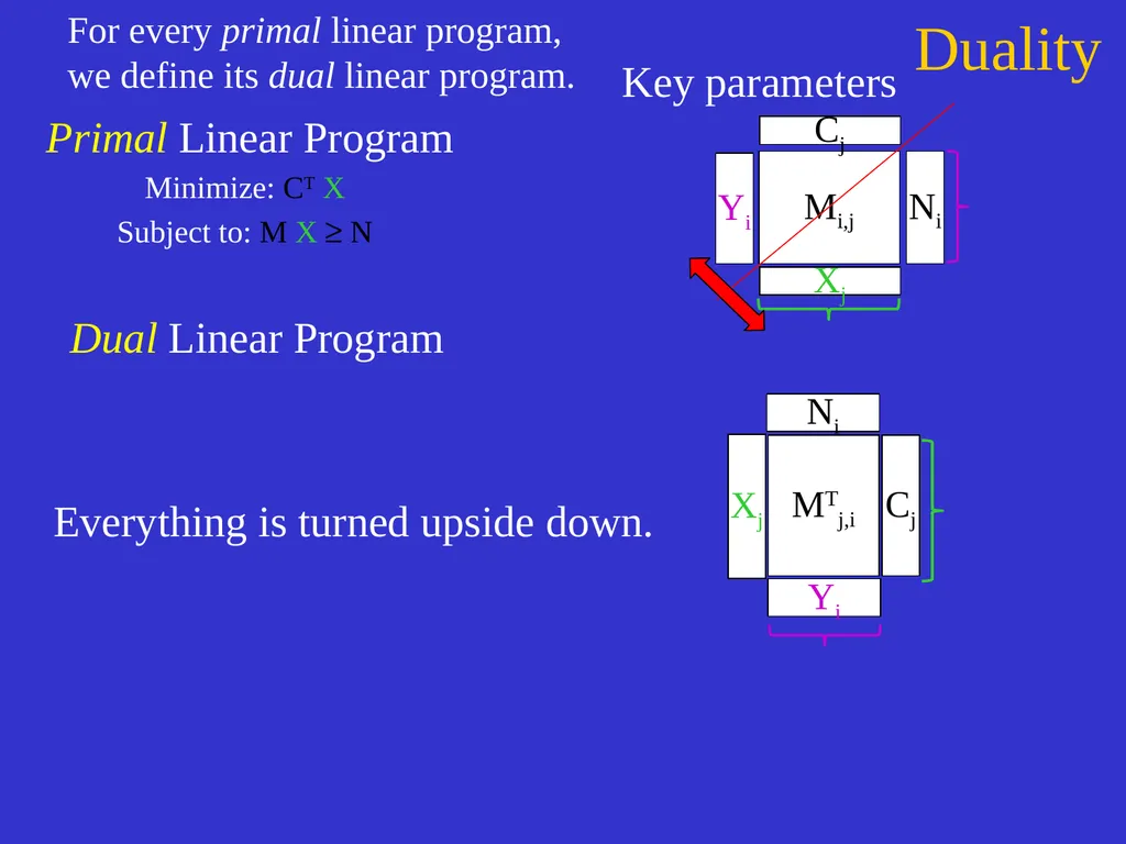
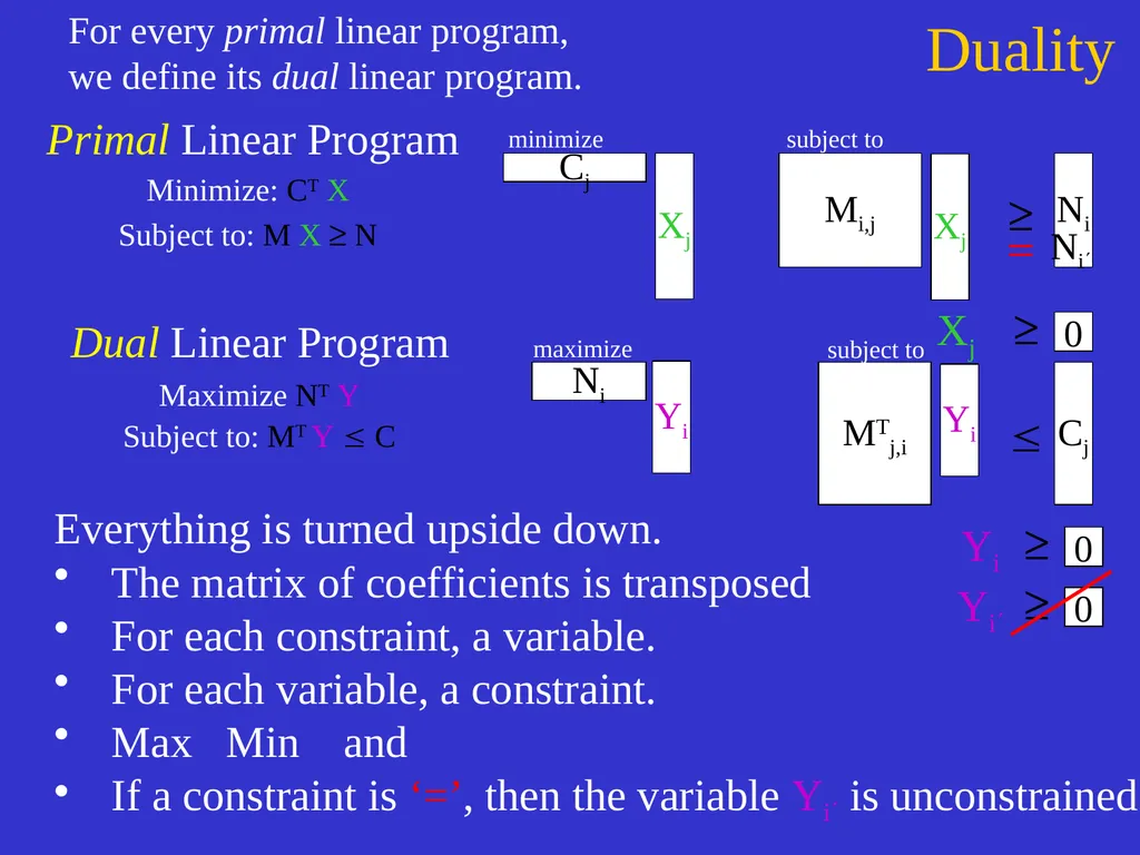
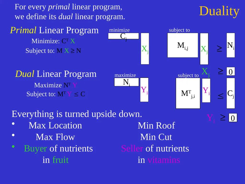
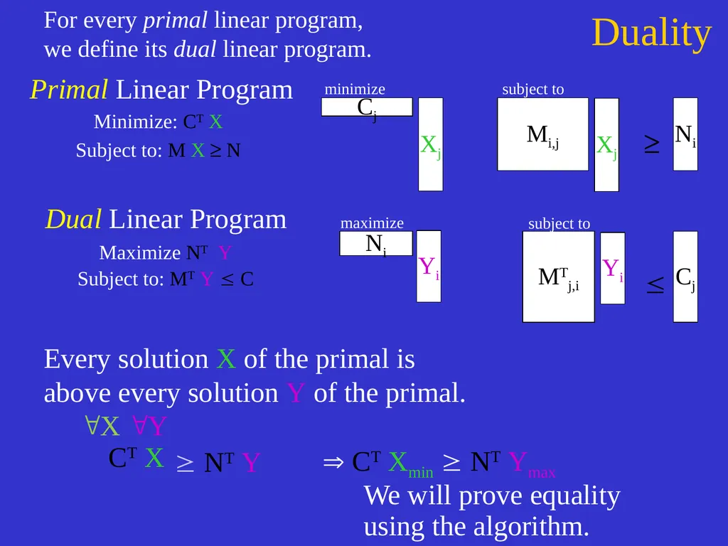
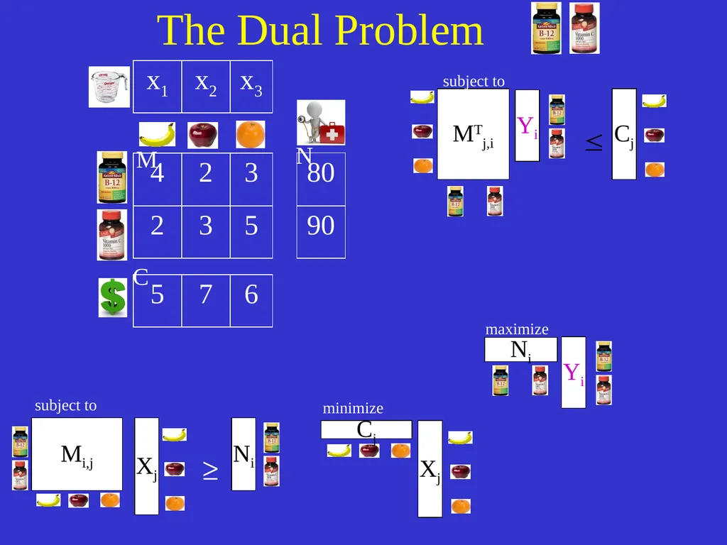
slide37. Duality Dual Linear Program For every primal linear program, we define its dual linear program. Everything is turned upside down. Primal Linear Program
Minimize: CTX
Subject to: MX ³ N Yi<br>
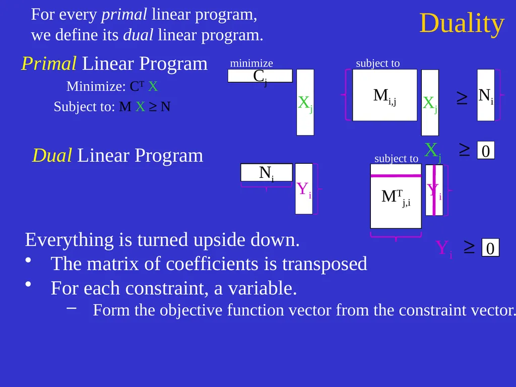
slide38. Duality Dual Linear Program Ni For every primal linear program, we define its dual linear program. Everything is turned upside down.
The matrix of coefficients is transposed
For each constraint, a variable.
Form the objective function vector from the constraint vector. Mi,j Xj Ni ³ subject to Primal Linear Program
Minimize: CTX
Subject to: MX ³ N Xj Cj minimize<br>
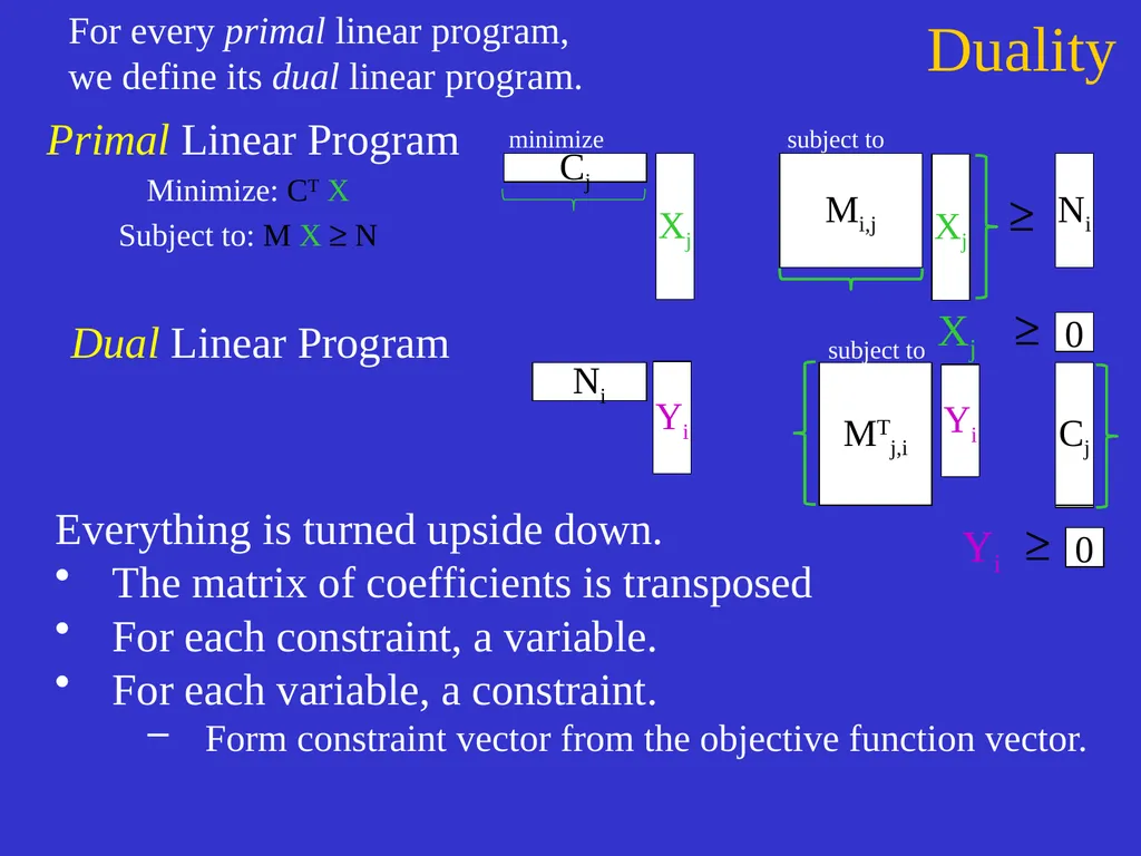
slide39. Duality Dual Linear Program Ni Cj For every primal linear program, we define its dual linear program. Everything is turned upside down.
The matrix of coefficients is transposed
For each constraint, a variable.
For each variable, a constraint.
Form constraint vector from the objective function vector. Yi Mi,j Xj Ni ³ subject to Primal Linear Program
Minimize: CTX
Subject to: MX ³ N Xj Cj minimize Yi<br>
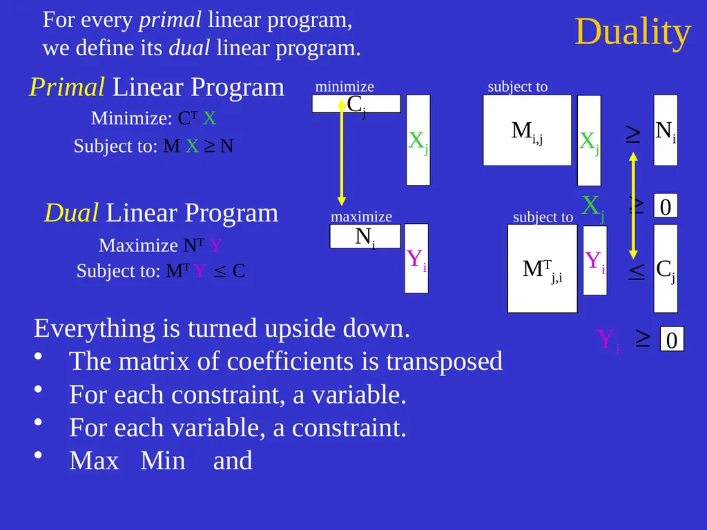
slide40. Duality Dual Linear Program Ni Cj  For every primal linear program, we define its dual linear program. Everything is turned upside down.
The matrix of coefficients is transposed
For each constraint, a variable.
For each variable, a constraint.
Max  Min and    Maximize NT Y
Subject to: MT Y  C maximize Yi Mi,j Xj Ni ³ subject to Primal Linear Program
Minimize: CTX
Subject to: MX ³ N Xj Cj minimize Yi<br>
slide41. Duality Dual Linear Program Ni Cj For every primal linear program, we define its dual linear program. Everything is turned upside down.
The matrix of coefficients is transposed
For each constraint, a variable.
For each variable, a constraint.
Max  Min and   
If a constraint is ‘=’, then the variable Yi is unconstrained. maximize Yi Mi,j Xj Ni subject to Primal Linear Program
Minimize: CTX
Subject to: MX ³ N Xj Cj minimize Yi  ³ Maximize NT Y
Subject to: MT Y  C<br>
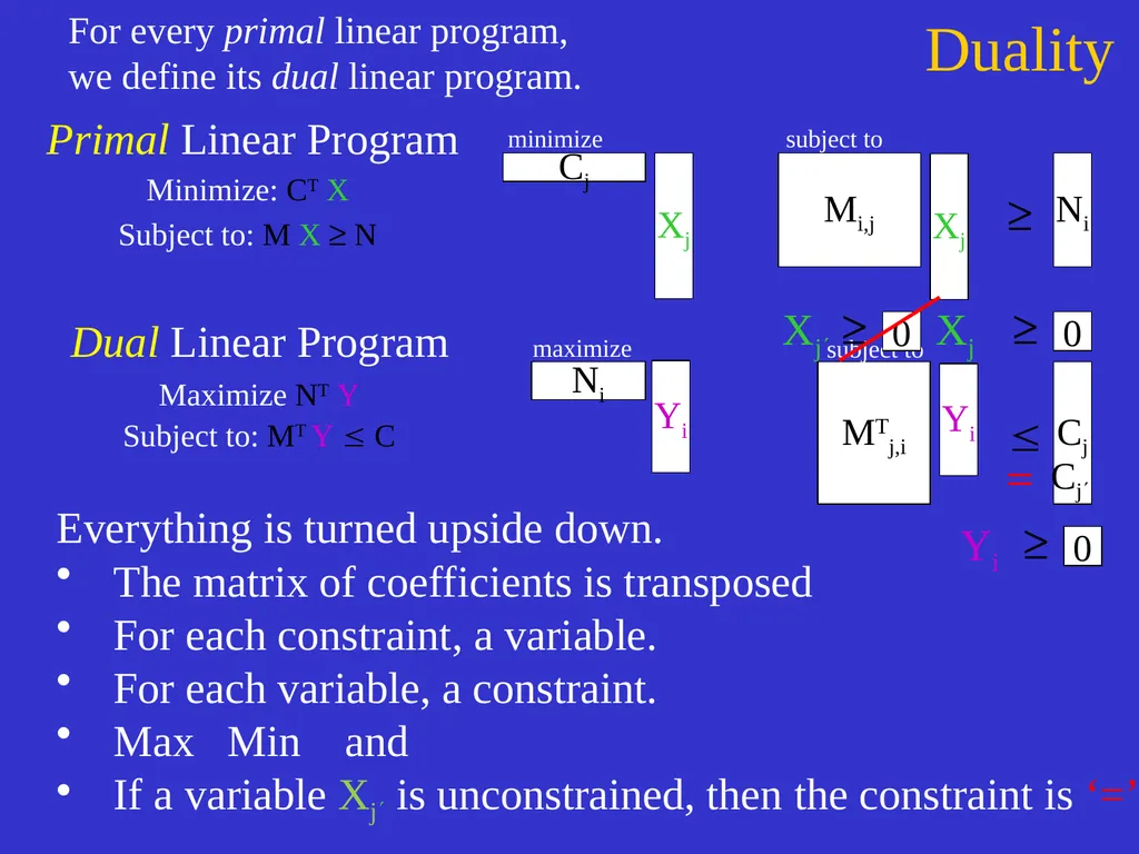
slide42. Duality Dual Linear Program Ni Cj For every primal linear program, we define its dual linear program. Everything is turned upside down.
The matrix of coefficients is transposed
For each constraint, a variable.
For each variable, a constraint.
Max  Min and   
If a variable Xj is unconstrained, then the constraint is ‘=’. maximize Yi Mi,j Xj Ni subject to Primal Linear Program
Minimize: CTX
Subject to: MX ³ N Xj Cj minimize Yi ³  Maximize NT Y
Subject to: MT Y  C<br>
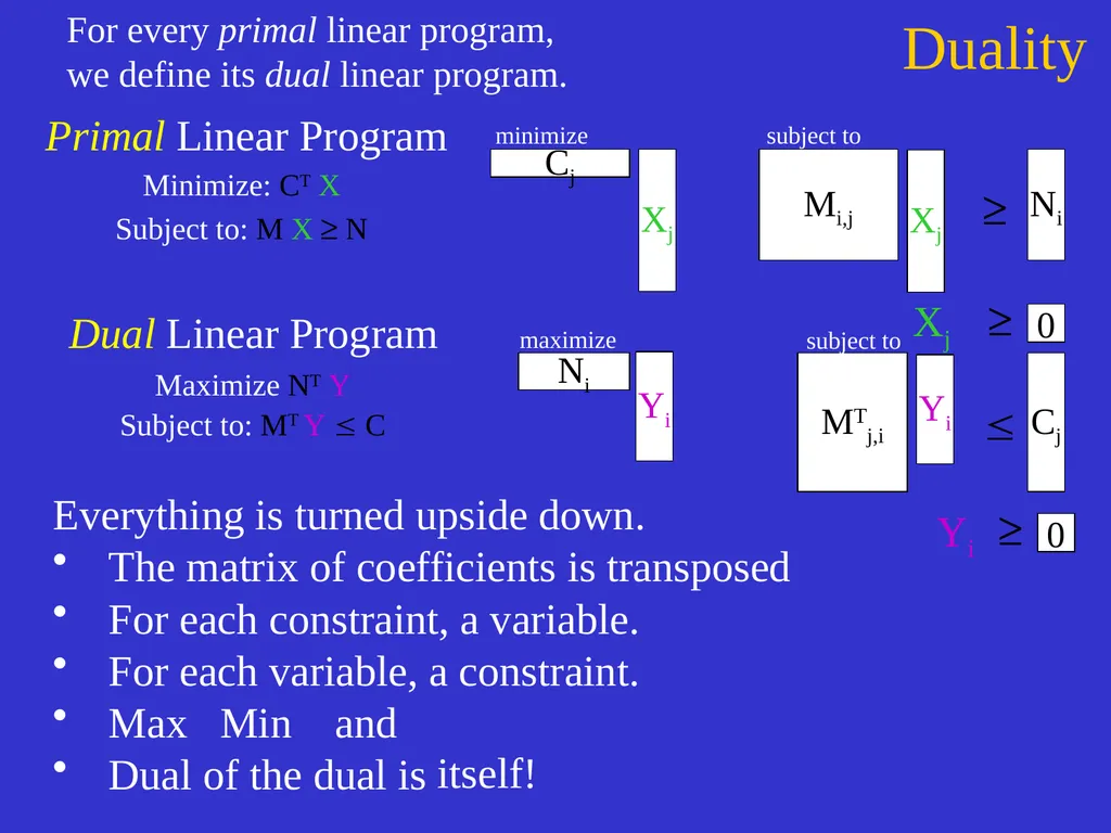
slide43. Duality Dual Linear Program Ni Cj For every primal linear program, we define its dual linear program. Everything is turned upside down.
The matrix of coefficients is transposed
For each constraint, a variable.
For each variable, a constraint.
Max  Min and   
Dual of the dual is ? maximize Yi Mi,j Xj Ni subject to Primal Linear Program
Minimize: CTX
Subject to: MX ³ N Xj Cj minimize Yi ³  Maximize NT Y
Subject to: MT Y  C itself!<br>
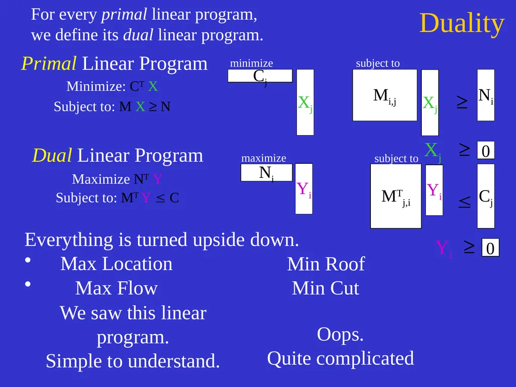
slide44. Duality Dual Linear Program Ni Cj  For every primal linear program, we define its dual linear program. maximize Yi Mi,j Xj Ni ³ subject to Primal Linear Program
Minimize: CTX
Subject to: MX ³ N Xj Cj minimize Yi Everything is turned upside down.
Max Location 
Max Flow  Maximize NT Y
Subject to: MT Y  C Min Roof
Min Cut Oops.Quite complicated We saw this linear program.Simple to understand.<br>
slide45. Duality Dual Linear Program Ni Cj  For every primal linear program, we define its dual linear program. maximize Yi Mi,j Xj Ni ³ subject to Primal Linear Program
Minimize: CTX
Subject to: MX ³ N Xj Cj minimize Yi Everything is turned upside down.
Max Location 
Max Flow 
Buyer of nutrients 
in fruit Maximize NT Y
Subject to: MT Y  C Min Roof
Min Cut
Seller of nutrients
in vitamins<br>
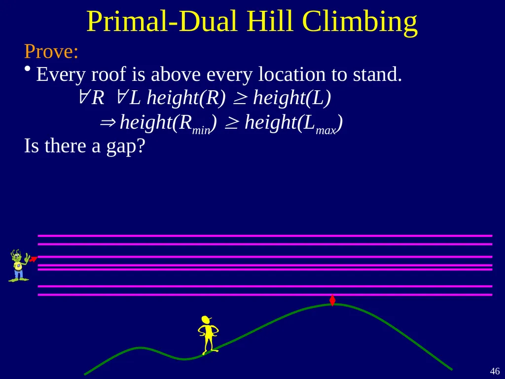
slide46. Primal-Dual Hill Climbing Prove:
Every roof is above every location to stand.
 R  L height(R)  height(L)
 height(Rmin)  height(Lmax)
Is there a gap?<br>
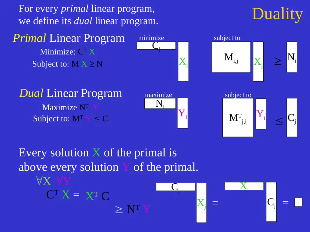
slide47. Duality Dual Linear Program Ni Cj  For every primal linear program, we define its dual linear program. maximize Yi Mi,j Xj Ni ³ subject to Primal Linear Program
Minimize: CTX
Subject to: MX ³ N Xj Cj minimize Yi Every solution X of the primal is above every solution Y of the primal.
X Y
CTX = Maximize NT Y
Subject to: MTY  C XTC  NTY<br>
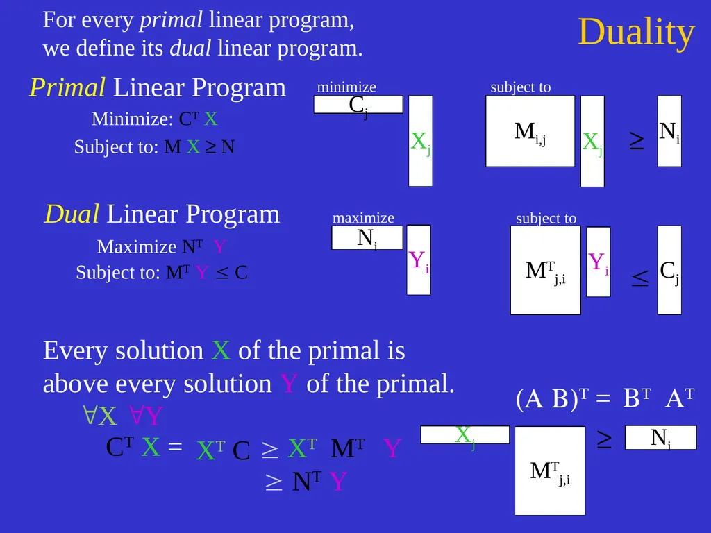
slide48. Duality Dual Linear Program Ni Cj  For every primal linear program, we define its dual linear program. maximize Yi Mi,j Xj Ni ³ subject to Primal Linear Program
Minimize: CTX
Subject to: MX ³ N Xj Cj minimize Yi Every solution X of the primal is above every solution Y of the primal.
X Y
CTX =  NTY XTC  XT MT  Y Maximize NT Y
Subject to: MTY  C (AB)T = BT AT<br>
slide49. Duality Dual Linear Program Ni Cj  For every primal linear program, we define its dual linear program. maximize Yi Mi,j Xj Ni ³ subject to Primal Linear Program
Minimize: CTX
Subject to: MX ³ N Xj Cj minimize Yi Every solution X of the primal is above every solution Y of the primal.
X Y
CTX  NTY Maximize NT Y
Subject to: MTY  C  CTXmin  NTYmax We will prove equality
using the algorithm.<br>
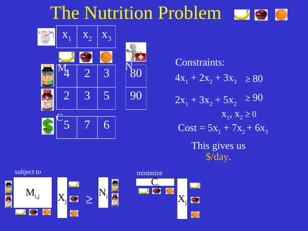
slide50. The Nutrition Problem An apple a day keeps the doctor away – but apples are costly! A customer’s goal isto fulfill daily vitamin requirements at lowest cost.<br>
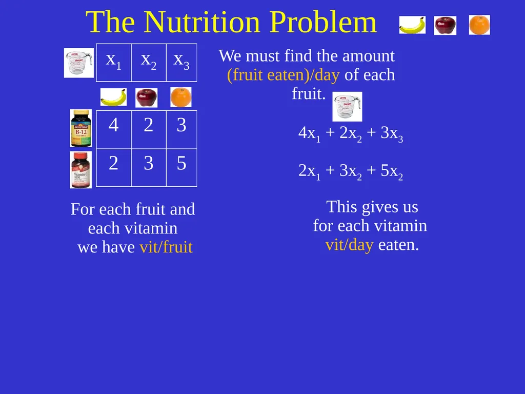
slide51. The Nutrition Problem 4x1 + 2x2 + 3x3
2x1 + 3x2 + 5x2 We must find the amount  (fruit eaten)/day of each fruit. For each fruit and each vitamin we have vit/fruit This gives usfor each vitamin vit/day eaten.<br>
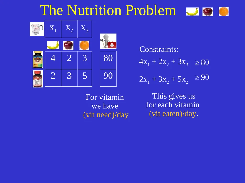
slide52. The Nutrition Problem 4x1 + 2x2 + 3x3
2x1 + 3x2 + 5x2 For vitamin we have (vit need)/day ³ 80

³ 90 This gives usfor each vitamin (vit eaten)/day. Constraints:<br>
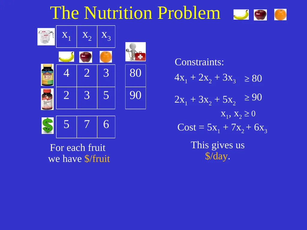
slide53. The Nutrition Problem 4x1 + 2x2 + 3x3
2x1 + 3x2 + 5x2 ³ 80

³ 90 Constraints: x1, x2 ³ 0 Cost = 5x1 + 7x2 + 6x3 For each fruit we have $/fruit This gives us$/day.<br>
slide54. The Nutrition Problem 4x1 + 2x2 + 3x3
2x1 + 3x2 + 5x2 ³ 80

³ 90 Constraints: x1, x2 ³ 0 Cost = 5x1 + 7x2 + 6x3 This gives us$/day.<br>
slide55. The Dual Problem<br>
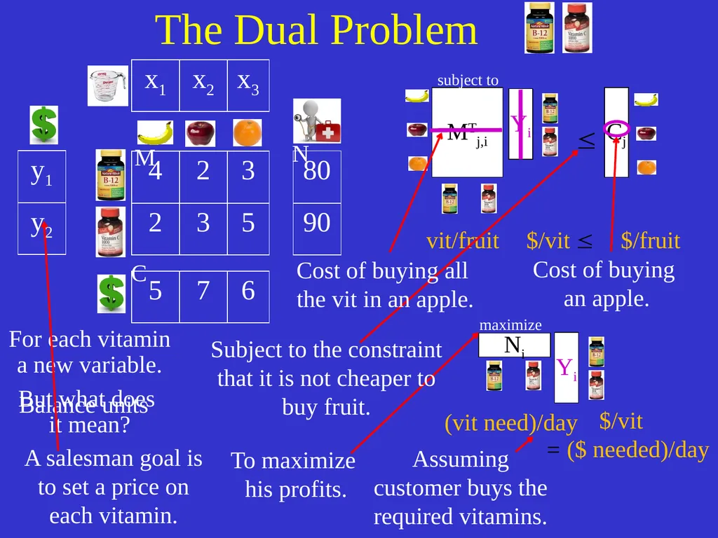
slide56. The Dual Problem For each vitamina new variable. But what does it mean? M N C (vit need)/day vit/fruit $/fruit $/vit ($ needed)/day $/vit =  Balance units<br>
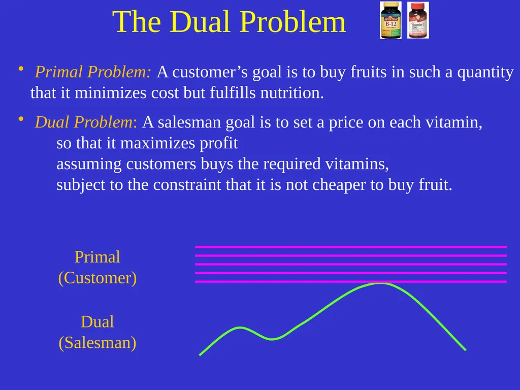
slide57. Primal Problem: A customer’s goal is to buy fruits in such a quantity that it minimizes cost but fulfills nutrition.
Dual Problem: A salesman goal is to set a price on each vitamin,  so that it maximizes profit  assuming customers buys the required vitamins, subject to the constraint that it is not cheaper to buy fruit. Primal (Customer) Dual (Salesman) The Dual Problem<br>
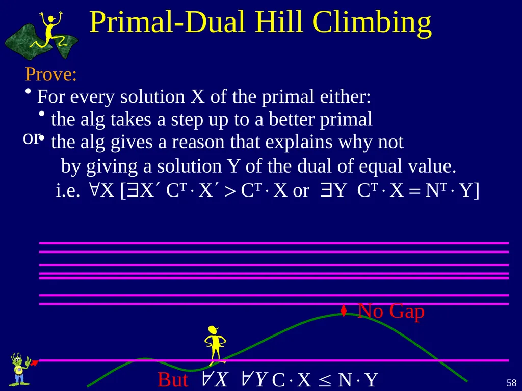
slide58. Primal-Dual Hill Climbing Prove:
For every solution X of the primal either:
the alg takes a step up to a better primal
the alg gives a reason that explains why not by giving a solution Y of the dual of equal value.
i.e. X [X CTX > CTX or Y CTX = NTY] or But  X  Y CX  NY<br>
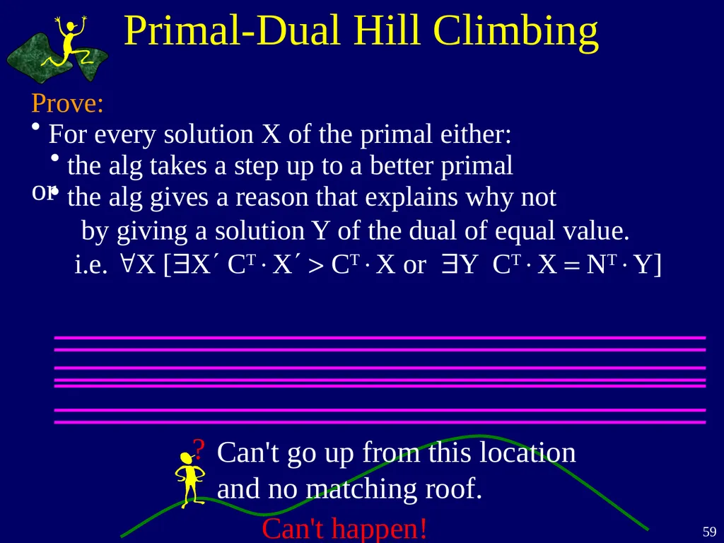
slide59. Primal-Dual Hill Climbing or Can't go up from this location and no matching roof. Can't happen! ? Prove:
For every solution X of the primal either:
the alg takes a step up to a better primal
the alg gives a reason that explains why not by giving a solution Y of the dual of equal value.
i.e. X [X CTX > CTX or Y CTX = NTY]<br>
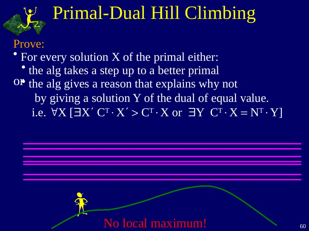
slide60. Primal-Dual Hill Climbing or Prove:
For every solution X of the primal either:
the alg takes a step up to a better primal
the alg gives a reason that explains why not by giving a solution Y of the dual of equal value.
i.e. X [X CTX > CTX or Y CTX = NTY]<br>
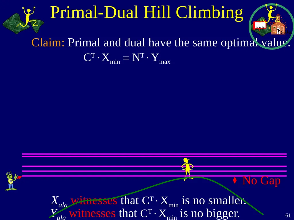
slide61. Primal-Dual Hill Climbing Claim: Primal and dual have the same optimal value. CTXmin = NTYmax Xalg witnesses that CTXmin is no smaller. Yalg witnesses that CTXmin is no bigger.<br>
slide62. Maximize Cost : 21x1 - 6x2 – 7x3
Constraint Functions: 5x1 + 2x2 + 9x3  21 1x1 - 4x2 + 3x3  56 6x1 + 6x2 - 8x3  78 ⁞
-5x1 + 3x2 +4x3  8 ⁞
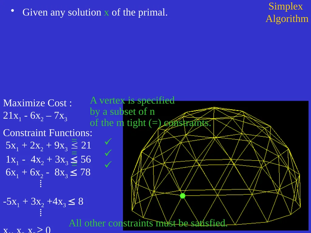
x1, x2, x3 ³ 0 Given any solution x of the primal. Simplex Algorithm All other constraints must be satisfied.<br>
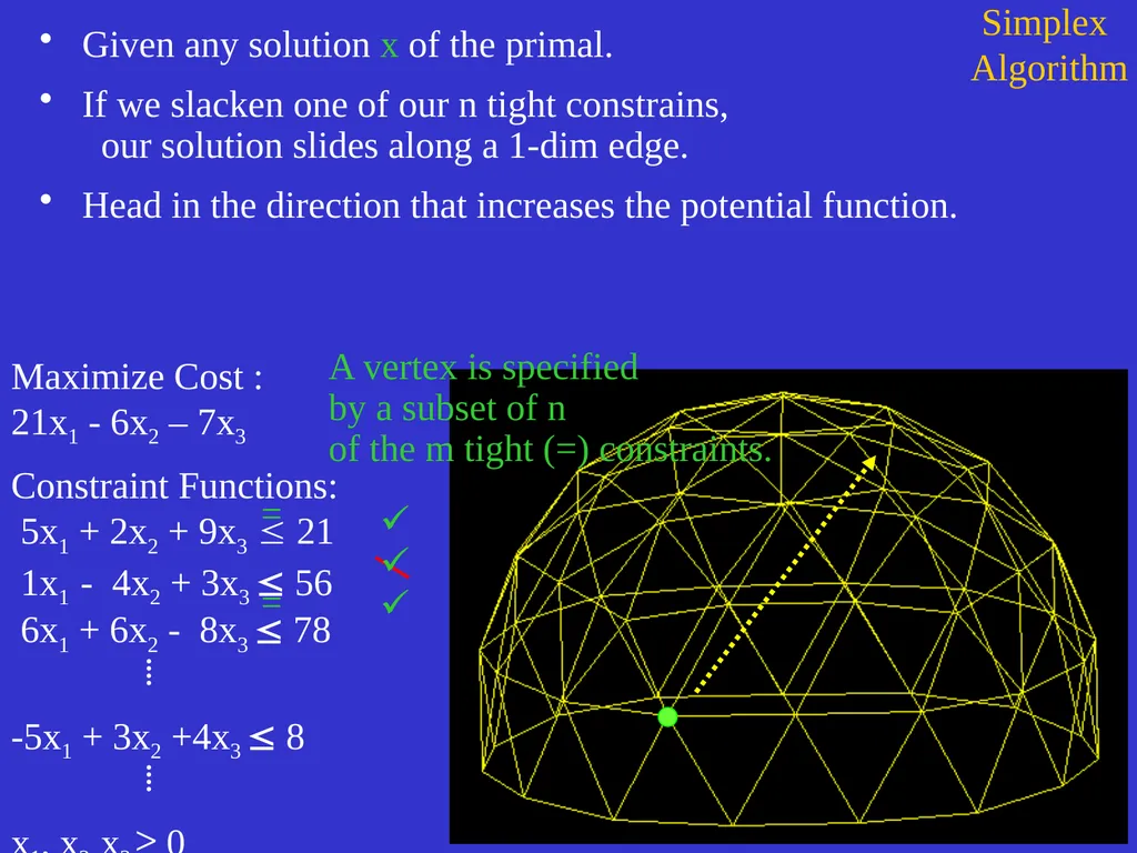
slide63. Given any solution x of the primal.
If we slacken one of our n tight constrains, our solution slides along a 1-dim edge.
Head in the direction that increases the potential function. Simplex Algorithm Maximize Cost : 21x1 - 6x2 – 7x3
Constraint Functions: 5x1 + 2x2 + 9x3  21 1x1 - 4x2 + 3x3  56 6x1 + 6x2 - 8x3  78 ⁞
-5x1 + 3x2 +4x3  8 ⁞
x1, x2, x3 ³ 0<br>
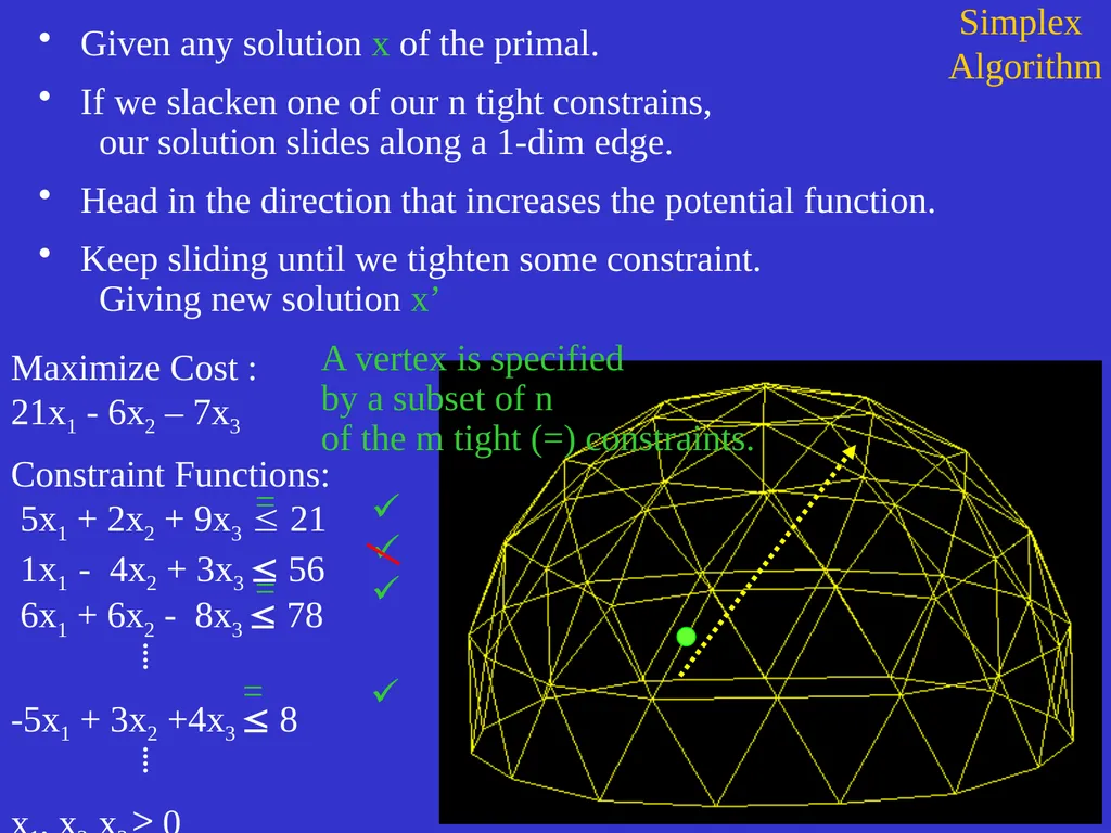
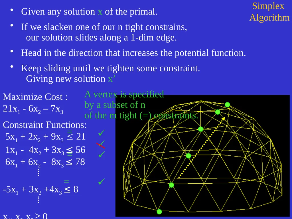
slide64. Given any solution x of the primal.
If we slacken one of our n tight constrains, our solution slides along a 1-dim edge.
Head in the direction that increases the potential function.
Keep sliding until we tighten some constraint.  Giving new solution x’ Simplex Algorithm Maximize Cost : 21x1 - 6x2 – 7x3
Constraint Functions: 5x1 + 2x2 + 9x3  21 1x1 - 4x2 + 3x3  56 6x1 + 6x2 - 8x3  78 ⁞
-5x1 + 3x2 +4x3  8 ⁞
x1, x2, x3 ³ 0 =<br>
slide65. Simplex Algorithm Maximize Cost : 21x1 - 6x2 – 7x3
Constraint Functions: 5x1 + 2x2 + 9x3  21 1x1 - 4x2 + 3x3  56 6x1 + 6x2 - 8x3  78 ⁞
-5x1 + 3x2 +4x3  8 ⁞
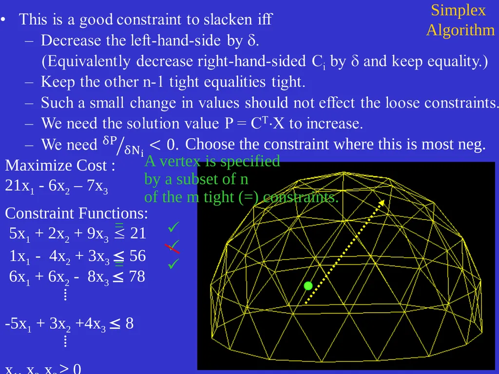
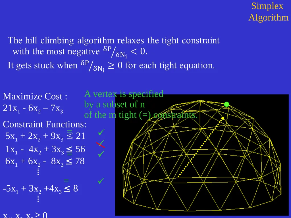
x1, x2, x3 ³ 0 Choose the constraint where this is most neg.<br>
slide66. Simplex Algorithm Given any solution x of the primal.
If we slacken one of our n tight constrains, our solution slides along a 1-dim edge.
Head in the direction that increases the potential function.
Keep sliding until we tighten some constraint.  Giving new solution x’ Maximize Cost : 21x1 - 6x2 – 7x3
Constraint Functions: 5x1 + 2x2 + 9x3  21 1x1 - 4x2 + 3x3  56 6x1 + 6x2 - 8x3  78 ⁞
-5x1 + 3x2 +4x3  8 ⁞
x1, x2, x3 ³ 0 =<br>
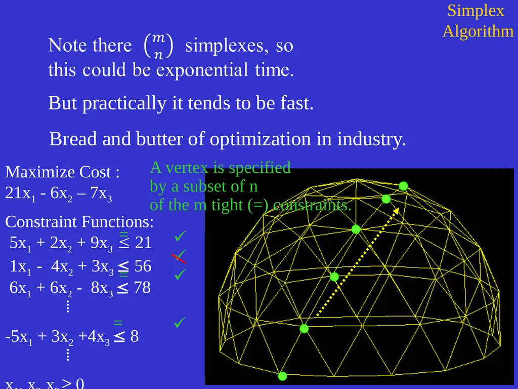
slide67. Simplex Algorithm But practically it tends to be fast. Bread and butter of optimization in industry. Maximize Cost : 21x1 - 6x2 – 7x3
Constraint Functions: 5x1 + 2x2 + 9x3  21 1x1 - 4x2 + 3x3  56 6x1 + 6x2 - 8x3  78 ⁞
-5x1 + 3x2 +4x3  8 ⁞
x1, x2, x3 ³ 0 =<br>
slide68. Simplex Algorithm Maximize Cost : 21x1 - 6x2 – 7x3
Constraint Functions: 5x1 + 2x2 + 9x3  21 1x1 - 4x2 + 3x3  56 6x1 + 6x2 - 8x3  78 ⁞
-5x1 + 3x2 +4x3  8 ⁞
x1, x2, x3 ³ 0 =<br>
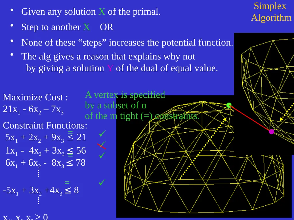
slide69. Simplex Algorithm Given any solution X of the primal.
Step to another X OR
None of these “steps” increases the potential function.
The alg gives a reason that explains why not by giving a solution Y of the dual of equal value. Maximize Cost : 21x1 - 6x2 – 7x3
Constraint Functions: 5x1 + 2x2 + 9x3  21 1x1 - 4x2 + 3x3  56 6x1 + 6x2 - 8x3  78 ⁞
-5x1 + 3x2 +4x3  8 ⁞
x1, x2, x3 ³ 0 =<br>
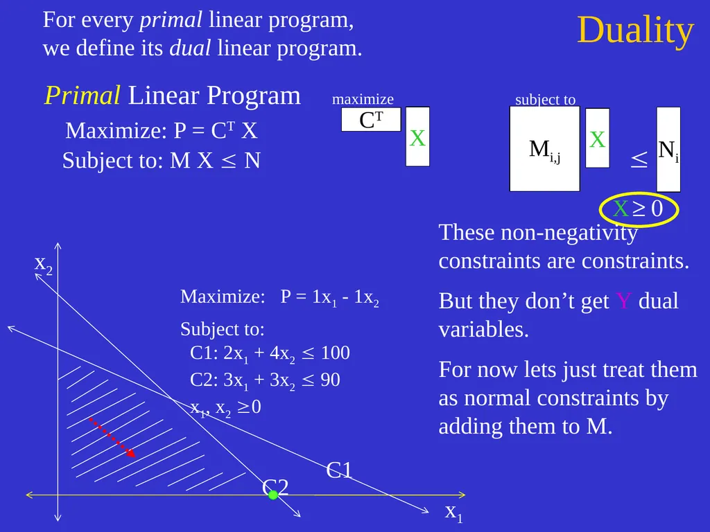
slide70. Duality These non-negativity constraints are constraints.
But they don’t get Y dual variables.
For now lets just treat themas normal constraints byadding them to M.<br>
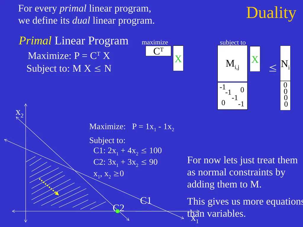
slide71. Duality For now lets just treat themas normal constraints byadding them to M.
This gives us more equations than variables.<br>
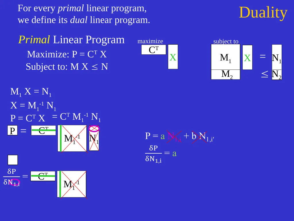
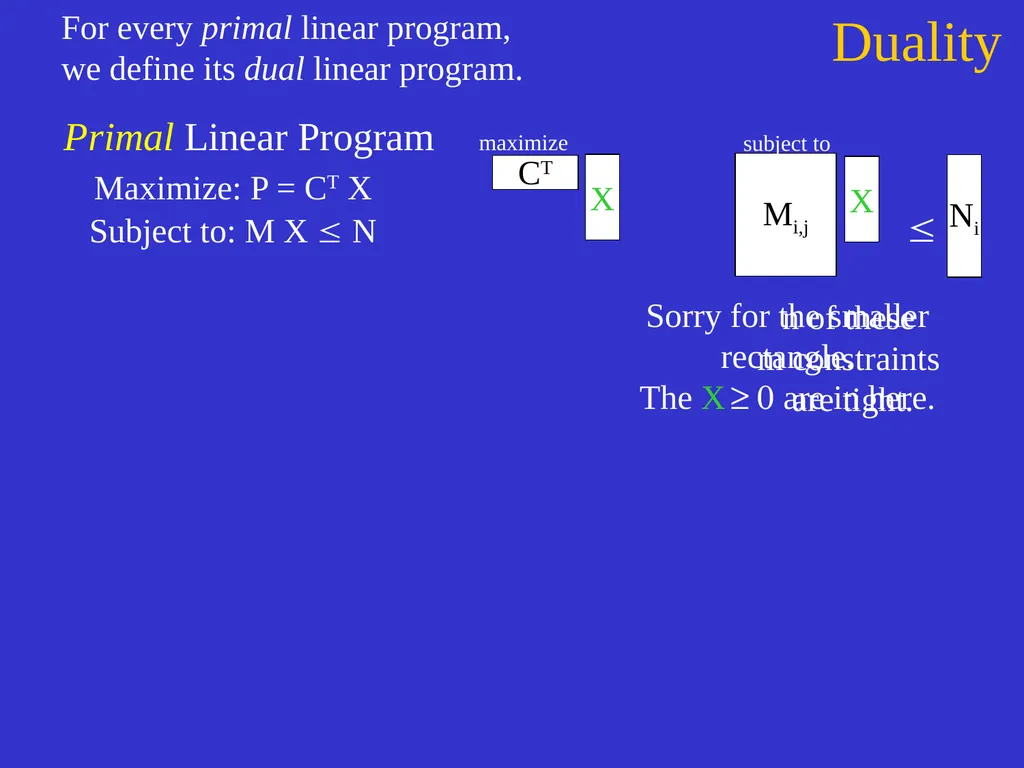
slide72. Duality Primal Linear Program Ni  For every primal linear program, we define its dual linear program. maximize Maximize: P = CTX
Subject to: MX  N n of these m constraints are tight. X X CT Sorry for the smaller rectangle.The X ³ 0 are in here.<br>
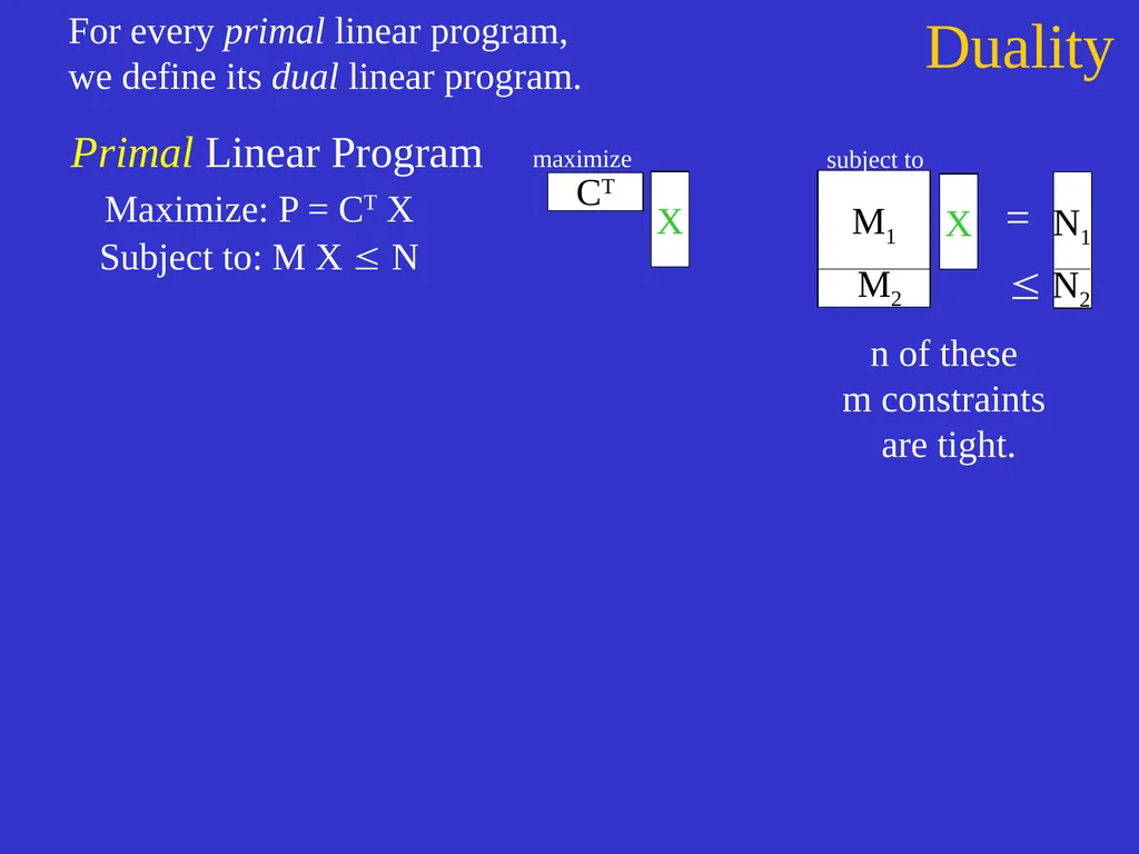
slide73. Duality Primal Linear Program For every primal linear program, we define its dual linear program. maximize X Maximize: P = CTX
Subject to: MX  N n of these m constraints are tight. X CT<br>
slide74. Duality Primal Linear Program For every primal linear program, we define its dual linear program. maximize X Maximize: P = CTX
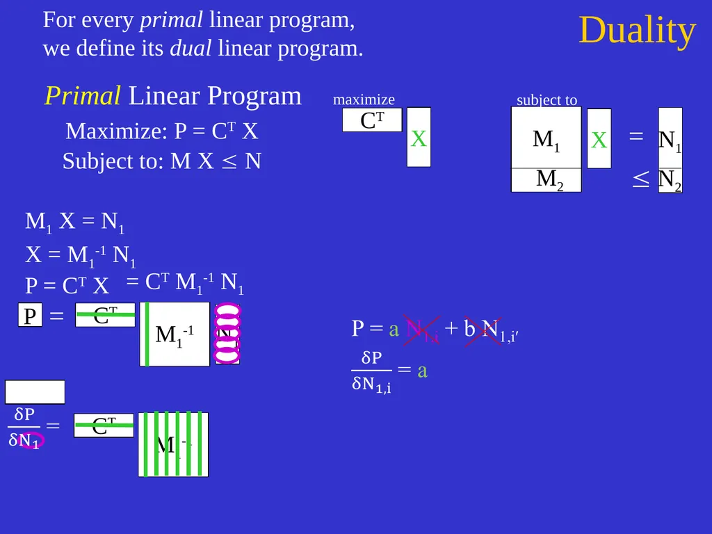
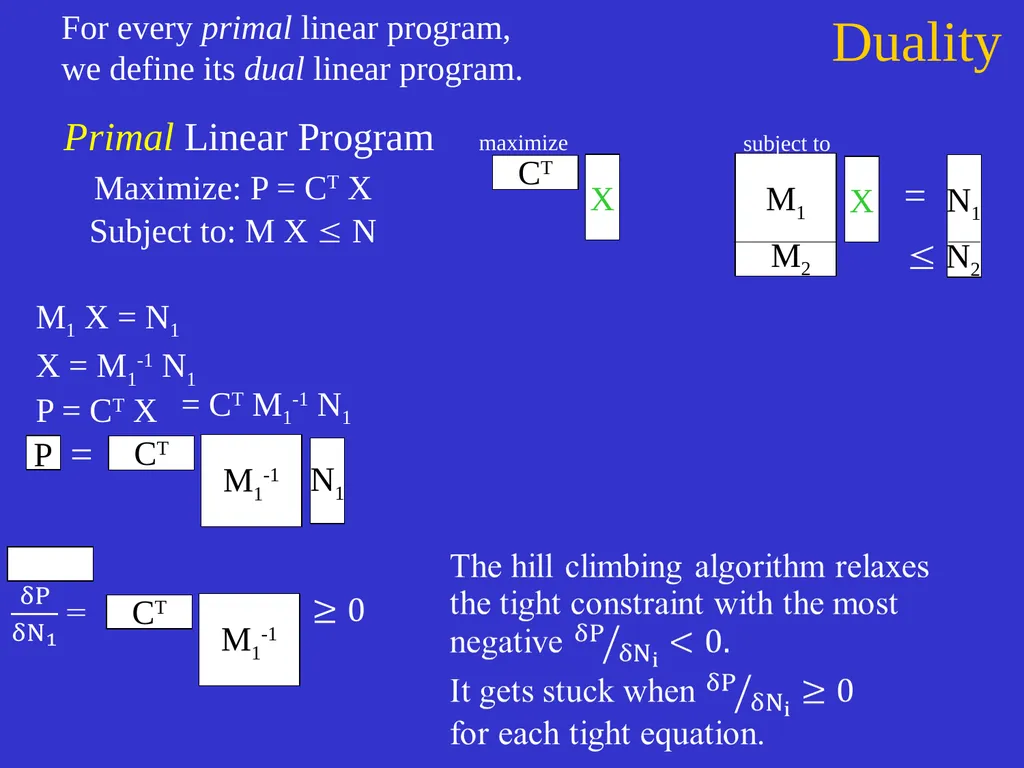
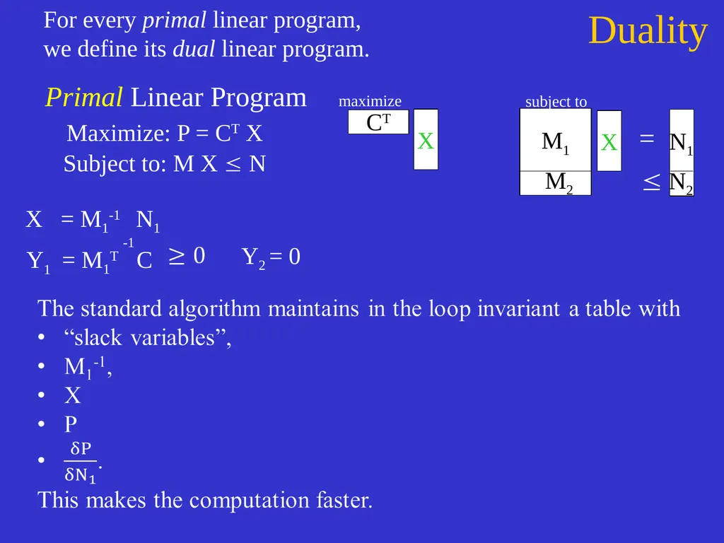
Subject to: MX  N M1X = N1
X = M1-1N1
P = CTX = CTM1-1N1 X CT<br>
slide75. Duality Primal Linear Program For every primal linear program, we define its dual linear program. maximize X Maximize: P = CTX
Subject to: MX  N M1X = N1
X = M1-1N1
P = CTX = CTM1-1N1 X CT<br>
slide76. Duality Primal Linear Program For every primal linear program, we define its dual linear program. maximize X Maximize: P = CTX
Subject to: MX  N M1X = N1
X = M1-1N1
P = CTX = CTM1-1N1 X CT<br>
slide77. Duality Primal Linear Program For every primal linear program, we define its dual linear program. maximize X Maximize: P = CTX
Subject to: MX  N M1X = N1
X = M1-1N1
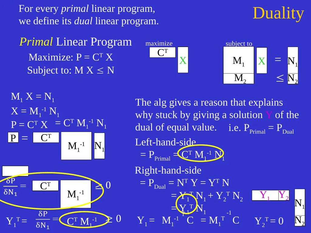
P = CTX = CTM1-1N1 X CT The alg gives a reason that explains why stuck by giving a solution Y of the dual of equal value. Left-hand-side
= PPrimal = CTM1-1N1 Right-hand-side = PDual = NTY = YTN
= Y1TN1 + Y2TN2
= Y1TN1 Y2T = 0 Y1T = CTM1-1 i.e. PPrimal = PDual Y1 =<br>
slide78. Duality Primal Linear Program For every primal linear program, we define its dual linear program. maximize X Maximize: P = CTX
Subject to: MX  N X CT Left-hand-side
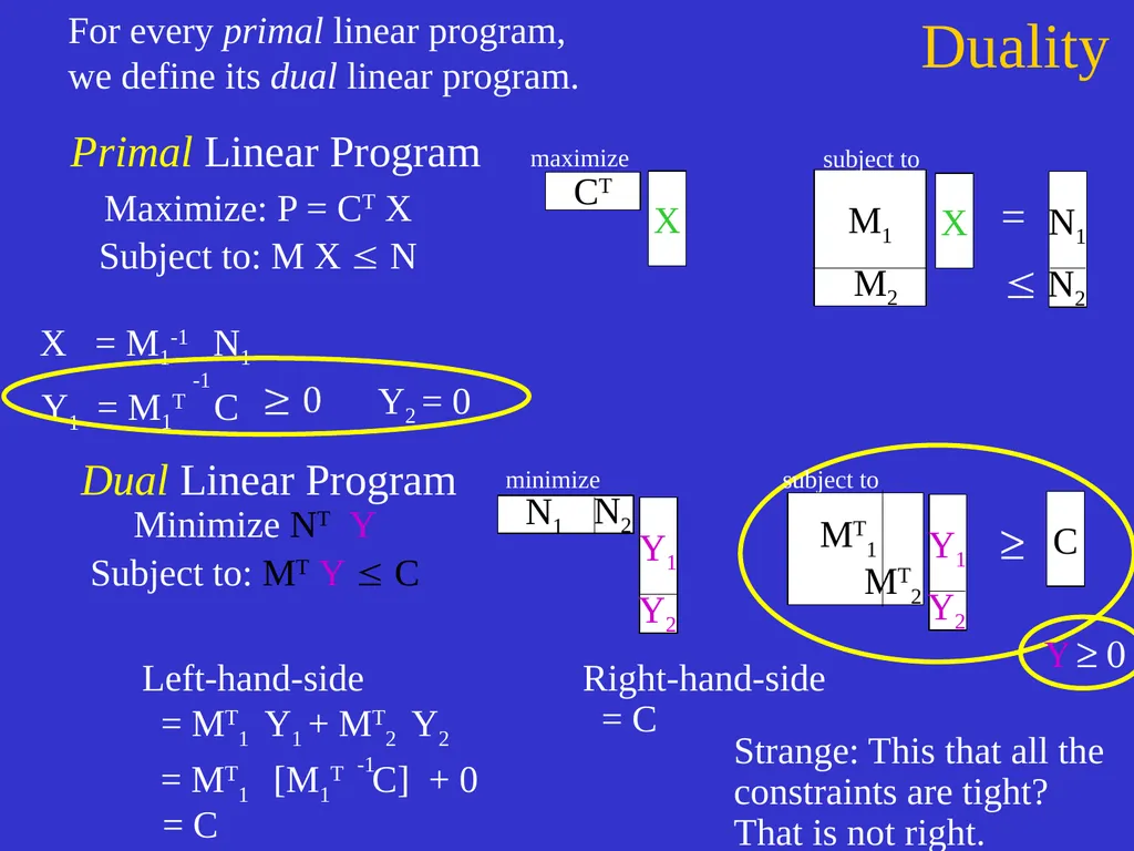
= MT1 Y1 + MT2 Y2 Right-hand-side = C = C Strange: This that all the constraints are tight? That is not right.<br>
slide79. Duality Primal Linear Program For every primal linear program, we define its dual linear program. maximize X Maximize: P = CTX
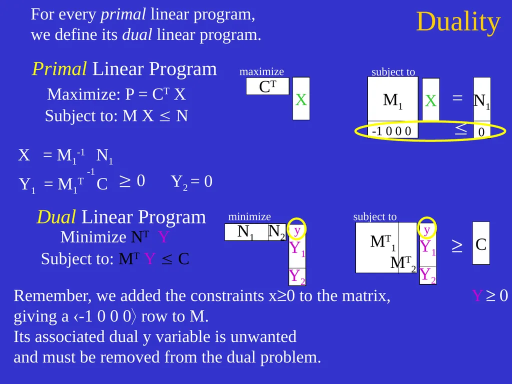
Subject to: MX  N X CT Remember, we added the constraints x³0 to the matrix,
giving a -1 0 0 0 row to M.
Its associated dual y variable is unwantedand must be removed from the dual problem.<br>
slide80. Duality Primal Linear Program For every primal linear program, we define its dual linear program. maximize X Maximize: P = CTX
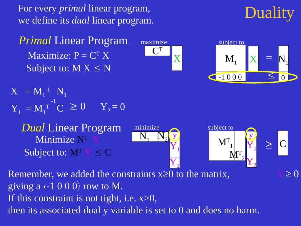
Subject to: MX  N X CT Remember, we added the constraints x³0 to the matrix,
giving a -1 0 0 0 row to M.
If this constraint is not tight, i.e. x>0,
then its associated dual y variable is set to 0 and does no harm.<br>
slide81. Duality Primal Linear Program For every primal linear program, we define its dual linear program. maximize X Maximize: P = CTX
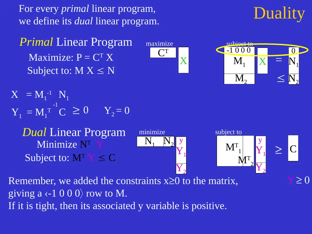
Subject to: MX  N X CT Remember, we added the constraints x³0 to the matrix,giving a -1 0 0 0 row to M.
If it is tight, then its associated y variable is positive. y y<br>
slide82. Duality Primal Linear Program For every primal linear program, we define its dual linear program. maximize X Maximize: P = CTX
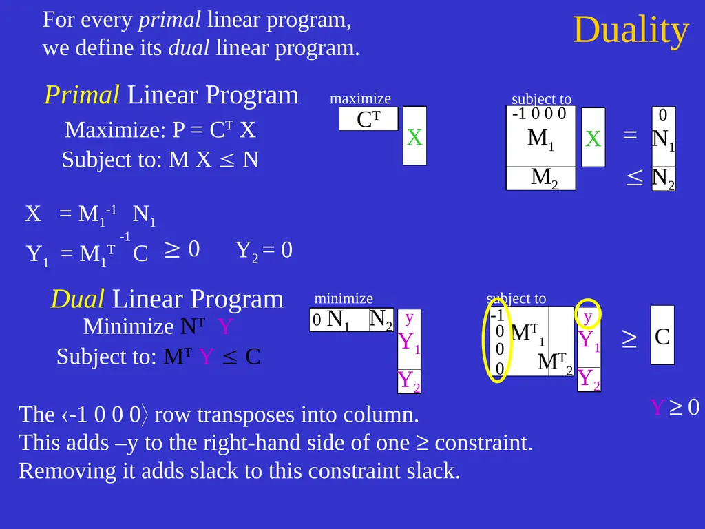
Subject to: MX  N X CT The -1 0 0 0 row transposes into column.
This adds –y to the right-hand side of one ³ constraint.
Removing it adds slack to this constraint slack. y y<br>
slide83. Duality Primal Linear Program For every primal linear program, we define its dual linear program. maximize X Maximize: P = CTX
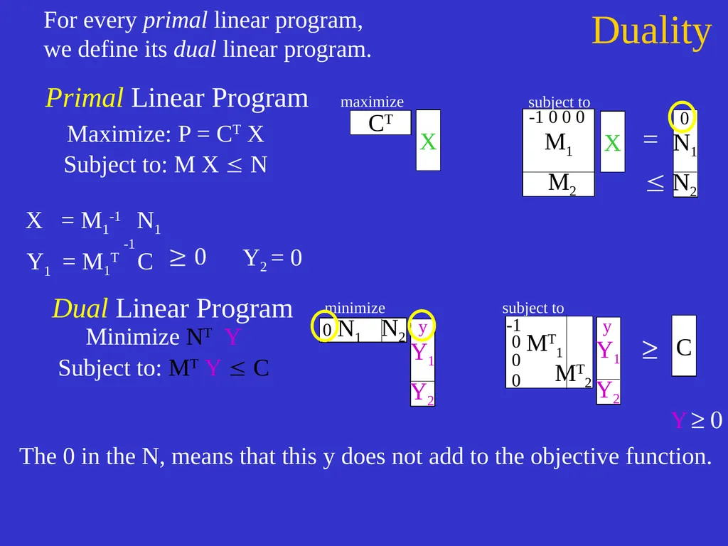
Subject to: MX  N X CT The 0 in the N, means that this y does not add to the objective function. y y<br>
slide84. Duality Primal Linear Program For every primal linear program, we define its dual linear program. maximize X Maximize: P = CTX
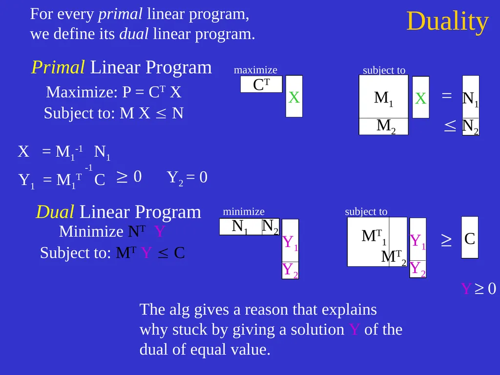
Subject to: MX  N X CT The alg gives a reason that explains why stuck by giving a solution Y of the dual of equal value.<br>
slide85. Duality Primal Linear Program For every primal linear program, we define its dual linear program. maximize X Maximize: P = CTX
Subject to: MX  N X CT<br>
slide86. End<br>
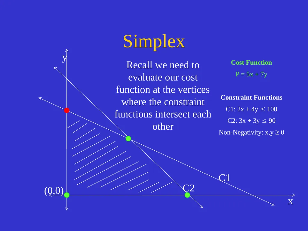
slide87. Simplex C1 C2 (0,0) y x Cost Function
P = 5x + 7y

Constraint Functions
C1: 2x + 4y  100
C2: 3x + 3y  90
Non-Negativity: x,y ³ 0 Recall we need to evaluate our cost function at the vertices where the constraint functions intersect each other<br>
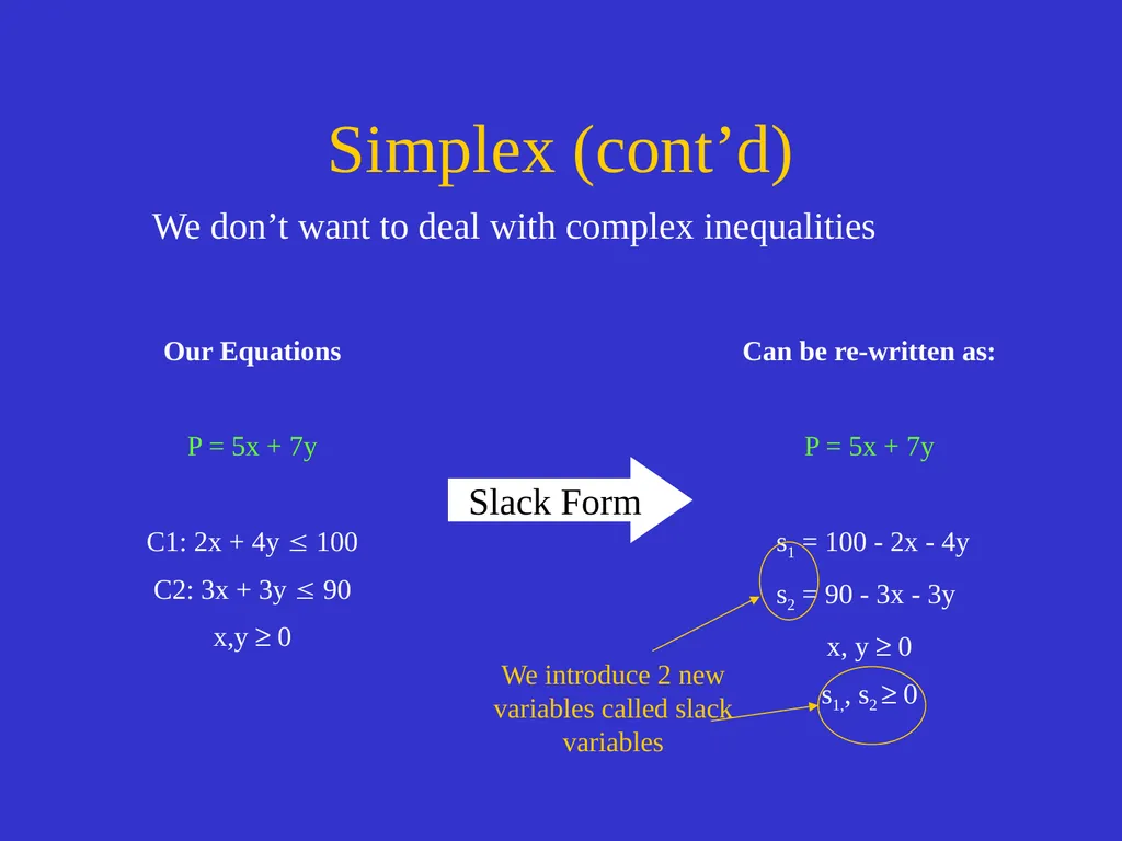
slide88. Simplex (cont’d) Our Equations

P = 5x + 7y

C1: 2x + 4y  100
C2: 3x + 3y  90
x,y ³ 0 Slack Form Can be re-written as:

P = 5x + 7y

s1 = 100 - 2x - 4y
s2 = 90 - 3x - 3y
x, y ³ 0
s1,, s2 ³ 0 We don’t want to deal with complex inequalities<br>
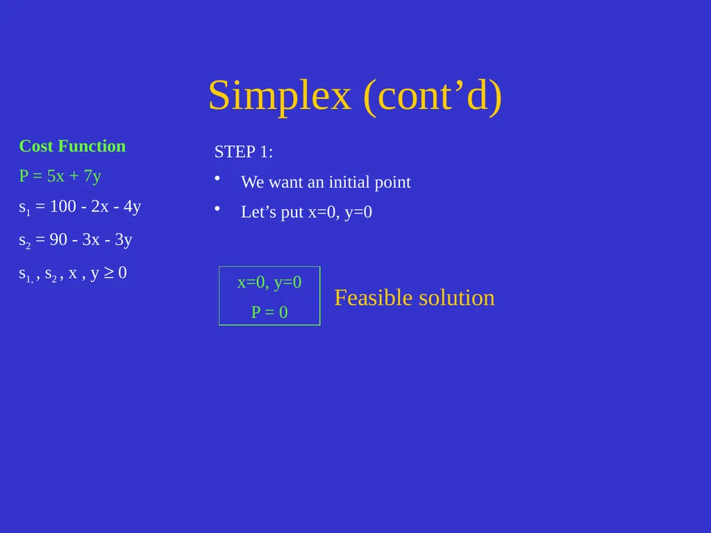
slide89. Simplex (cont’d) Cost Function
P = 5x + 7y
s1 = 100 - 2x - 4y
s2 = 90 - 3x - 3y
s1, , s2 , x , y ³ 0 STEP 1:
We want an initial point
Let’s put x=0, y=0 Feasible solution x=0, y=0
P = 0<br>
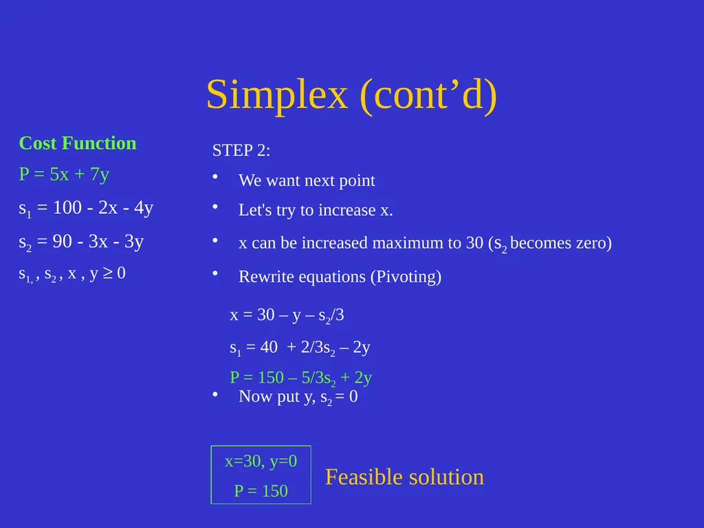
slide90. Simplex (cont’d) Cost Function
P = 5x + 7y
s1 = 100 - 2x - 4y
s2 = 90 - 3x - 3y
s1, , s2 , x , y ³ 0 STEP 2:
We want next point
Let's try to increase x.
x can be increased maximum to 30 (s2 becomes zero)
Rewrite equations (Pivoting)

Now put y, s2 = 0 Feasible solution x = 30 – y – s2/3
s1 = 40 + 2/3s2 – 2y
P = 150 – 5/3s2 + 2y x=30, y=0
P = 150<br>
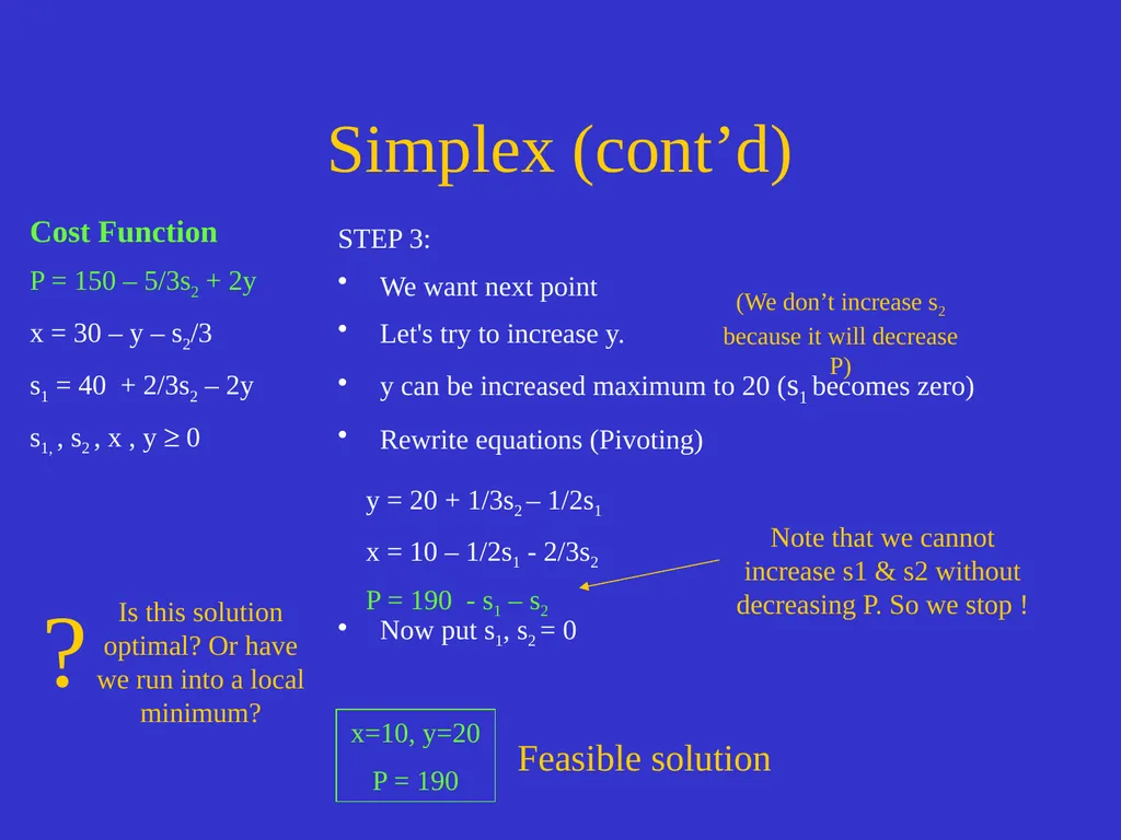
slide91. Simplex (cont’d) Cost Function
P = 150 – 5/3s2 + 2y
x = 30 – y – s2/3
s1 = 40 + 2/3s2 – 2y
s1, , s2 , x , y ³ 0 STEP 3:
We want next point
Let's try to increase y.
y can be increased maximum to 20 (s1 becomes zero)
Rewrite equations (Pivoting)

Now put s1, s2 = 0 y = 20 + 1/3s2 – 1/2s1
x = 10 – 1/2s1 - 2/3s2
P = 190 - s1 – s2 x=10, y=20
P = 190 (We don’t increase s2 because it will decrease P) Feasible solution<br>