
Linear Systems – Iterative methods Jacobi Method
Description: Linear Systems Iterative methods Jacobi Method Gauss-Siedel Method 1 Iterative Methods Iterative methods can be expressed in the general form: x(k) F(x(k-1)) where s s.t. F(s)s is called a Fixed Point Hopefully: x(k) s (solution of my
Related Topics
Download Presentation
"Linear Systems – Iterative methods Jacobi Method" is the property of its rightful owner. Permission is granted to download and print the materials on this website for personal, non-commercial use only, and to display it on your personal computer provided you do not modify the materials and that you retain all copyright notices contained in the materials. By downloading content from our website, you accept the terms of this agreement.
Presentation Transcript
slide1. Linear Systems – Iterative methods Jacobi Method
Gauss-Siedel Method 1<br>
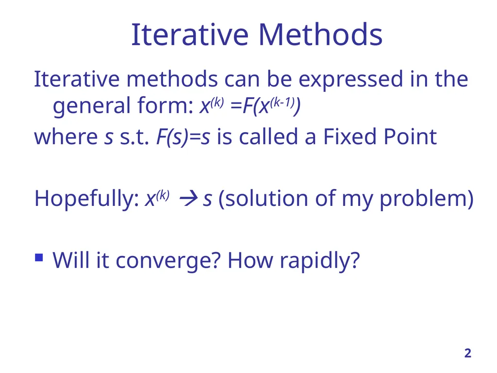
slide2. Iterative Methods Iterative methods can be expressed in the general form: x(k) =F(x(k-1))
where s s.t. F(s)=s is called a Fixed Point
Hopefully: x(k) s (solution of my problem)
Will it converge? How rapidly? 2<br>
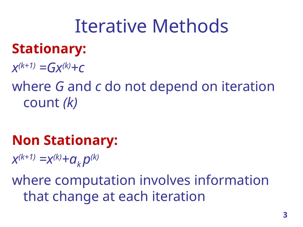
slide3. Iterative Methods Stationary:
x(k+1) =Gx(k)+c
where G and c do not depend on iteration count (k)
Non Stationary:
x(k+1) =x(k)+ak p(k)
where computation involves information that change at each iteration 3<br>
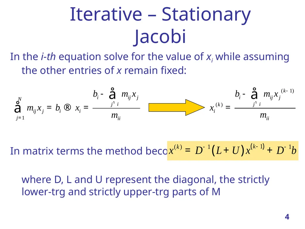
slide4. Iterative – Stationary Jacobi In the i-th equation solve for the value of xi while assuming the other entries of x remain fixed:
In matrix terms the method becomes:
where D, L and U represent the diagonal, the strictly lower-trg and strictly upper-trg parts of M 4<br>
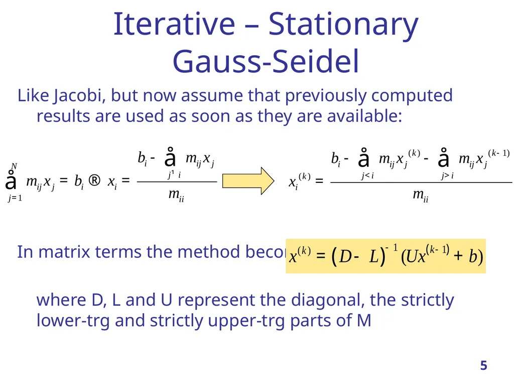
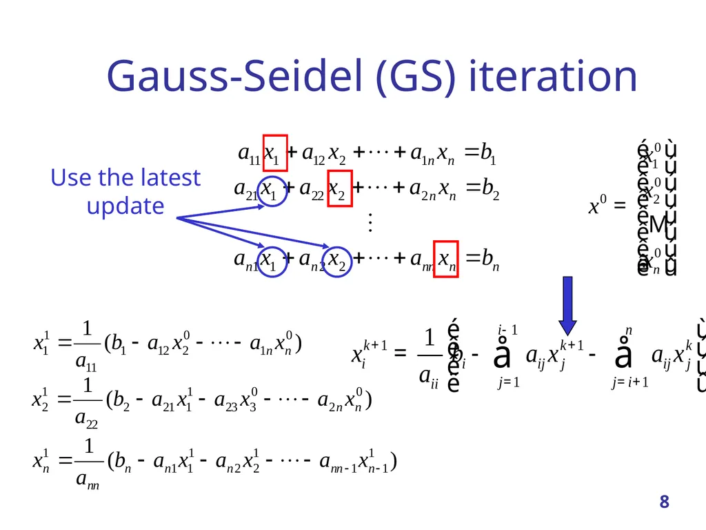
slide5. Iterative – Stationary Gauss-Seidel Like Jacobi, but now assume that previously computed results are used as soon as they are available:
In matrix terms the method becomes:
where D, L and U represent the diagonal, the strictly lower-trg and strictly upper-trg parts of M 5<br>
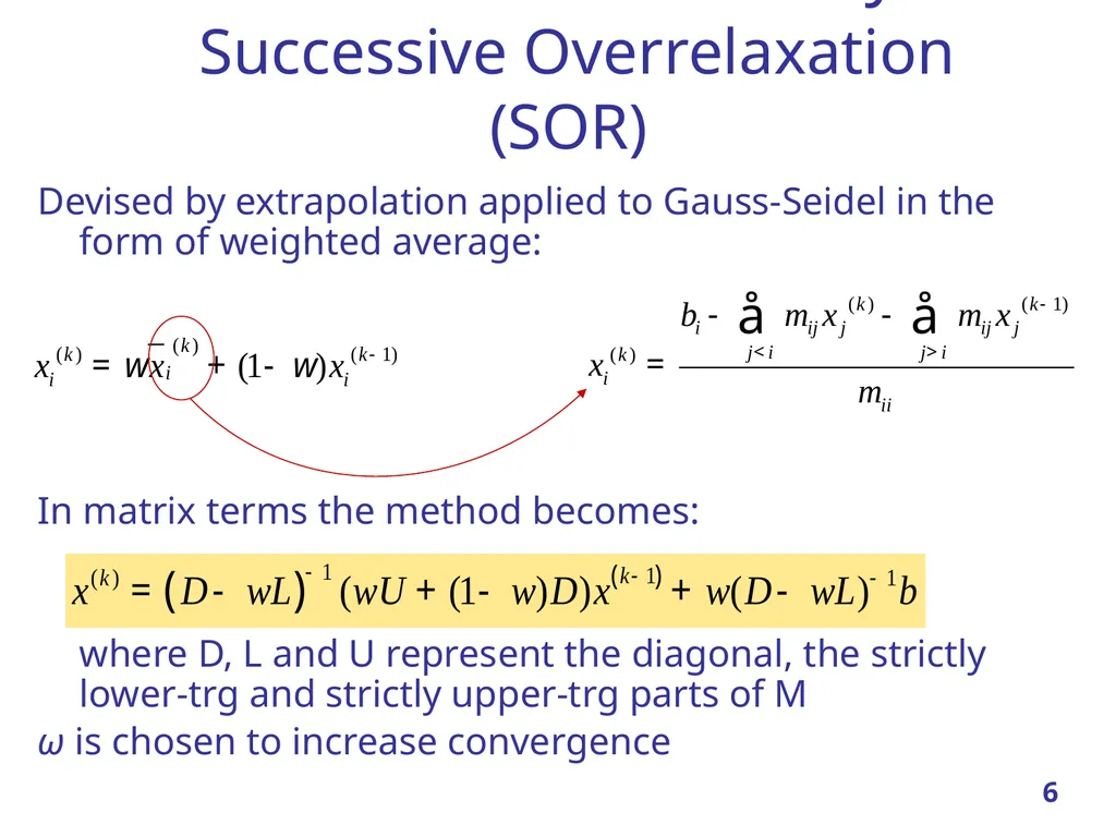
slide6. Iterative – Stationary Successive Overrelaxation (SOR) Devised by extrapolation applied to Gauss-Seidel in the form of weighted average:
In matrix terms the method becomes:
where D, L and U represent the diagonal, the strictly lower-trg and strictly upper-trg parts of M
ω is chosen to increase convergence 6<br>
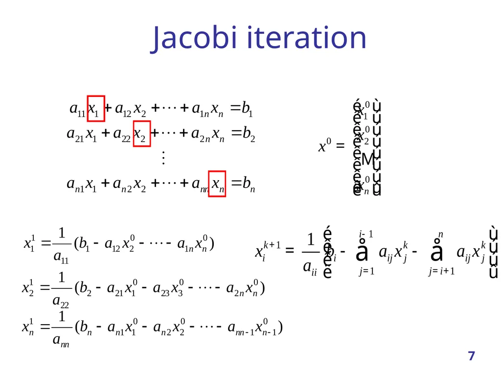
slide7. 7 Jacobi iteration<br>
slide8. 8 Gauss-Seidel (GS) iteration<br>
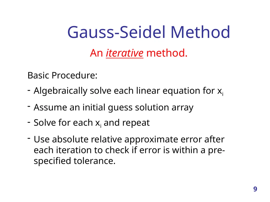
slide9. Gauss-Seidel Method An iterative method. Basic Procedure:
Algebraically solve each linear equation for xi
Assume an initial guess solution array
Solve for each xi and repeat
Use absolute relative approximate error after each iteration to check if error is within a pre-specified tolerance. 9<br>
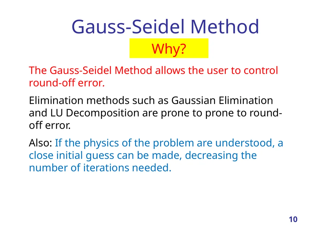
slide10. Gauss-Seidel Method Why? The Gauss-Seidel Method allows the user to control round-off error.
Elimination methods such as Gaussian Elimination and LU Decomposition are prone to prone to round-off error.
Also: If the physics of the problem are understood, a close initial guess can be made, decreasing the number of iterations needed. 10<br>
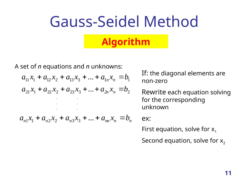
slide11. Gauss-Seidel Method Algorithm A set of n equations and n unknowns: . .
. .
. . If: the diagonal elements are non-zero
Rewrite each equation solving for the corresponding unknown
ex:
First equation, solve for x1
Second equation, solve for x2 11<br>
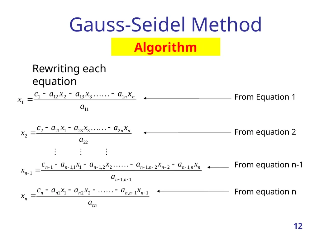
slide12. Gauss-Seidel Method Algorithm Rewriting each equation From Equation 1
From equation 2
From equation n-1
From equation n 12<br>
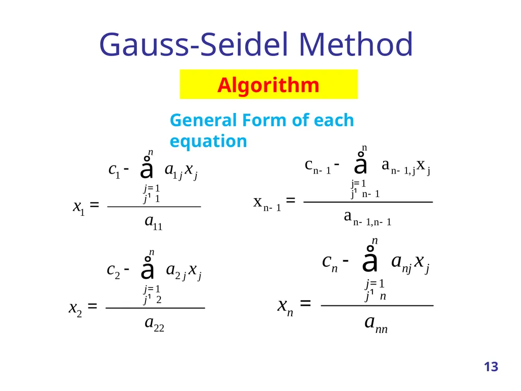
slide13. Gauss-Seidel Method Algorithm General Form of each equation 13<br>
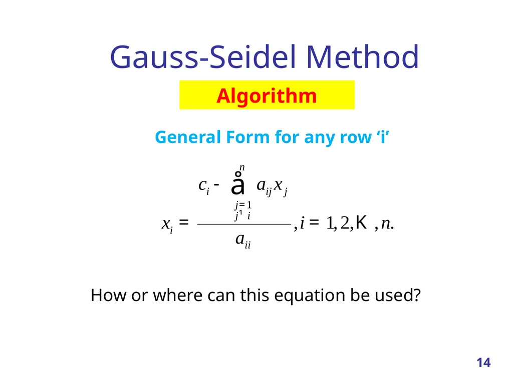
slide14. Gauss-Seidel Method Algorithm General Form for any row ‘i’ How or where can this equation be used? 14<br>
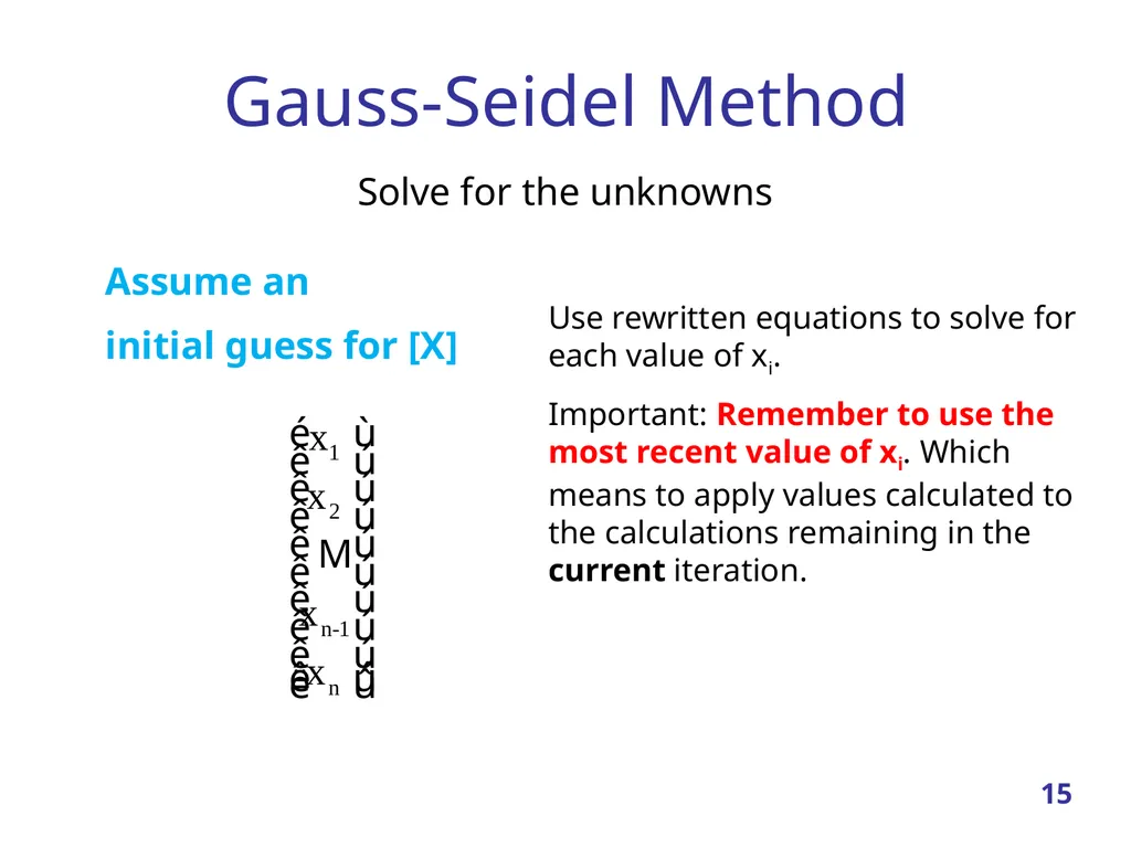
slide15. Gauss-Seidel Method Solve for the unknowns Assume an
initial guess for [X] Use rewritten equations to solve for each value of xi.
Important: Remember to use the most recent value of xi. Which means to apply values calculated to the calculations remaining in the current iteration. 15<br>
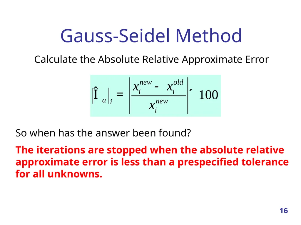
slide16. Gauss-Seidel Method Calculate the Absolute Relative Approximate Error So when has the answer been found?
The iterations are stopped when the absolute relative approximate error is less than a prespecified tolerance for all unknowns. 16<br>
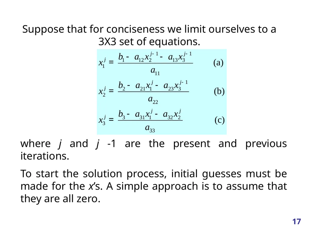
slide17. 17 Suppose that for conciseness we limit ourselves to a 3X3 set of equations. where j and j -1 are the present and previous iterations.
To start the solution process, initial guesses must be made for the x’s. A simple approach is to assume that they are all zero.<br>
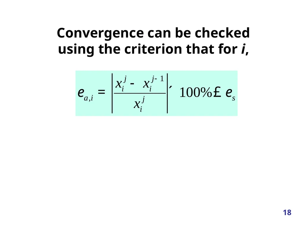
slide18. 18 Convergence can be checked using the criterion that for i,<br>
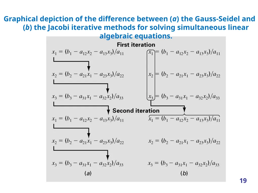
slide19. 19 Graphical depiction of the difference between (a) the Gauss-Seidel and (b) the Jacobi iterative methods for solving simultaneous linear algebraic equations.<br>
slide20. Jacobi's Method 20 https://www.maa.org/press/periodicals/loci/joma/iterative-methods-for-solving-iaxi-ibi-jacobis-method Perhaps the simplest iterative method for solving Ax=b is Jacobi’s Method.
Note that the simplicity of this method is both good and bad:
good, because it is relatively easy to understand and thus is a good first taste of iterative methods;
bad, because it is not typically used in practice (although its potential usefulness has been reconsidered with the advent of parallel computing).
Still, it is a good starting point for learning about more useful, but more complicated, iterative methods.<br>
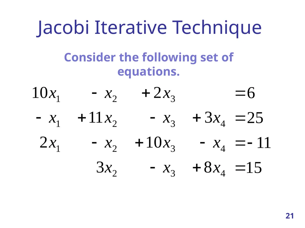
slide21. Jacobi Iterative Technique Consider the following set of equations. 21<br>
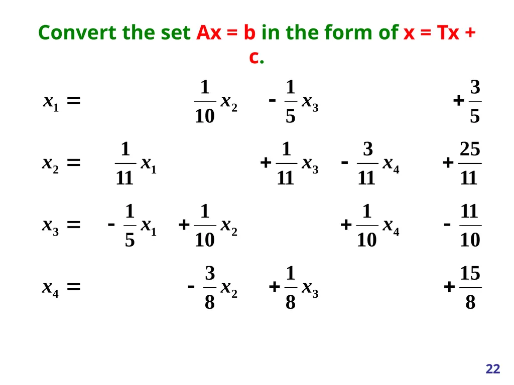
slide22. Convert the set Ax = b in the form of x = Tx + c. 22<br>
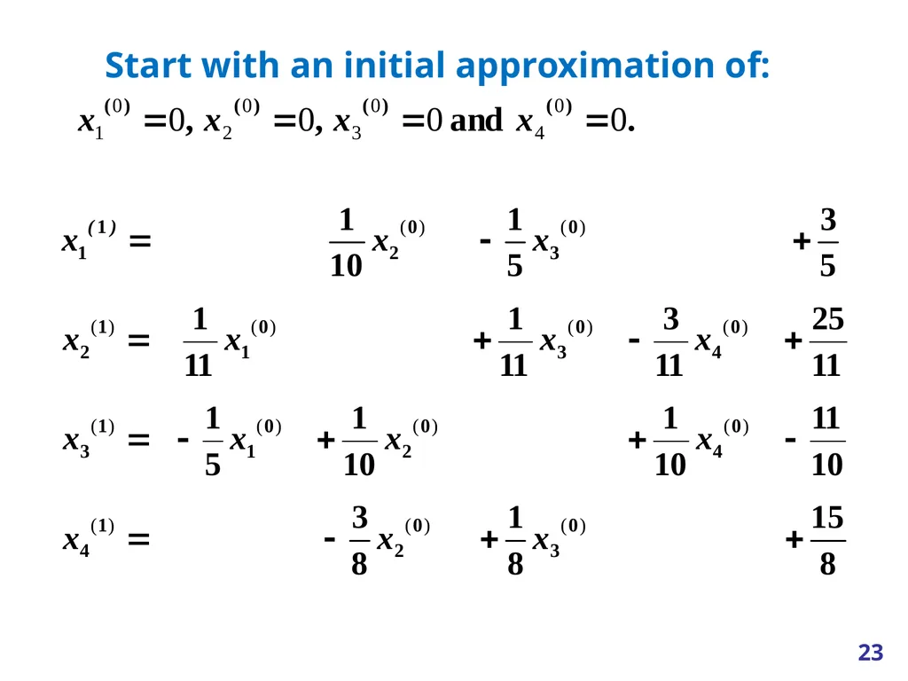
slide23. Start with an initial approximation of: 23<br>
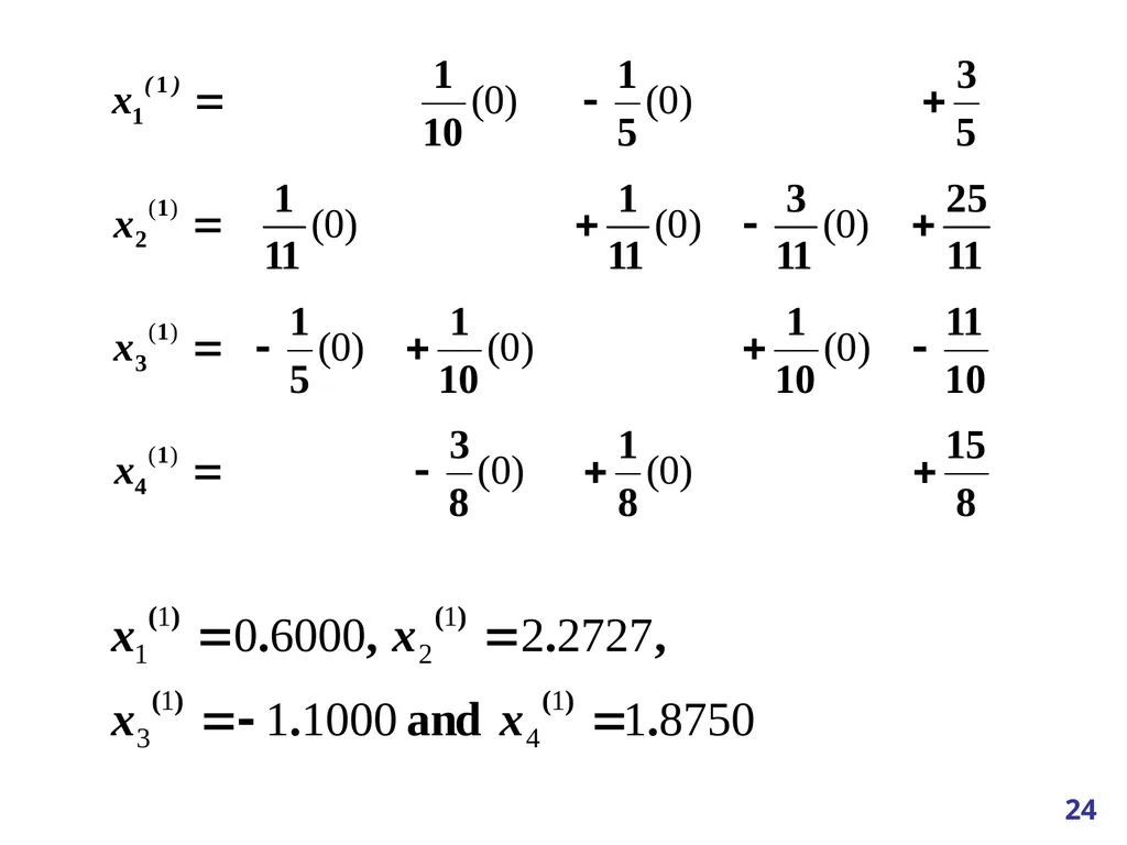
slide24. 24<br>
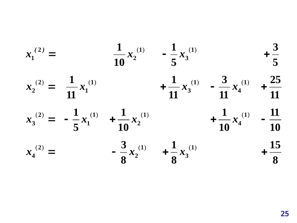
slide25. 25<br>
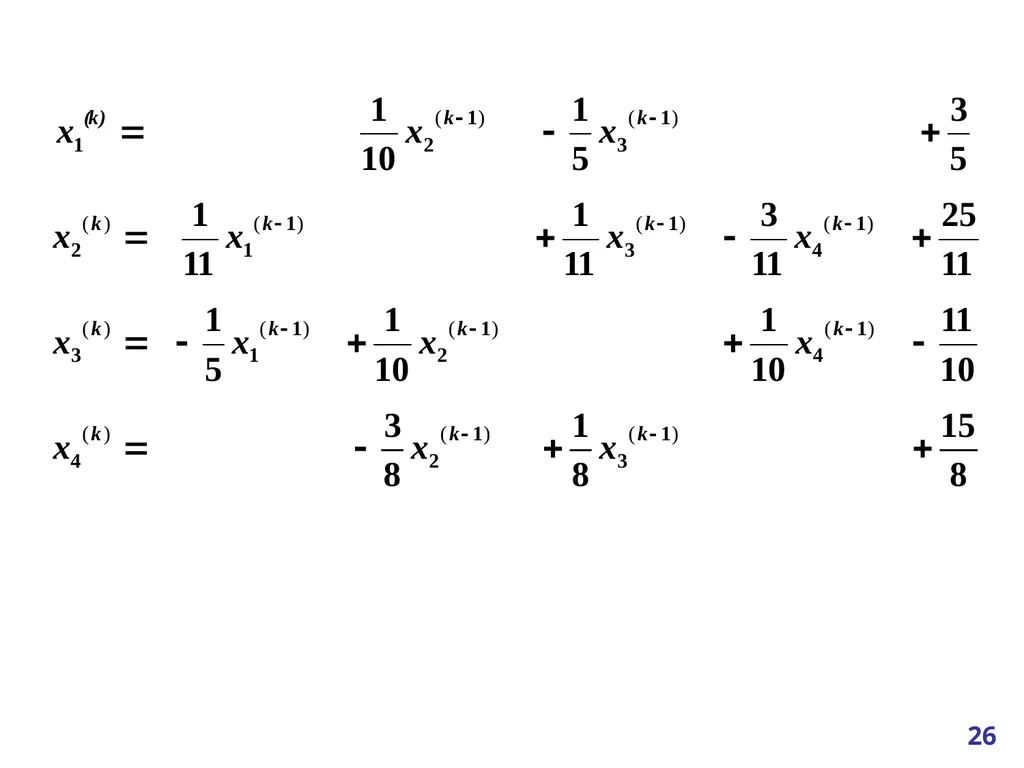
slide26. 26<br>
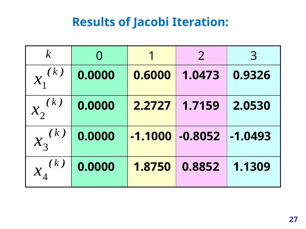
slide27. Results of Jacobi Iteration: 27<br>
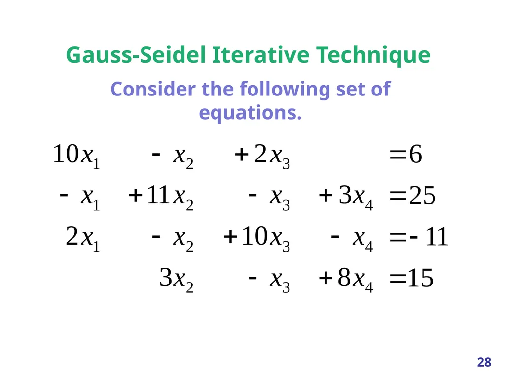
slide28. Gauss-Seidel Iterative Technique Consider the following set of equations. 28<br>
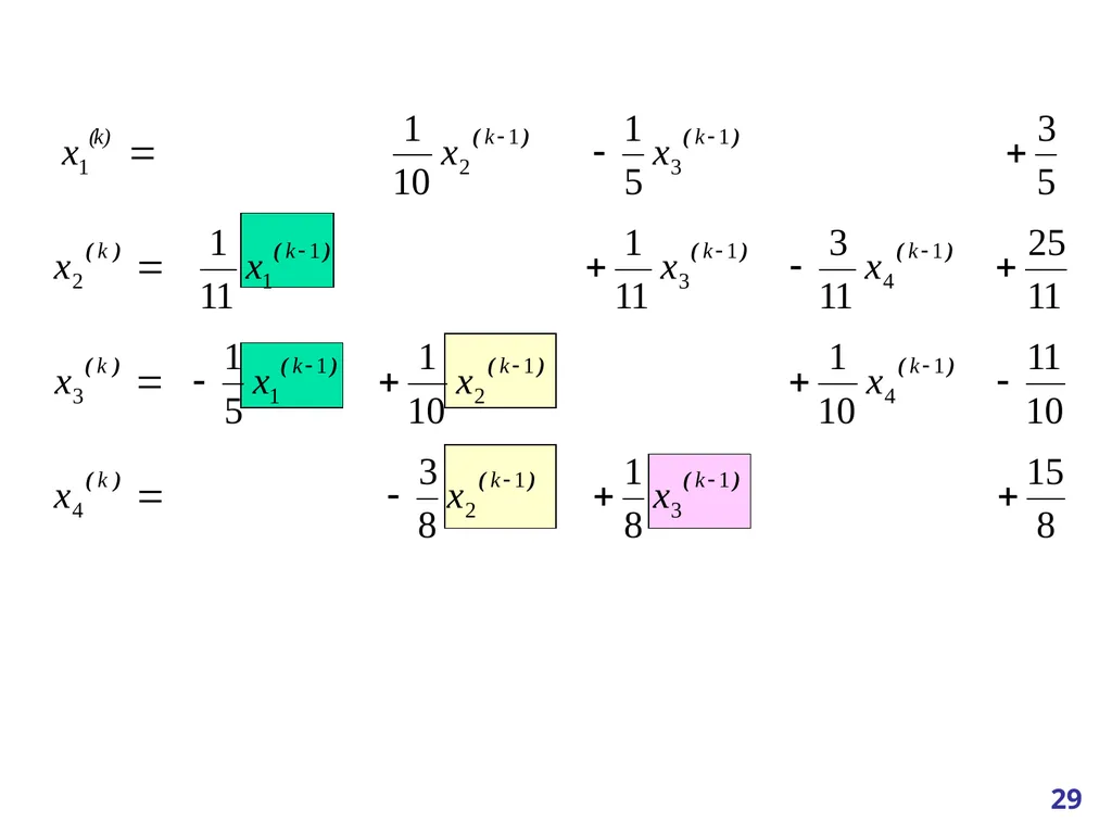
slide29. 29<br>
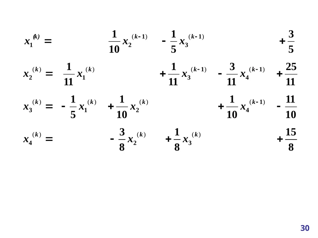
slide30. 30<br>
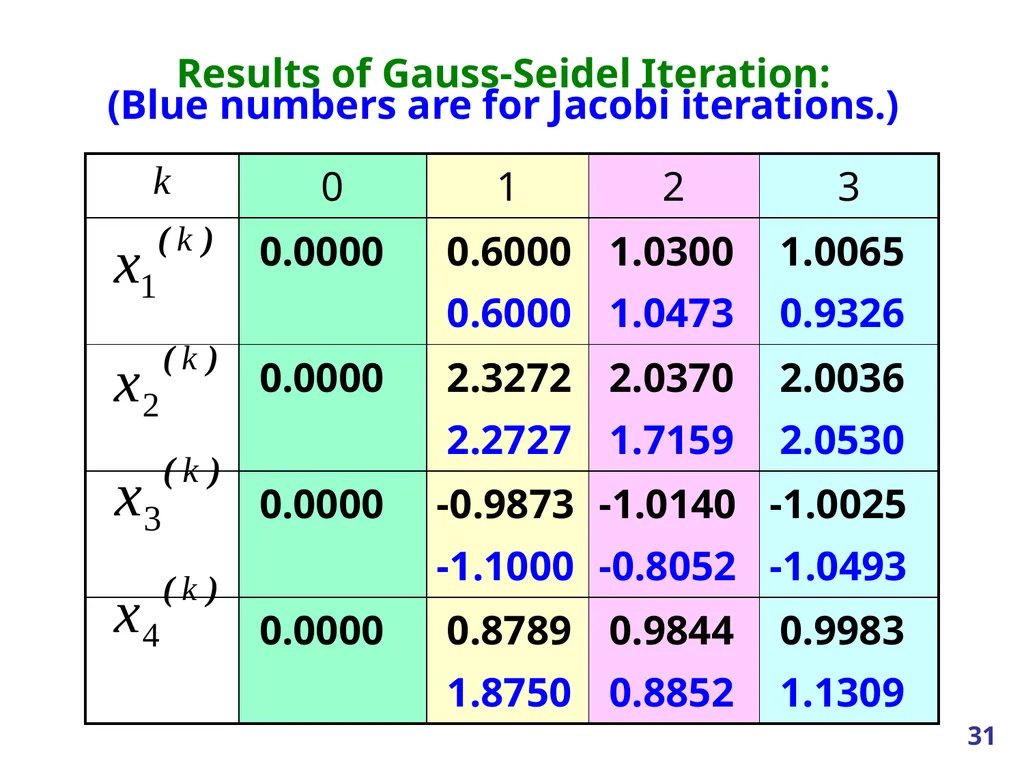
slide31. Results of Gauss-Seidel Iteration:
(Blue numbers are for Jacobi iterations.) 31<br>
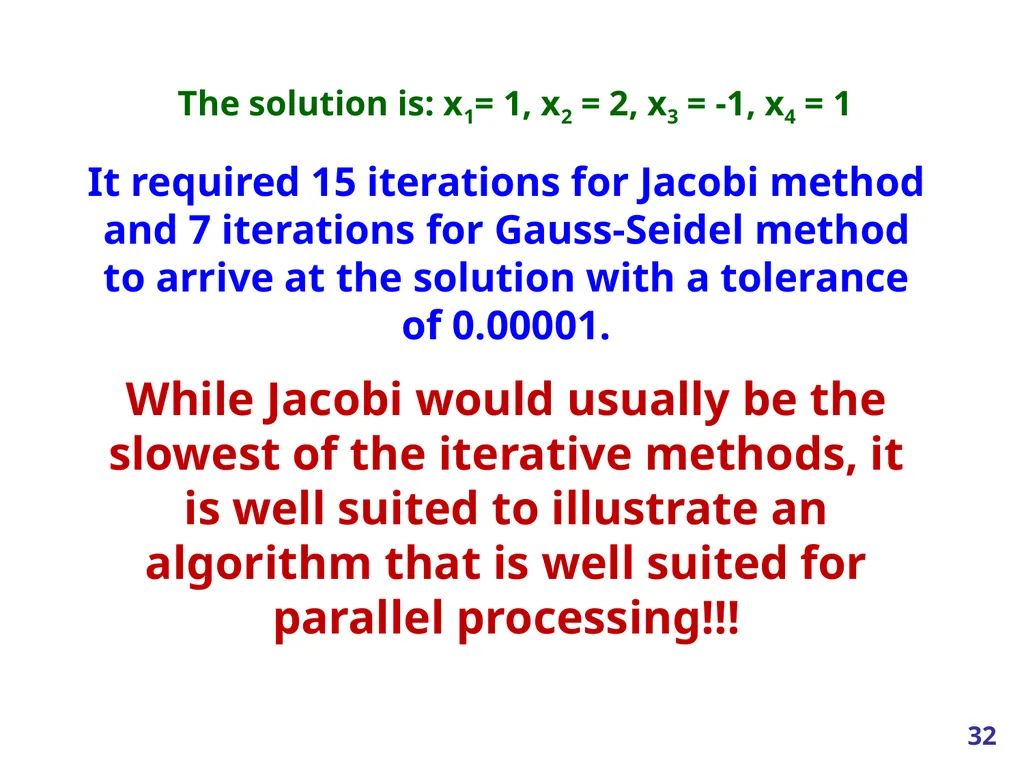
slide32. It required 15 iterations for Jacobi method and 7 iterations for Gauss-Seidel method to arrive at the solution with a tolerance of 0.00001.
While Jacobi would usually be the slowest of the iterative methods, it is well suited to illustrate an algorithm that is well suited for parallel processing!!! The solution is: x1= 1, x2 = 2, x3 = -1, x4 = 1 32<br>
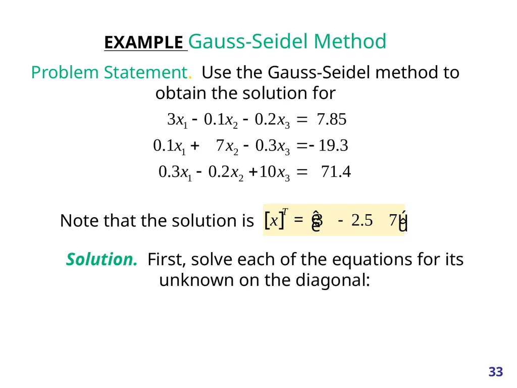
slide33. 33 EXAMPLE Gauss-Seidel Method
Problem Statement. Use the Gauss-Seidel method to obtain the solution for Note that the solution is Solution. First, solve each of the equations for its unknown on the diagonal:<br>
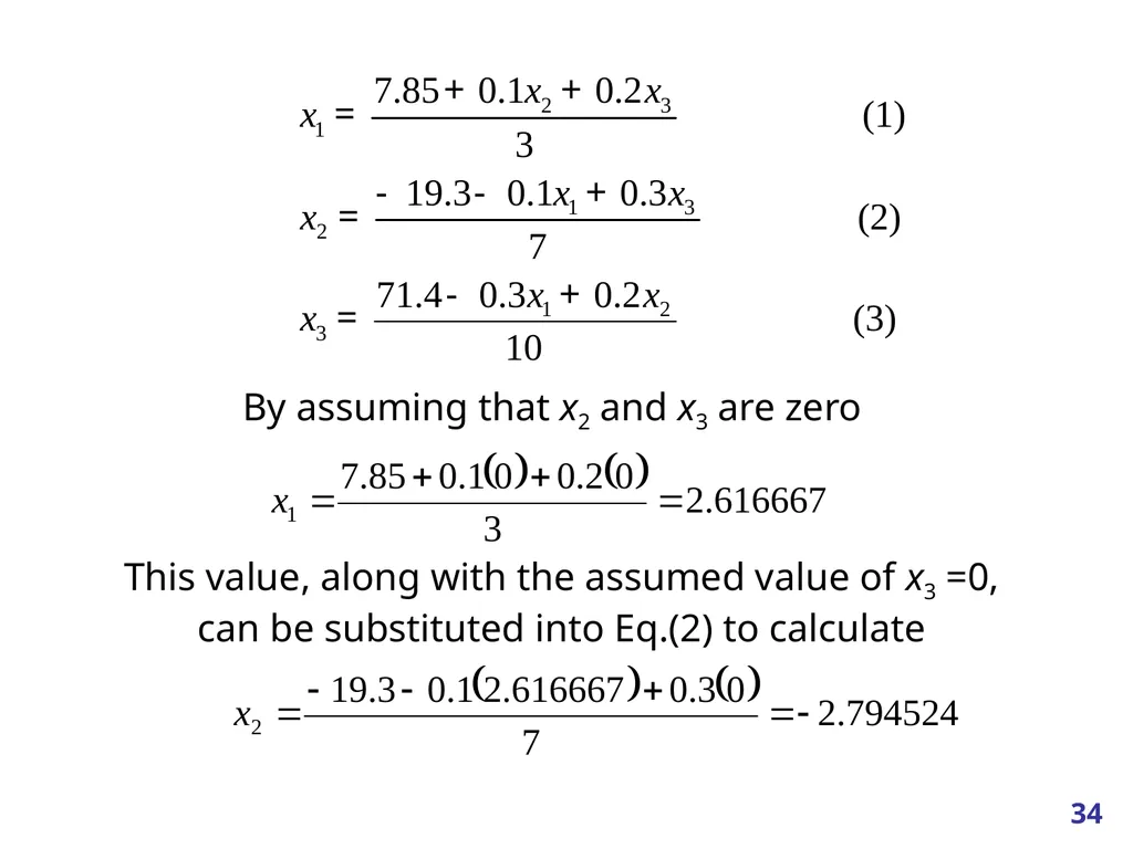
slide34. 34 By assuming that x2 and x3 are zero This value, along with the assumed value of x3 =0, can be substituted into Eq.(2) to calculate<br>
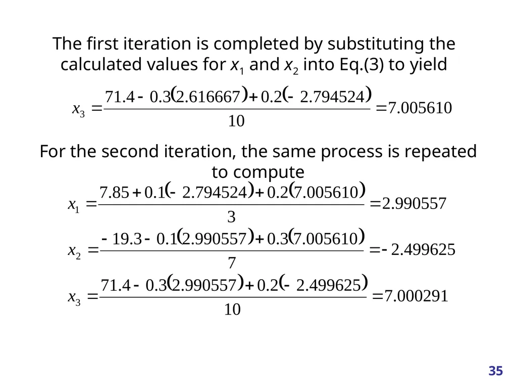
slide35. 35 The first iteration is completed by substituting the calculated values for x1 and x2 into Eq.(3) to yield For the second iteration, the same process is repeated to compute<br>
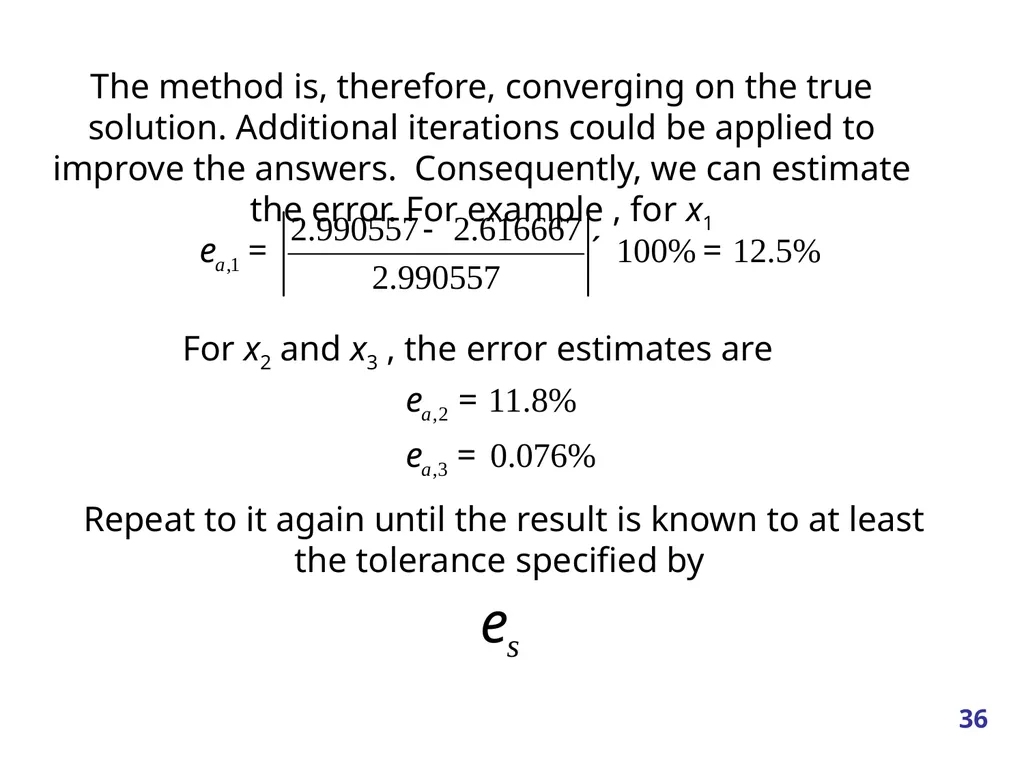
slide36. 36 The method is, therefore, converging on the true solution. Additional iterations could be applied to improve the answers. Consequently, we can estimate the error. For example , for x1 For x2 and x3 , the error estimates are Repeat to it again until the result is known to at least the tolerance specified by<br>
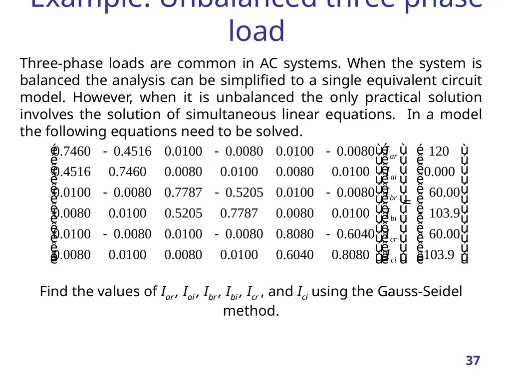
slide37. Example: Unbalanced three phase load Three-phase loads are common in AC systems. When the system is balanced the analysis can be simplified to a single equivalent circuit model. However, when it is unbalanced the only practical solution involves the solution of simultaneous linear equations. In a model the following equations need to be solved. Find the values of Iar , Iai , Ibr , Ibi , Icr , and Ici using the Gauss-Seidel method. 37<br>
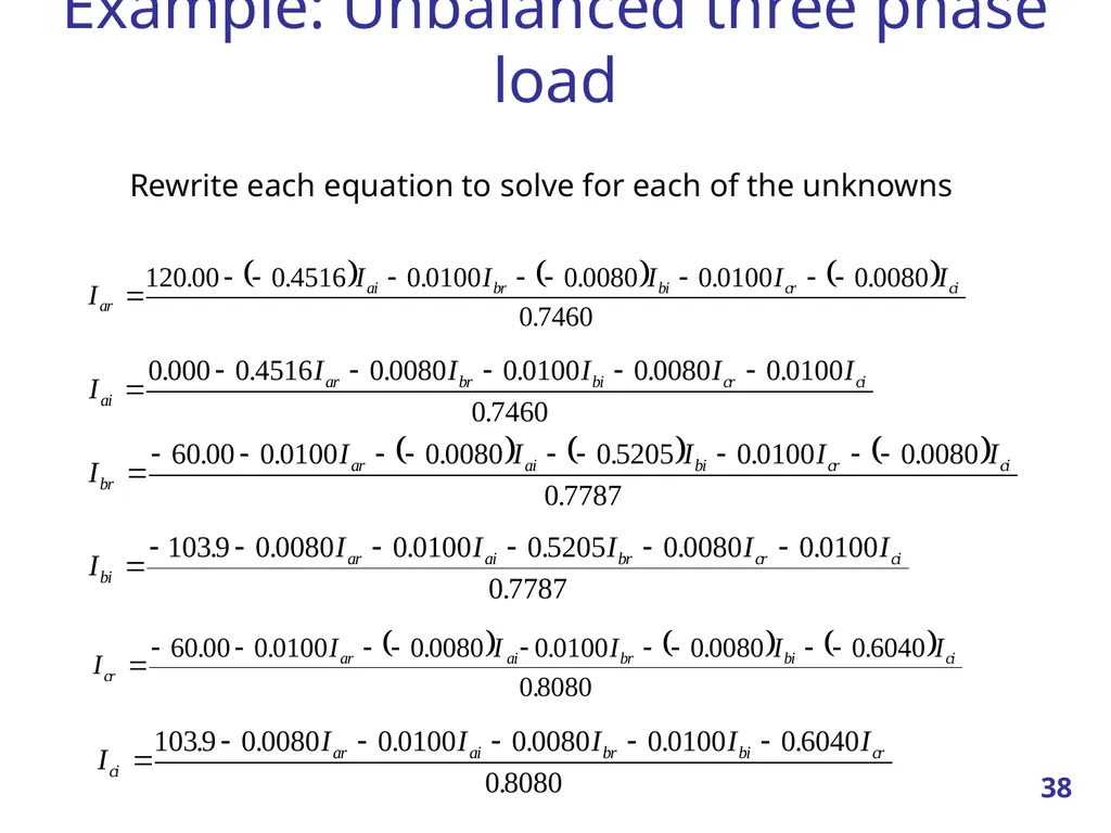
slide38. Example: Unbalanced three phase load Rewrite each equation to solve for each of the unknowns 38<br>
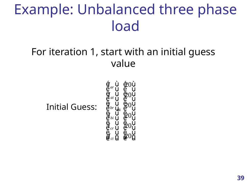
slide39. Example: Unbalanced three phase load Initial Guess: For iteration 1, start with an initial guess value 39<br>
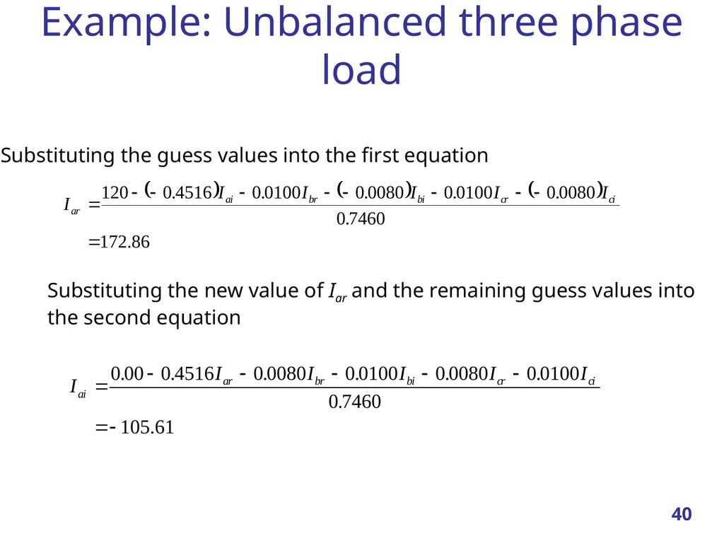
slide40. Example: Unbalanced three phase load Substituting the guess values into the first equation Substituting the new value of Iar and the remaining guess values into
the second equation 40<br>
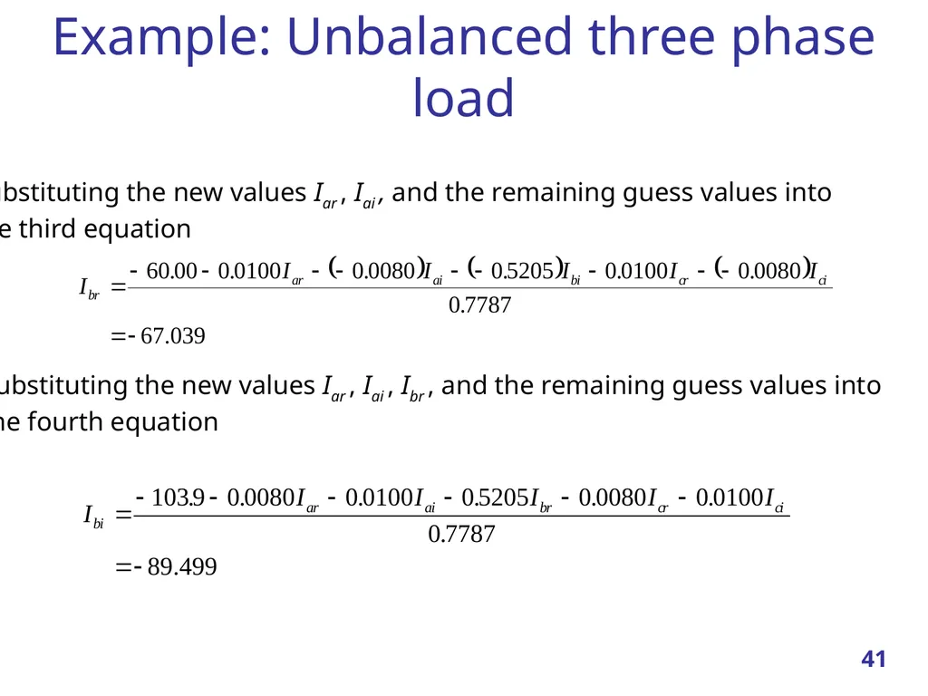
slide41. Example: Unbalanced three phase load Substituting the new values Iar , Iai , and the remaining guess values into
the third equation Substituting the new values Iar , Iai , Ibr , and the remaining guess values into
the fourth equation 41<br>
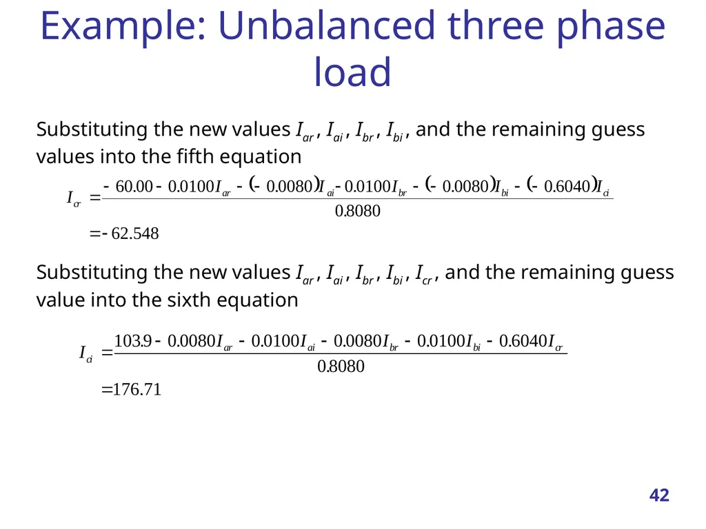
slide42. Example: Unbalanced three phase load Substituting the new values Iar , Iai , Ibr , Ibi , and the remaining guess values into the fifth equation Substituting the new values Iar , Iai , Ibr , Ibi , Icr , and the remaining guess value into the sixth equation 42<br>
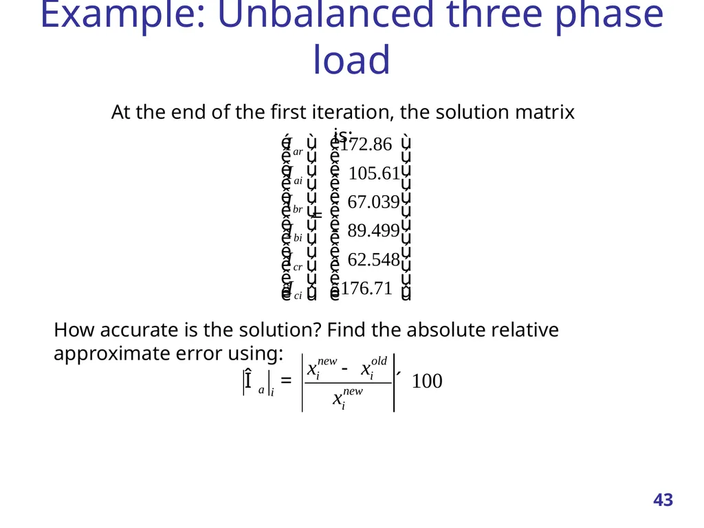
slide43. Example: Unbalanced three phase load How accurate is the solution? Find the absolute relative approximate error using: At the end of the first iteration, the solution matrix is: 43<br>
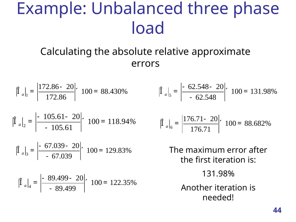
slide44. Example: Unbalanced three phase load Calculating the absolute relative approximate errors The maximum error after the first iteration is:
131.98%
Another iteration is needed! 44<br>
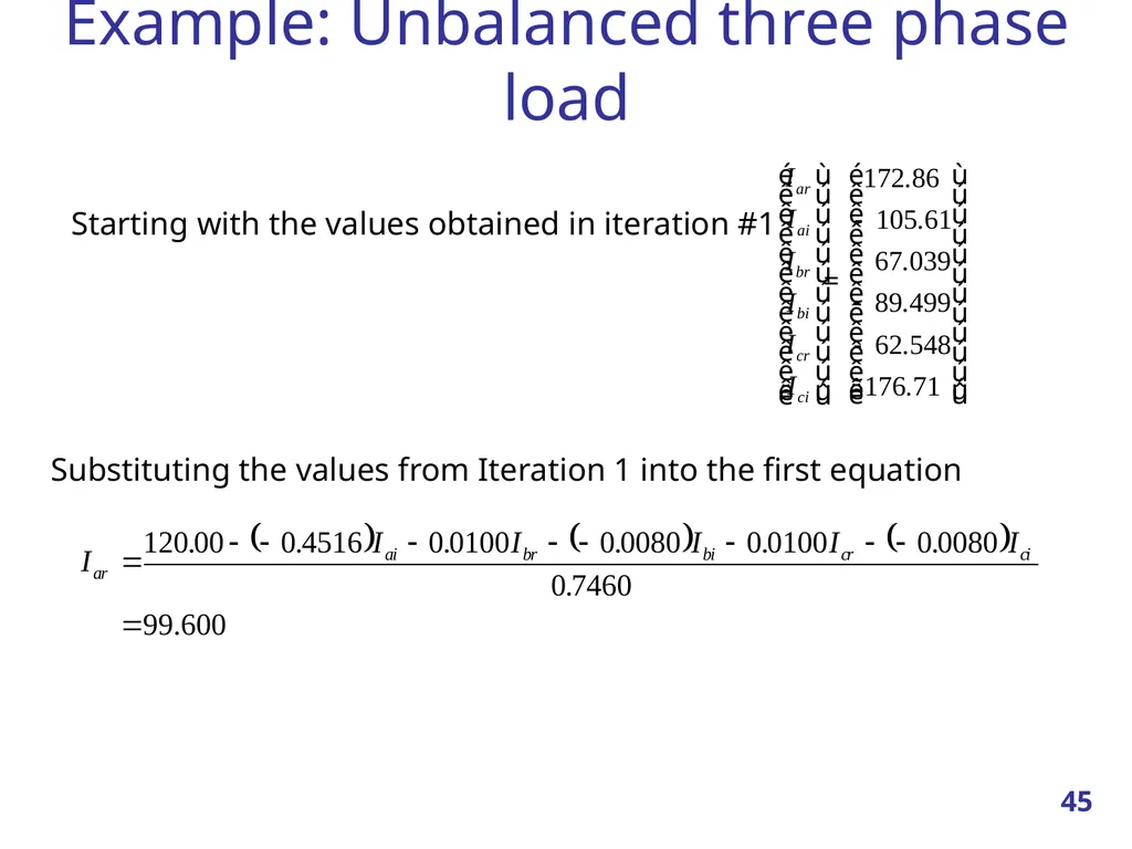
slide45. Example: Unbalanced three phase load Starting with the values obtained in iteration #1 Substituting the values from Iteration 1 into the first equation 45<br>
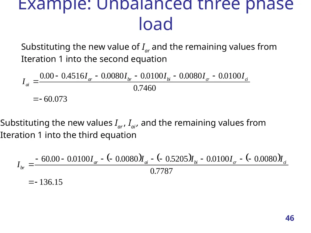
slide46. Example: Unbalanced three phase load Substituting the new value of Iar and the remaining values from
Iteration 1 into the second equation Substituting the new values Iar , Iai , and the remaining values from
Iteration 1 into the third equation 46<br>
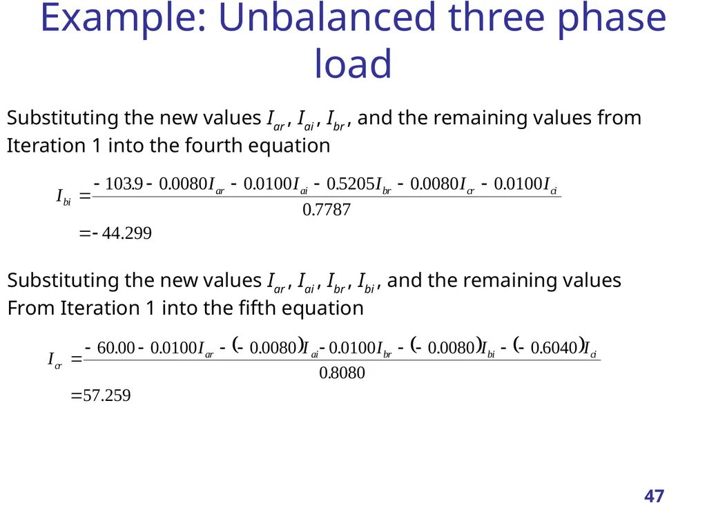
slide47. Example: Unbalanced three phase load Substituting the new values Iar , Iai , Ibr , and the remaining values from
Iteration 1 into the fourth equation Substituting the new values Iar , Iai , Ibr , Ibi , and the remaining values
From Iteration 1 into the fifth equation 47<br>
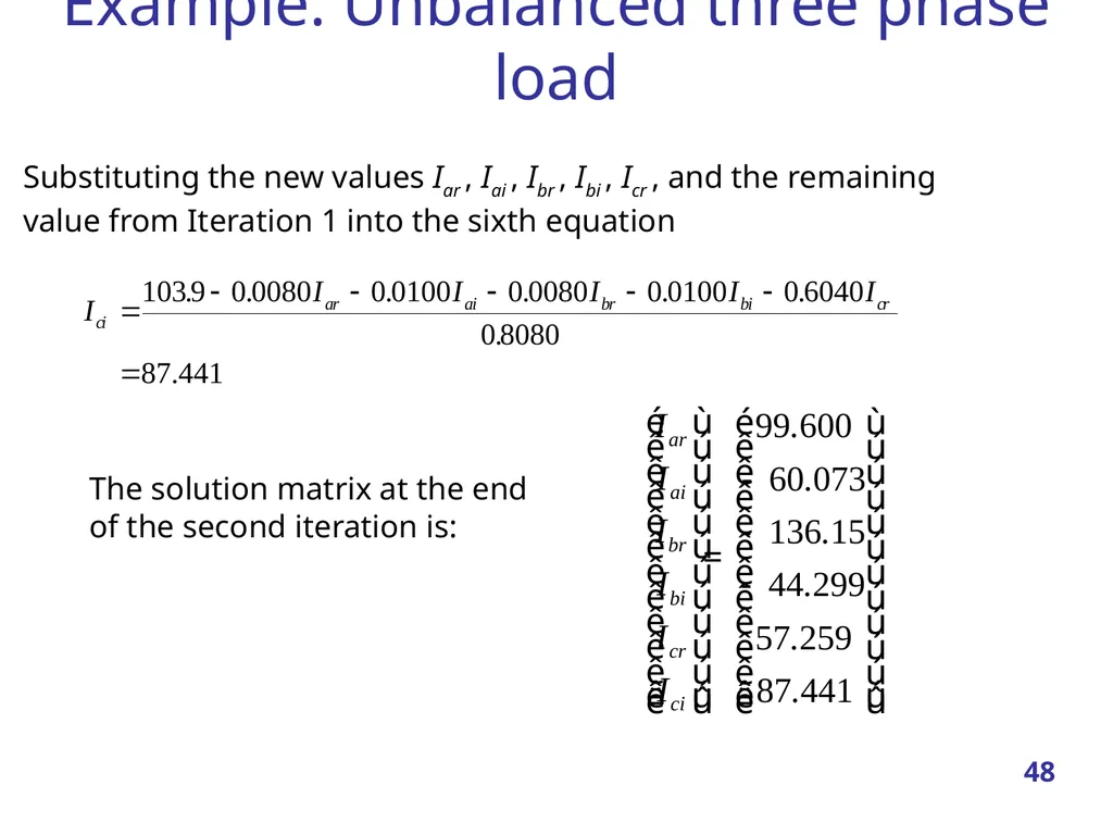
slide48. Example: Unbalanced three phase load Substituting the new values Iar , Iai , Ibr , Ibi , Icr , and the remaining
value from Iteration 1 into the sixth equation The solution matrix at the end of the second iteration is: 48<br>
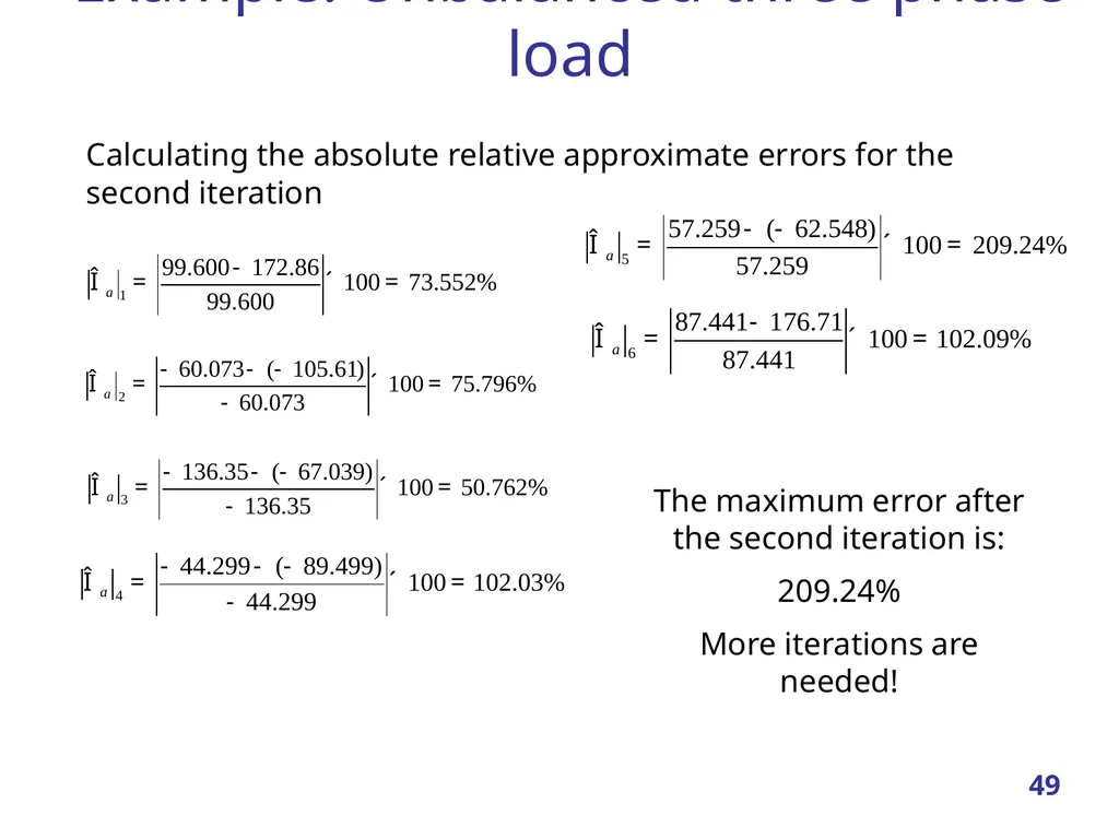
slide49. Example: Unbalanced three phase load Calculating the absolute relative approximate errors for the second iteration The maximum error after the second iteration is:
209.24%
More iterations are needed! 49<br>
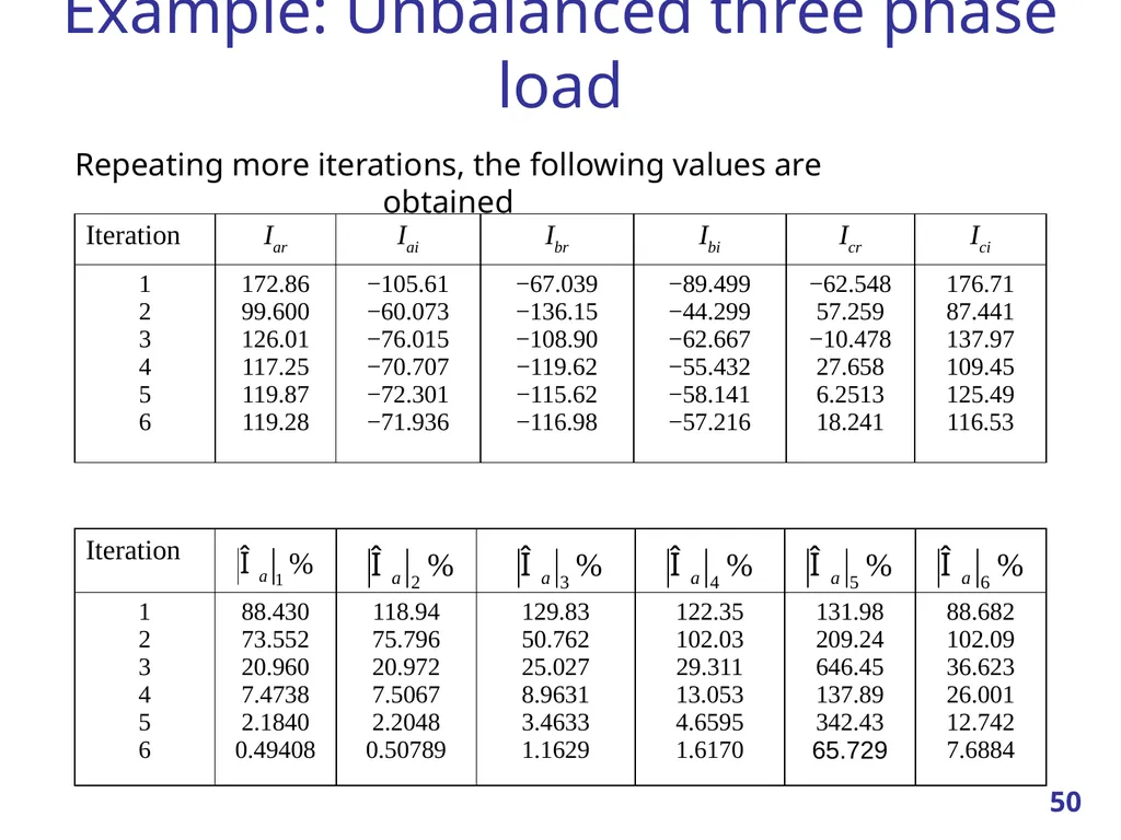
slide50. Example: Unbalanced three phase load Repeating more iterations, the following values are obtained 50<br>
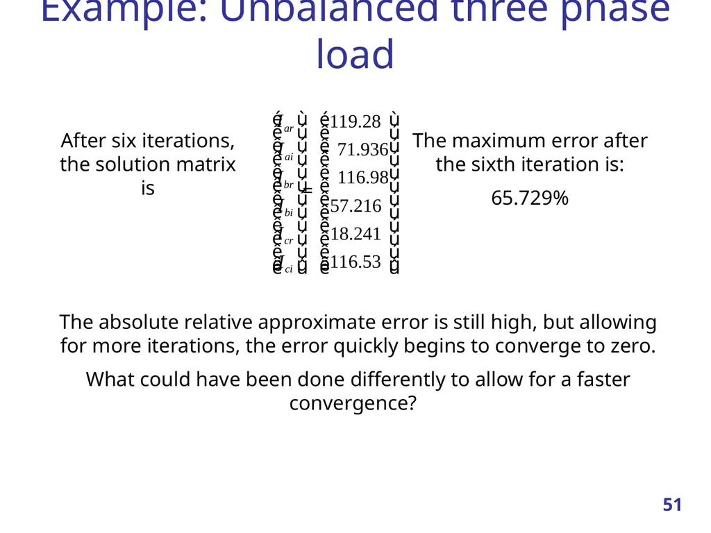
slide51. Example: Unbalanced three phase load The absolute relative approximate error is still high, but allowing for more iterations, the error quickly begins to converge to zero.
What could have been done differently to allow for a faster convergence? After six iterations, the solution matrix is The maximum error after the sixth iteration is:
65.729% 51<br>
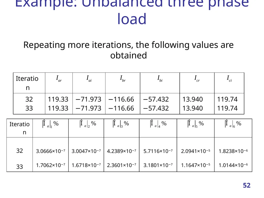
slide52. Example: Unbalanced three phase load Repeating more iterations, the following values are obtained 52<br>
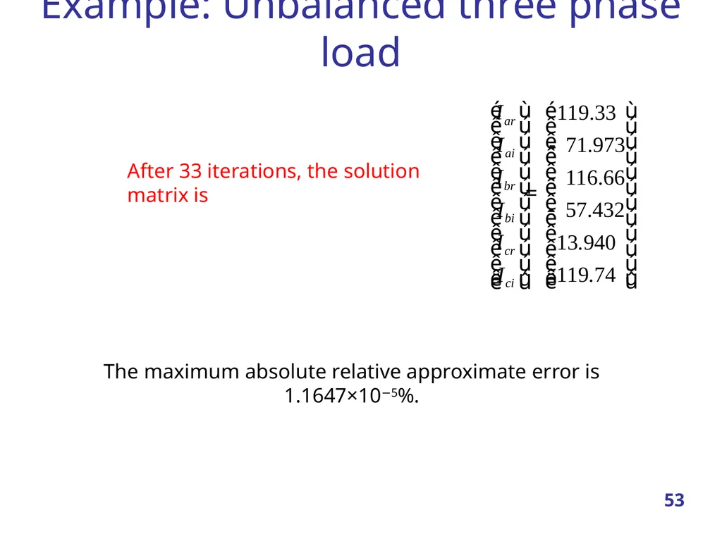
slide53. Example: Unbalanced three phase load After 33 iterations, the solution matrix is The maximum absolute relative approximate error is 1.1647×10⁻⁵%. 53<br>
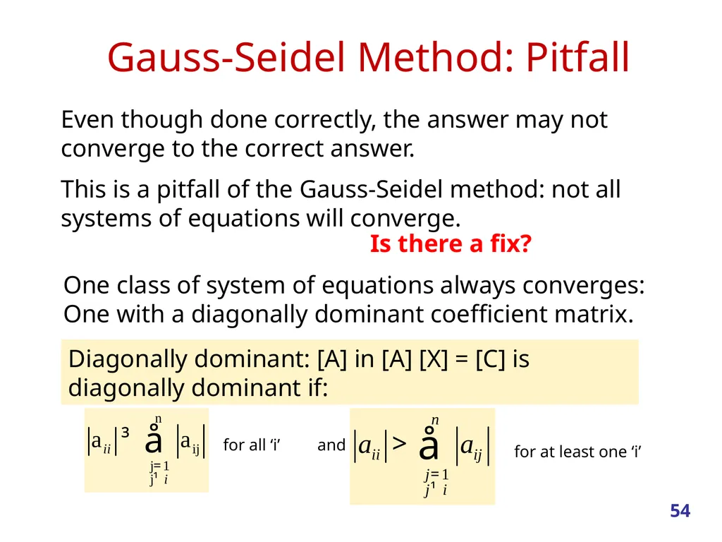
slide54. Gauss-Seidel Method: Pitfall Even though done correctly, the answer may not converge to the correct answer.
This is a pitfall of the Gauss-Seidel method: not all systems of equations will converge. Is there a fix? One class of system of equations always converges: One with a diagonally dominant coefficient matrix. Diagonally dominant: [A] in [A] [X] = [C] is diagonally dominant if: for all ‘i’ and for at least one ‘i’ 54<br>
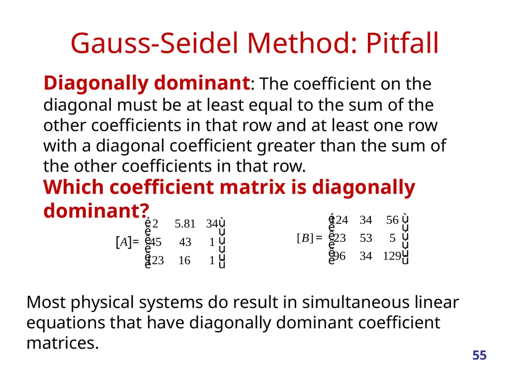
slide55. Gauss-Seidel Method: Pitfall Diagonally dominant: The coefficient on the diagonal must be at least equal to the sum of the other coefficients in that row and at least one row with a diagonal coefficient greater than the sum of the other coefficients in that row. Which coefficient matrix is diagonally dominant? Most physical systems do result in simultaneous linear equations that have diagonally dominant coefficient matrices. 55<br>
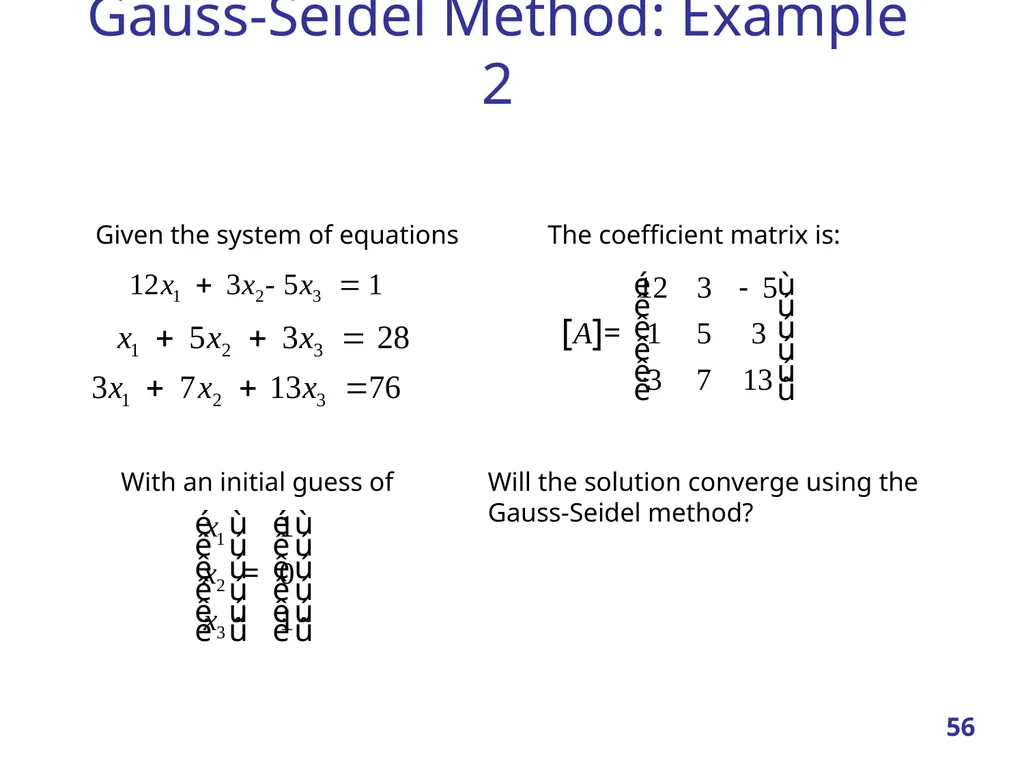
slide56. Gauss-Seidel Method: Example 2 Given the system of equations With an initial guess of The coefficient matrix is: Will the solution converge using the Gauss-Seidel method? 56<br>
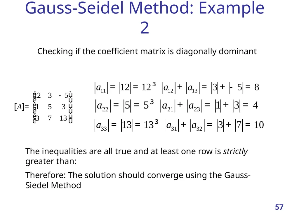
slide57. Gauss-Seidel Method: Example 2 Checking if the coefficient matrix is diagonally dominant The inequalities are all true and at least one row is strictly greater than:
Therefore: The solution should converge using the Gauss-Siedel Method 57<br>
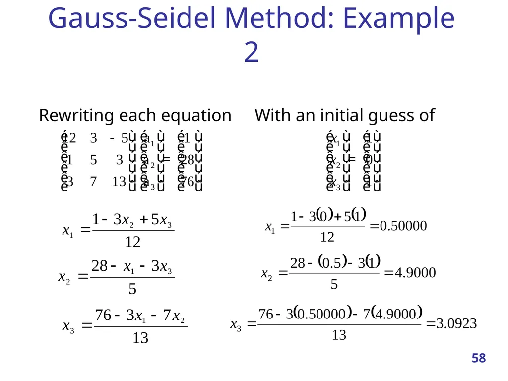
slide58. Gauss-Seidel Method: Example 2 Rewriting each equation With an initial guess of 58<br>
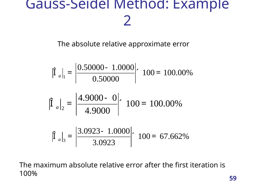
slide59. Gauss-Seidel Method: Example 2 The absolute relative approximate error The maximum absolute relative error after the first iteration is 100% 59<br>
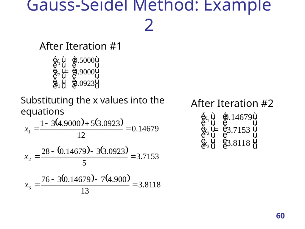
slide60. Gauss-Seidel Method: Example 2 After Iteration #1 Substituting the x values into the equations After Iteration #2 60<br>
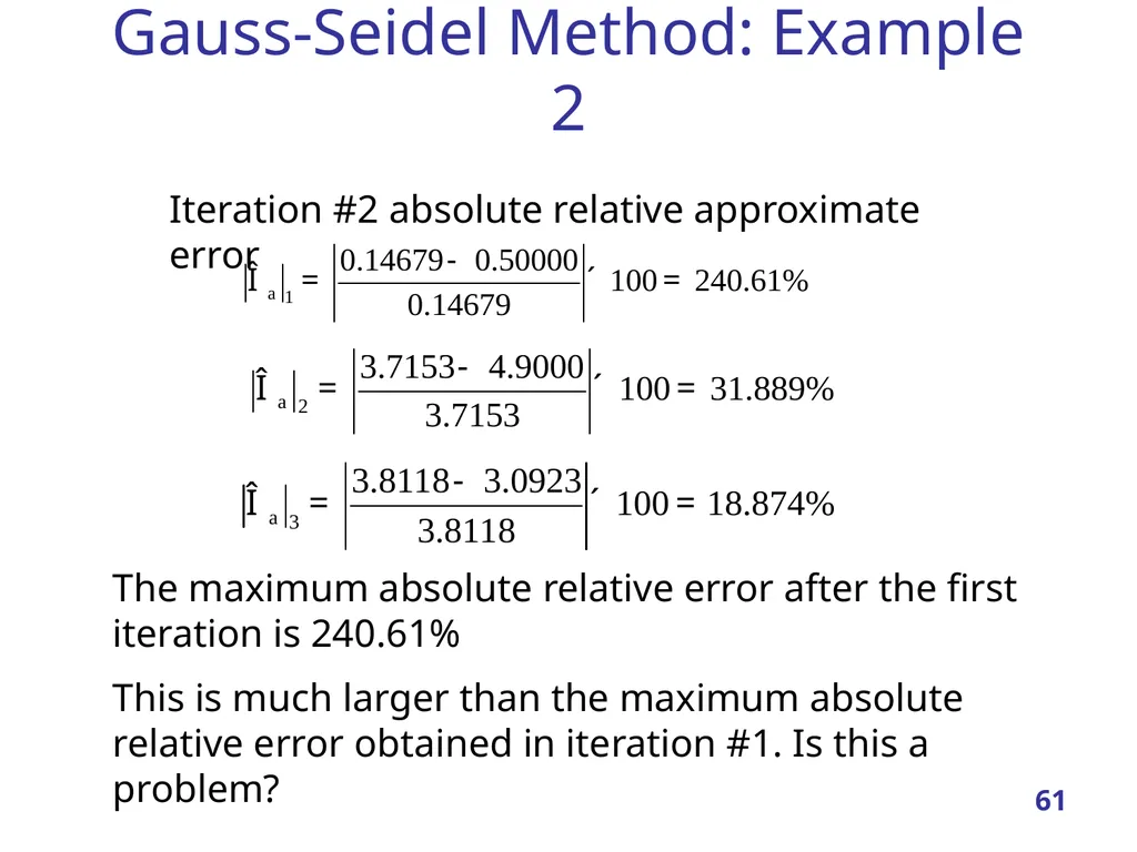
slide61. Gauss-Seidel Method: Example 2 Iteration #2 absolute relative approximate error The maximum absolute relative error after the first iteration is 240.61%
This is much larger than the maximum absolute relative error obtained in iteration #1. Is this a problem? 61<br>
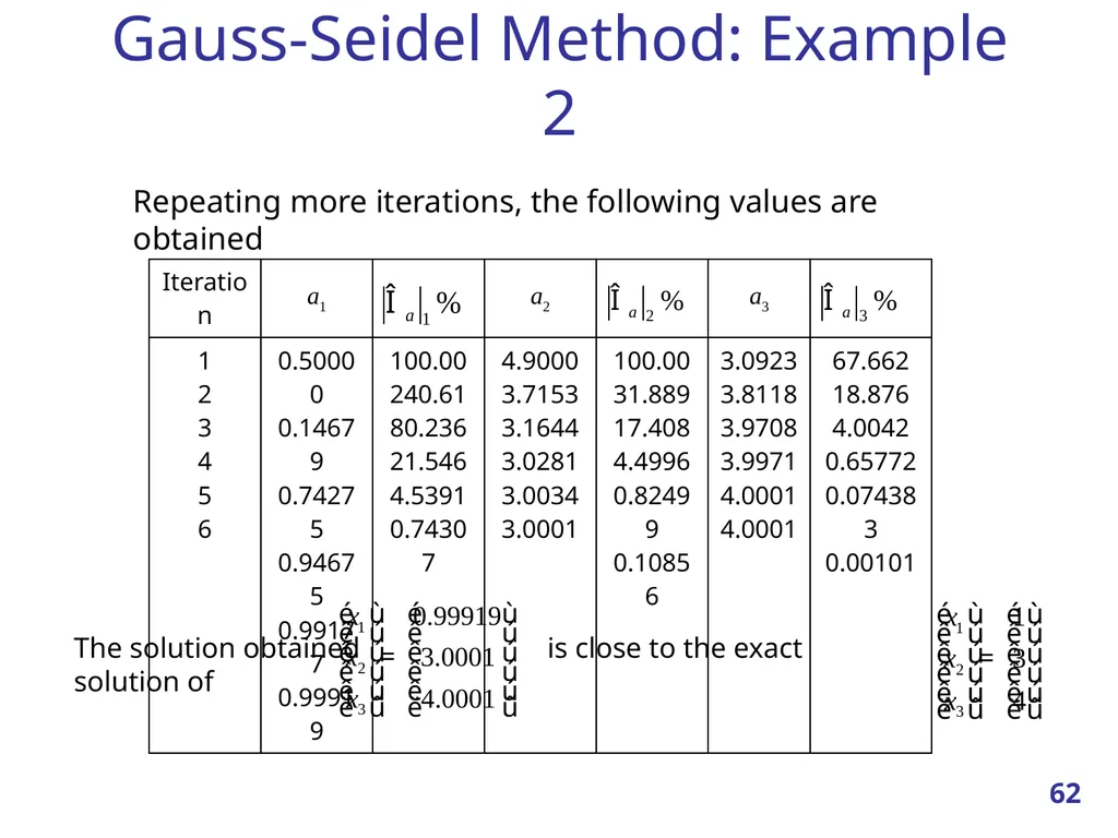
slide62. Gauss-Seidel Method: Example 2 Repeating more iterations, the following values are obtained The solution obtained is close to the exact solution of 62<br>
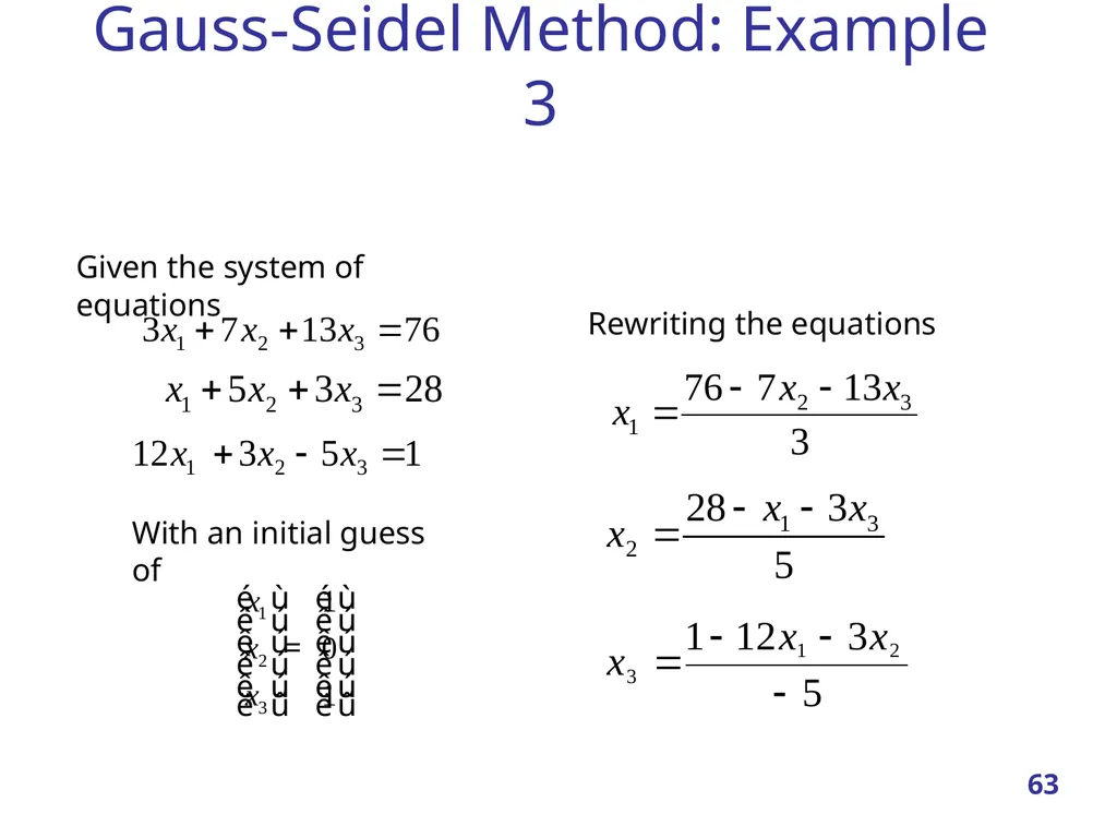
slide63. Gauss-Seidel Method: Example 3 Given the system of equations With an initial guess of Rewriting the equations 63<br>
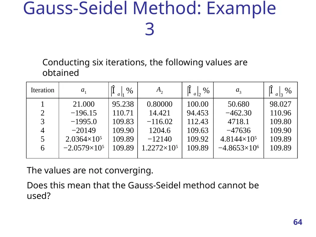
slide64. Gauss-Seidel Method: Example 3 Conducting six iterations, the following values are obtained The values are not converging.
Does this mean that the Gauss-Seidel method cannot be used? 64<br>
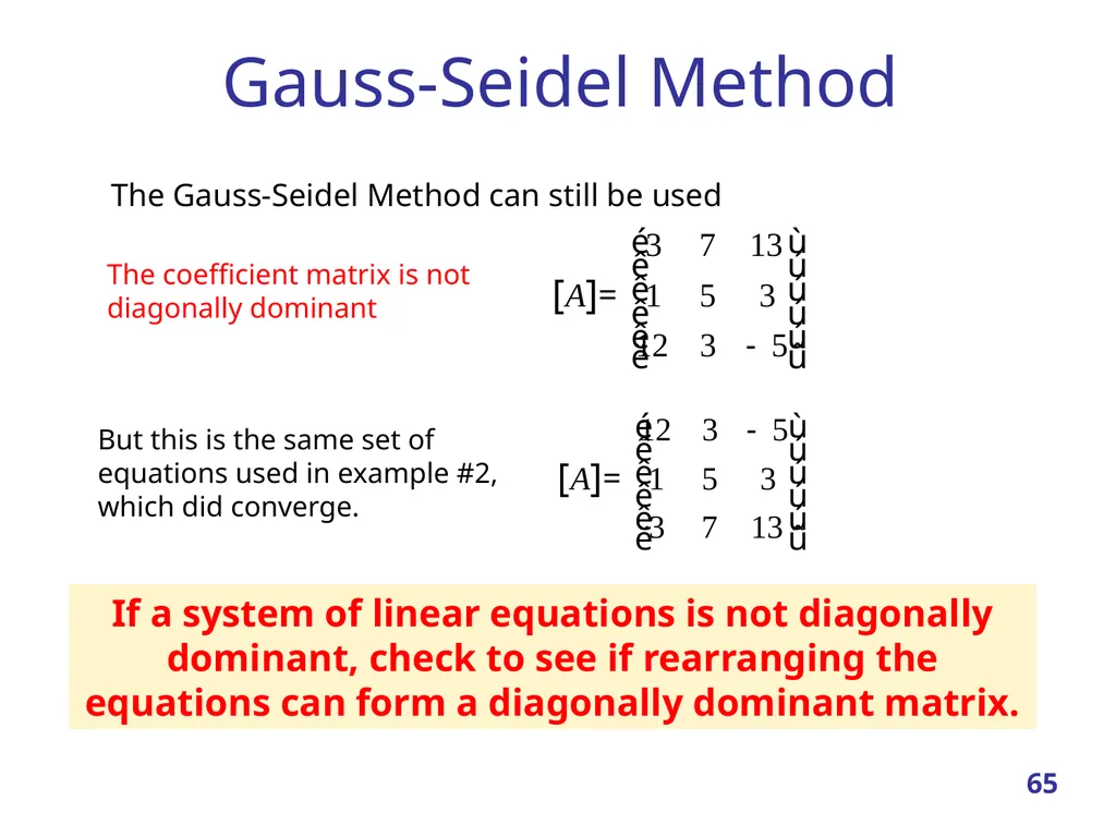
slide65. Gauss-Seidel Method The Gauss-Seidel Method can still be used But this is the same set of equations used in example #2, which did converge. 65 The coefficient matrix is not diagonally dominant If a system of linear equations is not diagonally dominant, check to see if rearranging the equations can form a diagonally dominant matrix.<br>
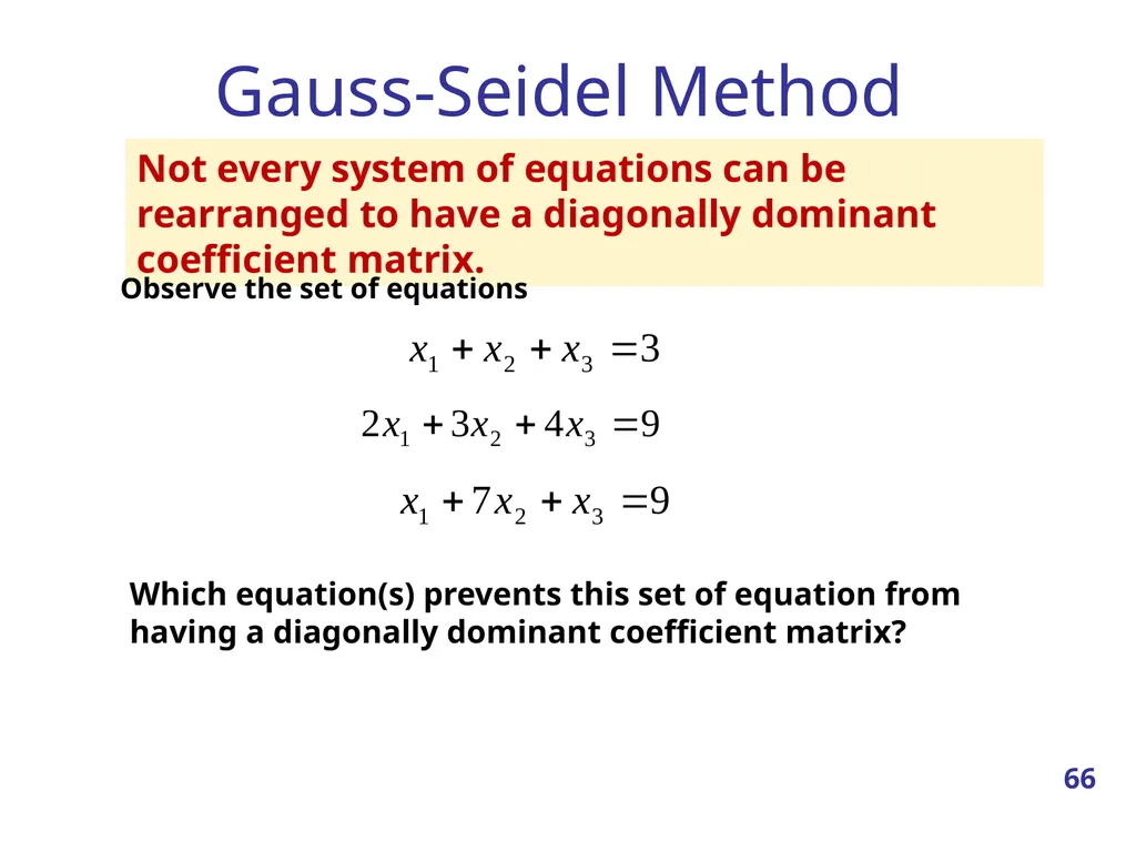
slide66. Gauss-Seidel Method Not every system of equations can be rearranged to have a diagonally dominant coefficient matrix. Observe the set of equations Which equation(s) prevents this set of equation from having a diagonally dominant coefficient matrix? 66<br>
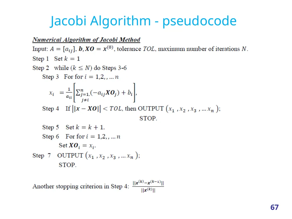
slide67. Jacobi Algorithm - pseudocode 67<br>
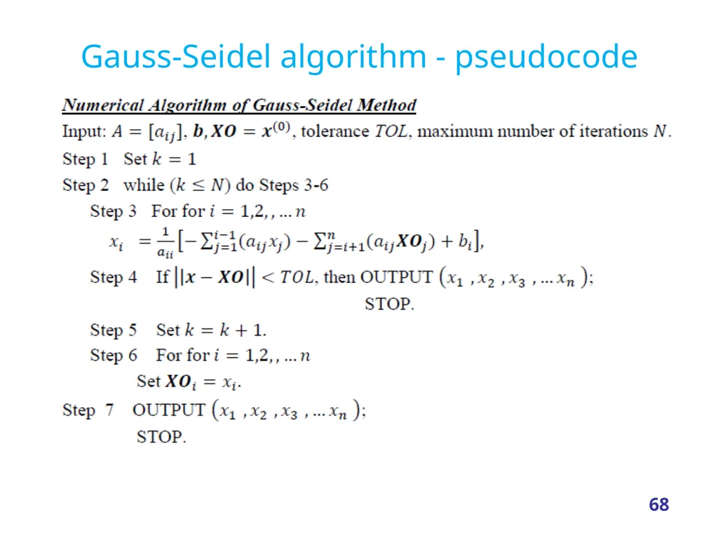
slide68. Gauss-Seidel algorithm - pseudocode 68<br>
slide69. Links 69 https://www.geogebra.org/m/XBKbmXY7 https://www.geogebra.org/m/ekjpgF3z<br>
Gauss-Siedel Method 1<br>
slide2. Iterative Methods Iterative methods can be expressed in the general form: x(k) =F(x(k-1))
where s s.t. F(s)=s is called a Fixed Point
Hopefully: x(k) s (solution of my problem)
Will it converge? How rapidly? 2<br>
slide3. Iterative Methods Stationary:
x(k+1) =Gx(k)+c
where G and c do not depend on iteration count (k)
Non Stationary:
x(k+1) =x(k)+ak p(k)
where computation involves information that change at each iteration 3<br>
slide4. Iterative – Stationary Jacobi In the i-th equation solve for the value of xi while assuming the other entries of x remain fixed:
In matrix terms the method becomes:
where D, L and U represent the diagonal, the strictly lower-trg and strictly upper-trg parts of M 4<br>
slide5. Iterative – Stationary Gauss-Seidel Like Jacobi, but now assume that previously computed results are used as soon as they are available:
In matrix terms the method becomes:
where D, L and U represent the diagonal, the strictly lower-trg and strictly upper-trg parts of M 5<br>
slide6. Iterative – Stationary Successive Overrelaxation (SOR) Devised by extrapolation applied to Gauss-Seidel in the form of weighted average:
In matrix terms the method becomes:
where D, L and U represent the diagonal, the strictly lower-trg and strictly upper-trg parts of M
ω is chosen to increase convergence 6<br>
slide7. 7 Jacobi iteration<br>
slide8. 8 Gauss-Seidel (GS) iteration<br>
slide9. Gauss-Seidel Method An iterative method. Basic Procedure:
Algebraically solve each linear equation for xi
Assume an initial guess solution array
Solve for each xi and repeat
Use absolute relative approximate error after each iteration to check if error is within a pre-specified tolerance. 9<br>
slide10. Gauss-Seidel Method Why? The Gauss-Seidel Method allows the user to control round-off error.
Elimination methods such as Gaussian Elimination and LU Decomposition are prone to prone to round-off error.
Also: If the physics of the problem are understood, a close initial guess can be made, decreasing the number of iterations needed. 10<br>
slide11. Gauss-Seidel Method Algorithm A set of n equations and n unknowns: . .
. .
. . If: the diagonal elements are non-zero
Rewrite each equation solving for the corresponding unknown
ex:
First equation, solve for x1
Second equation, solve for x2 11<br>
slide12. Gauss-Seidel Method Algorithm Rewriting each equation From Equation 1
From equation 2
From equation n-1
From equation n 12<br>
slide13. Gauss-Seidel Method Algorithm General Form of each equation 13<br>
slide14. Gauss-Seidel Method Algorithm General Form for any row ‘i’ How or where can this equation be used? 14<br>
slide15. Gauss-Seidel Method Solve for the unknowns Assume an
initial guess for [X] Use rewritten equations to solve for each value of xi.
Important: Remember to use the most recent value of xi. Which means to apply values calculated to the calculations remaining in the current iteration. 15<br>
slide16. Gauss-Seidel Method Calculate the Absolute Relative Approximate Error So when has the answer been found?
The iterations are stopped when the absolute relative approximate error is less than a prespecified tolerance for all unknowns. 16<br>
slide17. 17 Suppose that for conciseness we limit ourselves to a 3X3 set of equations. where j and j -1 are the present and previous iterations.
To start the solution process, initial guesses must be made for the x’s. A simple approach is to assume that they are all zero.<br>
slide18. 18 Convergence can be checked using the criterion that for i,<br>
slide19. 19 Graphical depiction of the difference between (a) the Gauss-Seidel and (b) the Jacobi iterative methods for solving simultaneous linear algebraic equations.<br>
slide20. Jacobi's Method 20 https://www.maa.org/press/periodicals/loci/joma/iterative-methods-for-solving-iaxi-ibi-jacobis-method Perhaps the simplest iterative method for solving Ax=b is Jacobi’s Method.
Note that the simplicity of this method is both good and bad:
good, because it is relatively easy to understand and thus is a good first taste of iterative methods;
bad, because it is not typically used in practice (although its potential usefulness has been reconsidered with the advent of parallel computing).
Still, it is a good starting point for learning about more useful, but more complicated, iterative methods.<br>
slide21. Jacobi Iterative Technique Consider the following set of equations. 21<br>
slide22. Convert the set Ax = b in the form of x = Tx + c. 22<br>
slide23. Start with an initial approximation of: 23<br>
slide24. 24<br>
slide25. 25<br>
slide26. 26<br>
slide27. Results of Jacobi Iteration: 27<br>
slide28. Gauss-Seidel Iterative Technique Consider the following set of equations. 28<br>
slide29. 29<br>
slide30. 30<br>
slide31. Results of Gauss-Seidel Iteration:
(Blue numbers are for Jacobi iterations.) 31<br>
slide32. It required 15 iterations for Jacobi method and 7 iterations for Gauss-Seidel method to arrive at the solution with a tolerance of 0.00001.
While Jacobi would usually be the slowest of the iterative methods, it is well suited to illustrate an algorithm that is well suited for parallel processing!!! The solution is: x1= 1, x2 = 2, x3 = -1, x4 = 1 32<br>
slide33. 33 EXAMPLE Gauss-Seidel Method
Problem Statement. Use the Gauss-Seidel method to obtain the solution for Note that the solution is Solution. First, solve each of the equations for its unknown on the diagonal:<br>
slide34. 34 By assuming that x2 and x3 are zero This value, along with the assumed value of x3 =0, can be substituted into Eq.(2) to calculate<br>
slide35. 35 The first iteration is completed by substituting the calculated values for x1 and x2 into Eq.(3) to yield For the second iteration, the same process is repeated to compute<br>
slide36. 36 The method is, therefore, converging on the true solution. Additional iterations could be applied to improve the answers. Consequently, we can estimate the error. For example , for x1 For x2 and x3 , the error estimates are Repeat to it again until the result is known to at least the tolerance specified by<br>
slide37. Example: Unbalanced three phase load Three-phase loads are common in AC systems. When the system is balanced the analysis can be simplified to a single equivalent circuit model. However, when it is unbalanced the only practical solution involves the solution of simultaneous linear equations. In a model the following equations need to be solved. Find the values of Iar , Iai , Ibr , Ibi , Icr , and Ici using the Gauss-Seidel method. 37<br>
slide38. Example: Unbalanced three phase load Rewrite each equation to solve for each of the unknowns 38<br>
slide39. Example: Unbalanced three phase load Initial Guess: For iteration 1, start with an initial guess value 39<br>
slide40. Example: Unbalanced three phase load Substituting the guess values into the first equation Substituting the new value of Iar and the remaining guess values into
the second equation 40<br>
slide41. Example: Unbalanced three phase load Substituting the new values Iar , Iai , and the remaining guess values into
the third equation Substituting the new values Iar , Iai , Ibr , and the remaining guess values into
the fourth equation 41<br>
slide42. Example: Unbalanced three phase load Substituting the new values Iar , Iai , Ibr , Ibi , and the remaining guess values into the fifth equation Substituting the new values Iar , Iai , Ibr , Ibi , Icr , and the remaining guess value into the sixth equation 42<br>
slide43. Example: Unbalanced three phase load How accurate is the solution? Find the absolute relative approximate error using: At the end of the first iteration, the solution matrix is: 43<br>
slide44. Example: Unbalanced three phase load Calculating the absolute relative approximate errors The maximum error after the first iteration is:
131.98%
Another iteration is needed! 44<br>
slide45. Example: Unbalanced three phase load Starting with the values obtained in iteration #1 Substituting the values from Iteration 1 into the first equation 45<br>
slide46. Example: Unbalanced three phase load Substituting the new value of Iar and the remaining values from
Iteration 1 into the second equation Substituting the new values Iar , Iai , and the remaining values from
Iteration 1 into the third equation 46<br>
slide47. Example: Unbalanced three phase load Substituting the new values Iar , Iai , Ibr , and the remaining values from
Iteration 1 into the fourth equation Substituting the new values Iar , Iai , Ibr , Ibi , and the remaining values
From Iteration 1 into the fifth equation 47<br>
slide48. Example: Unbalanced three phase load Substituting the new values Iar , Iai , Ibr , Ibi , Icr , and the remaining
value from Iteration 1 into the sixth equation The solution matrix at the end of the second iteration is: 48<br>
slide49. Example: Unbalanced three phase load Calculating the absolute relative approximate errors for the second iteration The maximum error after the second iteration is:
209.24%
More iterations are needed! 49<br>
slide50. Example: Unbalanced three phase load Repeating more iterations, the following values are obtained 50<br>
slide51. Example: Unbalanced three phase load The absolute relative approximate error is still high, but allowing for more iterations, the error quickly begins to converge to zero.
What could have been done differently to allow for a faster convergence? After six iterations, the solution matrix is The maximum error after the sixth iteration is:
65.729% 51<br>
slide52. Example: Unbalanced three phase load Repeating more iterations, the following values are obtained 52<br>
slide53. Example: Unbalanced three phase load After 33 iterations, the solution matrix is The maximum absolute relative approximate error is 1.1647×10⁻⁵%. 53<br>
slide54. Gauss-Seidel Method: Pitfall Even though done correctly, the answer may not converge to the correct answer.
This is a pitfall of the Gauss-Seidel method: not all systems of equations will converge. Is there a fix? One class of system of equations always converges: One with a diagonally dominant coefficient matrix. Diagonally dominant: [A] in [A] [X] = [C] is diagonally dominant if: for all ‘i’ and for at least one ‘i’ 54<br>
slide55. Gauss-Seidel Method: Pitfall Diagonally dominant: The coefficient on the diagonal must be at least equal to the sum of the other coefficients in that row and at least one row with a diagonal coefficient greater than the sum of the other coefficients in that row. Which coefficient matrix is diagonally dominant? Most physical systems do result in simultaneous linear equations that have diagonally dominant coefficient matrices. 55<br>
slide56. Gauss-Seidel Method: Example 2 Given the system of equations With an initial guess of The coefficient matrix is: Will the solution converge using the Gauss-Seidel method? 56<br>
slide57. Gauss-Seidel Method: Example 2 Checking if the coefficient matrix is diagonally dominant The inequalities are all true and at least one row is strictly greater than:
Therefore: The solution should converge using the Gauss-Siedel Method 57<br>
slide58. Gauss-Seidel Method: Example 2 Rewriting each equation With an initial guess of 58<br>
slide59. Gauss-Seidel Method: Example 2 The absolute relative approximate error The maximum absolute relative error after the first iteration is 100% 59<br>
slide60. Gauss-Seidel Method: Example 2 After Iteration #1 Substituting the x values into the equations After Iteration #2 60<br>
slide61. Gauss-Seidel Method: Example 2 Iteration #2 absolute relative approximate error The maximum absolute relative error after the first iteration is 240.61%
This is much larger than the maximum absolute relative error obtained in iteration #1. Is this a problem? 61<br>
slide62. Gauss-Seidel Method: Example 2 Repeating more iterations, the following values are obtained The solution obtained is close to the exact solution of 62<br>
slide63. Gauss-Seidel Method: Example 3 Given the system of equations With an initial guess of Rewriting the equations 63<br>
slide64. Gauss-Seidel Method: Example 3 Conducting six iterations, the following values are obtained The values are not converging.
Does this mean that the Gauss-Seidel method cannot be used? 64<br>
slide65. Gauss-Seidel Method The Gauss-Seidel Method can still be used But this is the same set of equations used in example #2, which did converge. 65 The coefficient matrix is not diagonally dominant If a system of linear equations is not diagonally dominant, check to see if rearranging the equations can form a diagonally dominant matrix.<br>
slide66. Gauss-Seidel Method Not every system of equations can be rearranged to have a diagonally dominant coefficient matrix. Observe the set of equations Which equation(s) prevents this set of equation from having a diagonally dominant coefficient matrix? 66<br>
slide67. Jacobi Algorithm - pseudocode 67<br>
slide68. Gauss-Seidel algorithm - pseudocode 68<br>
slide69. Links 69 https://www.geogebra.org/m/XBKbmXY7 https://www.geogebra.org/m/ekjpgF3z<br>