
Machine Learning is Better – But When? Keith Ord



Description: Machine Learning is Better But When? Keith Ord Professor Emeritus of Business Statistics When? A recent study by Efron (2020) provides a detailed assessment of the strengths and weaknesses of traditional regression-type methods and pure
Related Topics
Download Presentation
"Machine Learning is Better – But When? Keith Ord" is the property of its rightful owner. Permission is granted to download and print the materials on this website for personal, non-commercial use only, and to display it on your personal computer provided you do not modify the materials and that you retain all copyright notices contained in the materials. By downloading content from our website, you accept the terms of this agreement.
Presentation Transcript
slide1. Machine Learning is Better – But When? Keith Ord
Professor Emeritus of Business Statistics<br>
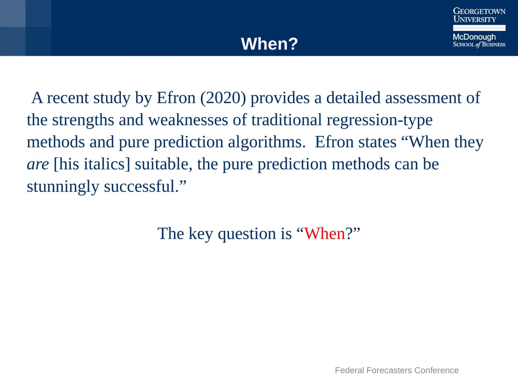
slide2. When? A recent study by Efron (2020) provides a detailed assessment of the strengths and weaknesses of traditional regression-type methods and pure prediction algorithms. Efron states “When they are [his italics] suitable, the pure prediction methods can be stunningly successful.”
The key question is “When?” 9/9/2222/229/21/2022 Federal Forecasters Conference 2<br>
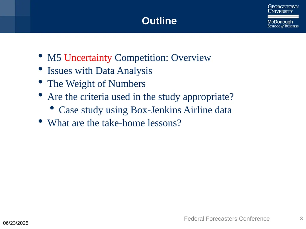
slide3. Outline M5 Uncertainty Competition: Overview
Issues with Data Analysis
The Weight of Numbers
Are the criteria used in the study appropriate?
Case study using Box-Jenkins Airline data
What are the take-home lessons? 9/21/2022 Federal Forecasters Conference 3<br>
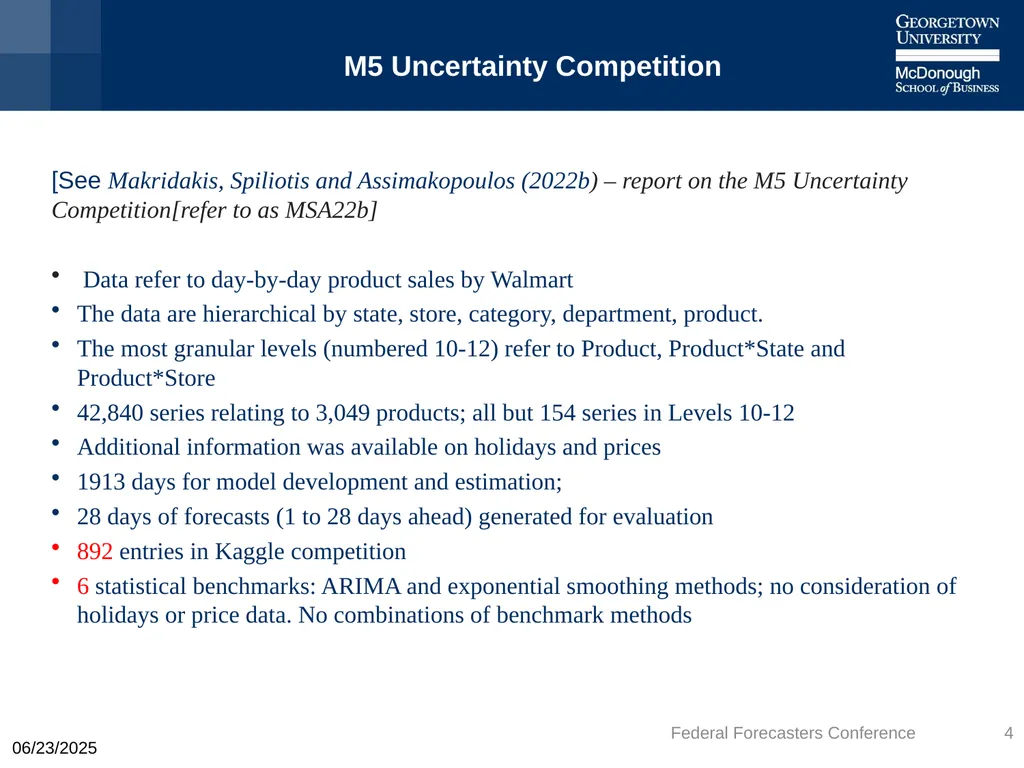
slide4. M5 Uncertainty Competition [See Makridakis, Spiliotis and Assimakopoulos (2022b) – report on the M5 Uncertainty Competition[refer to as MSA22b]
Data refer to day-by-day product sales by Walmart
The data are hierarchical by state, store, category, department, product.
The most granular levels (numbered 10-12) refer to Product, Product*State and Product*Store
42,840 series relating to 3,049 products; all but 154 series in Levels 10-12
Additional information was available on holidays and prices
1913 days for model development and estimation;
28 days of forecasts (1 to 28 days ahead) generated for evaluation
892 entries in Kaggle competition
6 statistical benchmarks: ARIMA and exponential smoothing methods; no consideration of holidays or price data. No combinations of benchmark methods 9/21/2022 Federal Forecasters Conference 4<br>
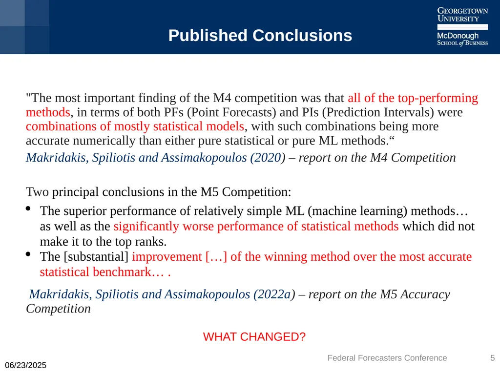
slide5. Published Conclusions "The most important finding of the M4 competition was that all of the top-performing methods, in terms of both PFs (Point Forecasts) and PIs (Prediction Intervals) were combinations of mostly statistical models, with such combinations being more accurate numerically than either pure statistical or pure ML methods.“
Makridakis, Spiliotis and Assimakopoulos (2020) – report on the M4 Competition
Two principal conclusions in the M5 Competition:
The superior performance of relatively simple ML (machine learning) methods… as well as the significantly worse performance of statistical methods which did not make it to the top ranks.
The [substantial] improvement […] of the winning method over the most accurate statistical benchmark… .
Makridakis, Spiliotis and Assimakopoulos (2022a) – report on the M5 Accuracy Competition
WHAT CHANGED? 9/21/2022 Federal Forecasters Conference 5<br>
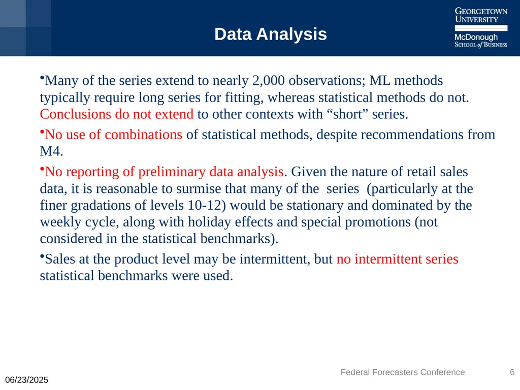
slide6. Data Analysis Many of the series extend to nearly 2,000 observations; ML methods typically require long series for fitting, whereas statistical methods do not. Conclusions do not extend to other contexts with “short” series.
No use of combinations of statistical methods, despite recommendations from M4.
No reporting of preliminary data analysis. Given the nature of retail sales data, it is reasonable to surmise that many of the series (particularly at the finer gradations of levels 10-12) would be stationary and dominated by the weekly cycle, along with holiday effects and special promotions (not considered in the statistical benchmarks).
Sales at the product level may be intermittent, but no intermittent series statistical benchmarks were used. 9/21/2022 Federal Forecasters Conference 6<br>
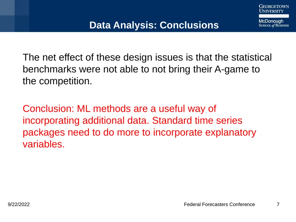
slide7. Data Analysis: Conclusions The net effect of these design issues is that the statistical benchmarks were not able to not bring their A-game to the competition.
Conclusion: ML methods are a useful way of incorporating additional data. Standard time series packages need to do more to incorporate explanatory variables. 7 9/22/2022 Federal Forecasters Conference 7<br>
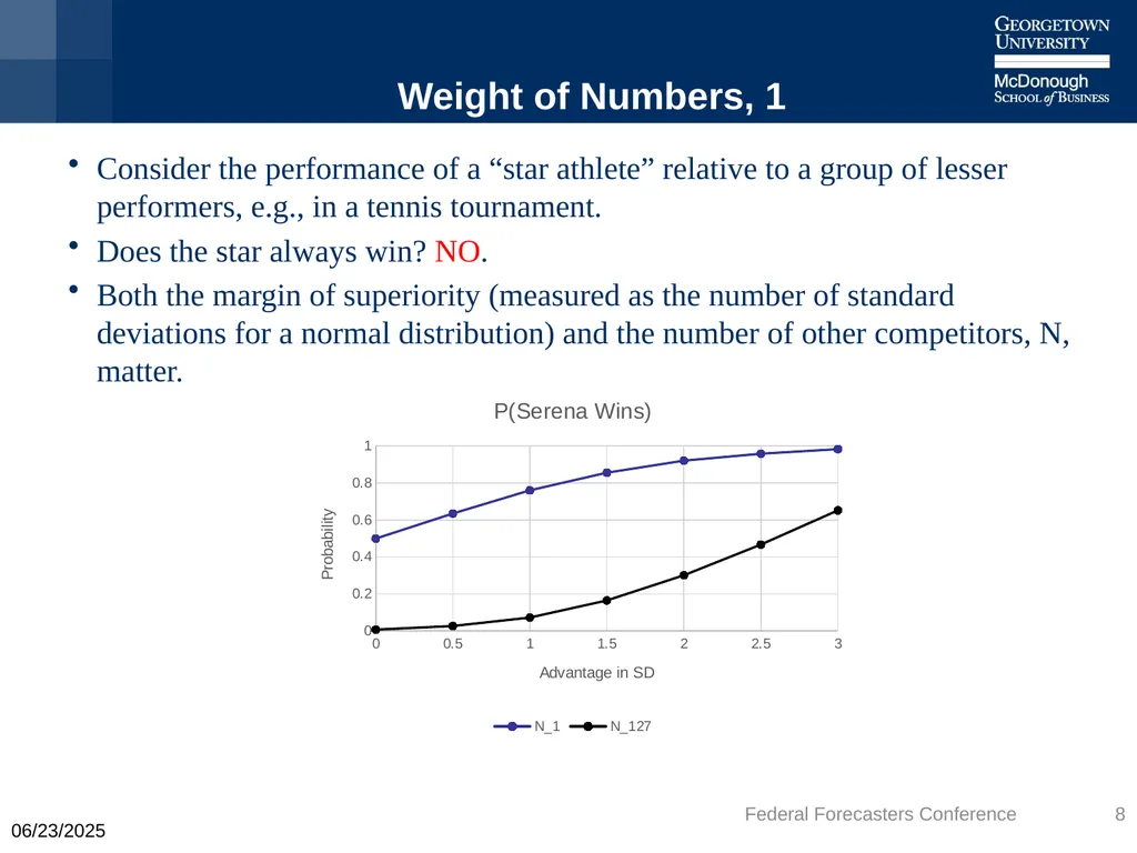
slide8. Weight of Numbers, 1 Consider the performance of a “star athlete” relative to a group of lesser performers, e.g., in a tennis tournament.
Does the star always win? NO.
Both the margin of superiority (measured as the number of standard deviations for a normal distribution) and the number of other competitors, N, matter. 9/21/2022 Federal Forecasters Conference 8<br>
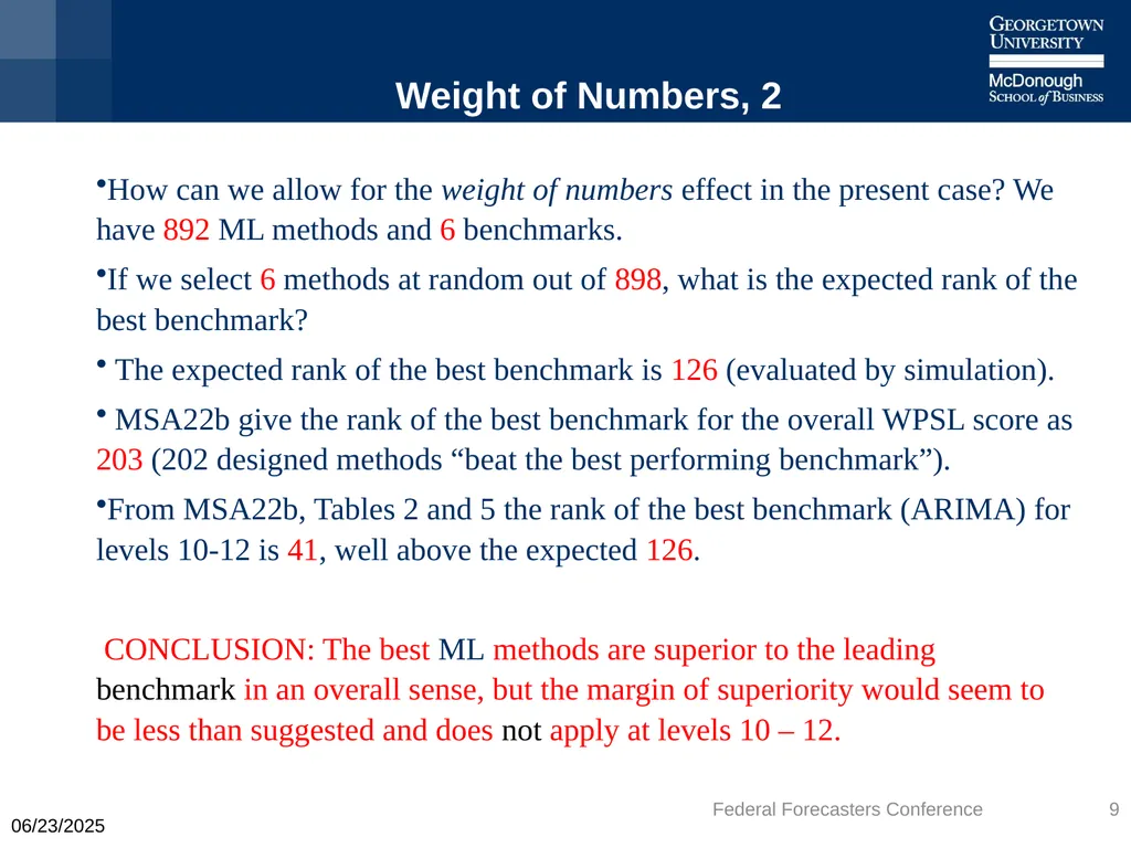
slide9. Weight of Numbers, 2 How can we allow for the weight of numbers effect in the present case? We have 892 ML methods and 6 benchmarks.
If we select 6 methods at random out of 898, what is the expected rank of the best benchmark?
The expected rank of the best benchmark is 126 (evaluated by simulation).
MSA22b give the rank of the best benchmark for the overall WPSL score as 203 (202 designed methods “beat the best performing benchmark”).
From MSA22b, Tables 2 and 5 the rank of the best benchmark (ARIMA) for levels 10-12 is 41, well above the expected 126.
CONCLUSION: The best ML methods are superior to the leading benchmark in an overall sense, but the margin of superiority would seem to be less than suggested and does not apply at levels 10 – 12. 9/21/2022 Federal Forecasters Conference 9<br>
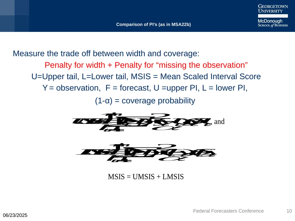
slide10. Comparison of PI’s (as in MSA22b) Measure the trade off between width and coverage:
Penalty for width + Penalty for “missing the observation”
U=Upper tail, L=Lower tail, MSIS = Mean Scaled Interval Score
Y = observation, F = forecast, U =upper PI, L = lower PI,
(1-α) = coverage probability Federal Forecasters Conference 10 9/21/2022<br>
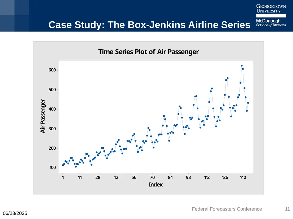
slide11. Case Study: The Box-Jenkins Airline Series 9/21/2022 Federal Forecasters Conference 11<br>
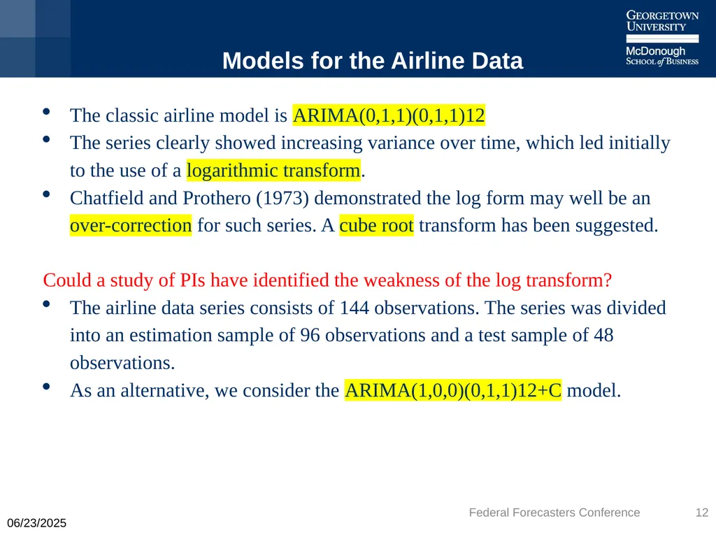
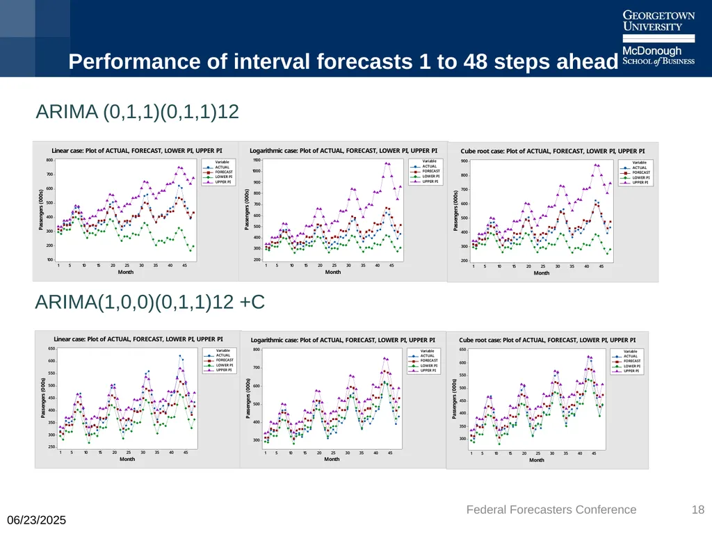
slide12. Models for the Airline Data The classic airline model is ARIMA(0,1,1)(0,1,1)12
The series clearly showed increasing variance over time, which led initially to the use of a logarithmic transform.
Chatfield and Prothero (1973) demonstrated the log form may well be an over-correction for such series. A cube root transform has been suggested.
Could a study of PIs have identified the weakness of the log transform?
The airline data series consists of 144 observations. The series was divided into an estimation sample of 96 observations and a test sample of 48 observations.
As an alternative, we consider the ARIMA(1,0,0)(0,1,1)12+C model. 9/21/2022 Federal Forecasters Conference 12<br>
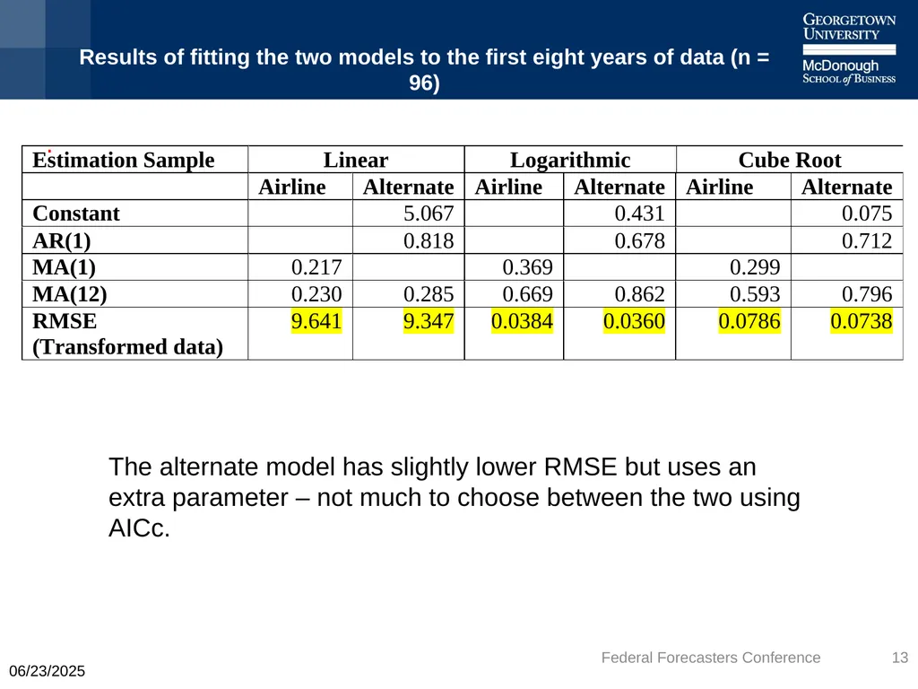
slide13. Results of fitting the two models to the first eight years of data (n = 96) . 9/21/2022 Federal Forecasters Conference 13 The alternate model has slightly lower RMSE but uses an extra parameter – not much to choose between the two using AICc.<br>
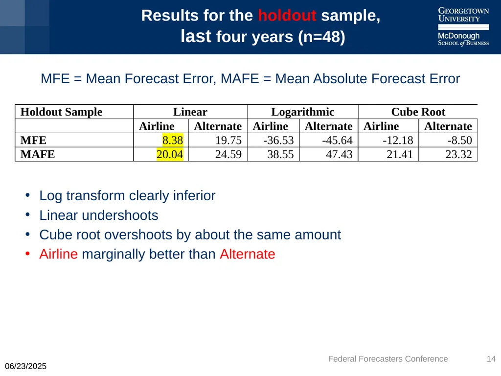
slide14. Results for the holdout sample, last four years (n=48) MFE = Mean Forecast Error, MAFE = Mean Absolute Forecast Error
Log transform clearly inferior
Linear undershoots
Cube root overshoots by about the same amount
Airline marginally better than Alternate 9/21/2022 Federal Forecasters Conference 14<br>
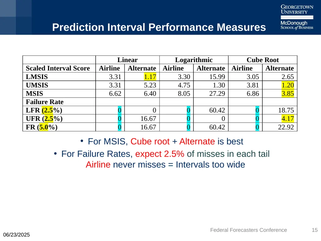
slide15. Prediction Interval Performance Measures 9/21/2022 Federal Forecasters Conference 15 For MSIS, Cube root + Alternate is best
For Failure Rates, expect 2.5% of misses in each tail Airline never misses = Intervals too wide<br>
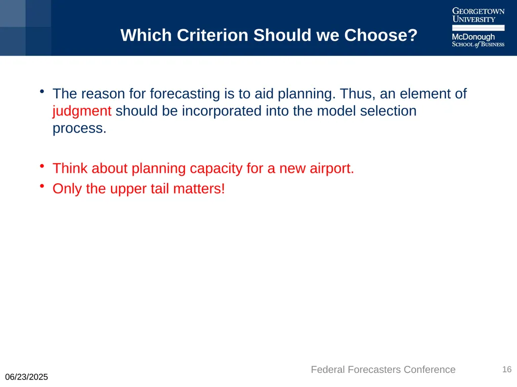
slide16. Which Criterion Should we Choose? The reason for forecasting is to aid planning. Thus, an element of judgment should be incorporated into the model selection process.
Think about planning capacity for a new airport.
Only the upper tail matters! 9/21/2022 Federal Forecasters Conference 16<br>
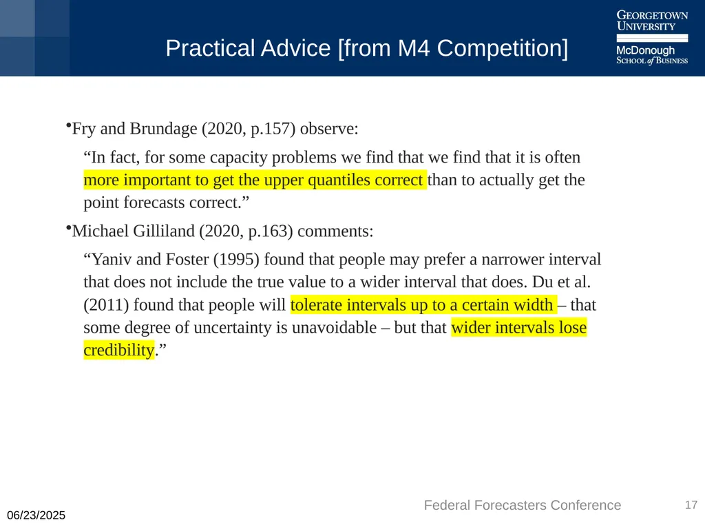
slide17. Practical Advice [from M4 Competition] Fry and Brundage (2020, p.157) observe:
“In fact, for some capacity problems we find that we find that it is often more important to get the upper quantiles correct than to actually get the point forecasts correct.”
Michael Gilliland (2020, p.163) comments:
“Yaniv and Foster (1995) found that people may prefer a narrower interval that does not include the true value to a wider interval that does. Du et al. (2011) found that people will tolerate intervals up to a certain width – that some degree of uncertainty is unavoidable – but that wider intervals lose credibility.” 9/21/2022 Federal Forecasters Conference 17<br>
slide18. Performance of interval forecasts 1 to 48 steps ahead ARIMA (0,1,1)(0,1,1)12 9/21/2022 Federal Forecasters Conference 18 ARIMA(1,0,0)(0,1,1)12 +C<br>
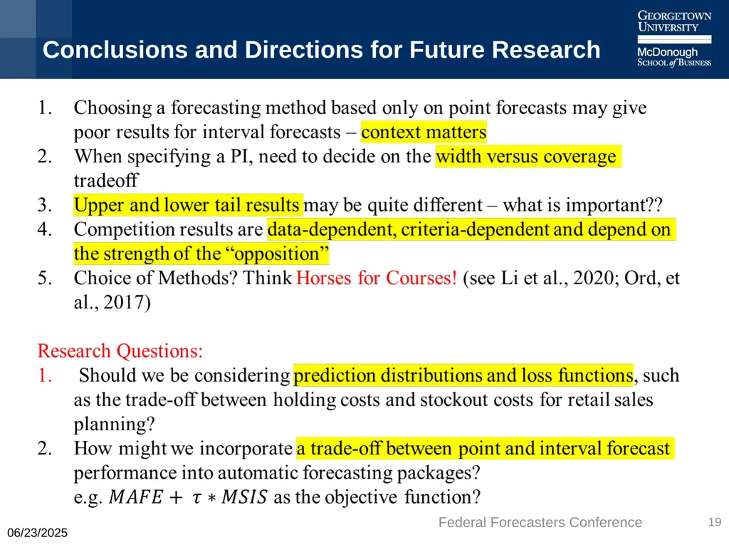
slide19. Conclusions and Directions for Future Research 9/21/2022 Federal Forecasters Conference 19<br>
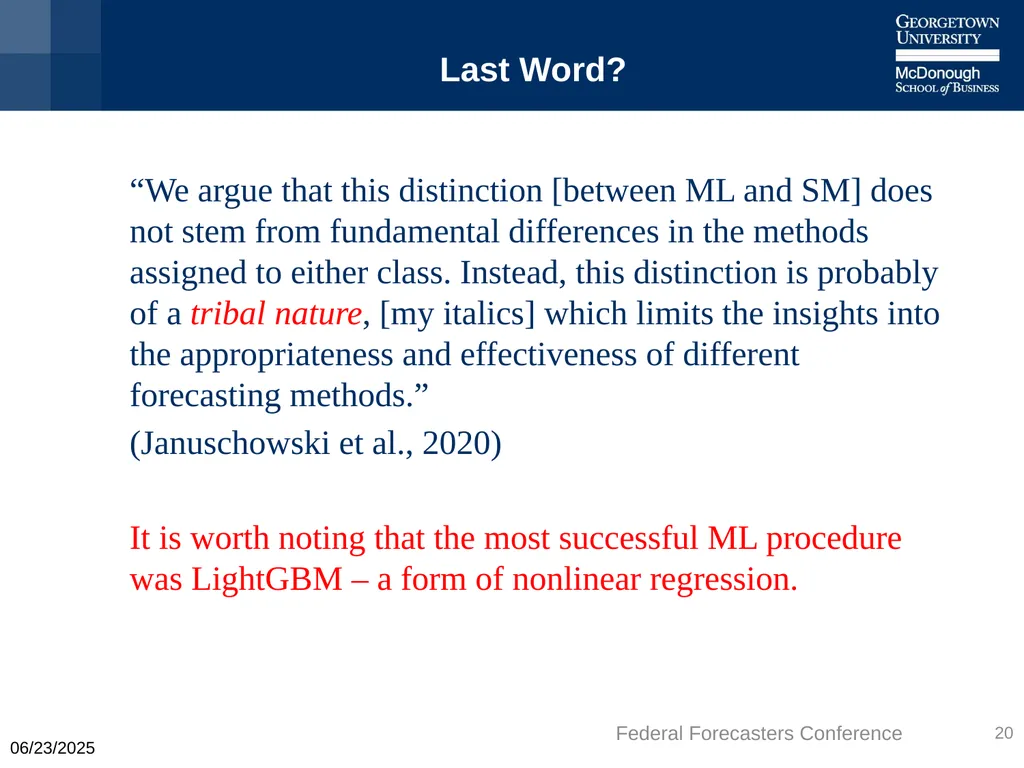
slide20. Last Word? “We argue that this distinction [between ML and SM] does not stem from fundamental differences in the methods assigned to either class. Instead, this distinction is probably of a tribal nature, [my italics] which limits the insights into the appropriateness and effectiveness of different forecasting methods.”
(Januschowski et al., 2020)
It is worth noting that the most successful ML procedure was LightGBM – a form of nonlinear regression. 9/21/2022 Federal Forecasters Conference 20<br>
slide21. . SO, WHEN??
THANK YOU! 9/21/2022 Federal Forecasters Conference 21<br>
slide22. References Chatfield, C. (1993). Calculating interval forecasts. Journal of Business and Economic Statistics, 11, 121-135.
Du, N., Budesco, D., Shelly, M. & Omer, T. (2011). The appeal of vague financial forecasts. Organizational Behavior and Human Decision Processes, 114, 179-189
Efron. B. (2020). Prediction, Estimation and Attribution. Journal of the American Statistical Association, 115, 636-655.
Fry, C. & Brundage, M. (2020). The M4 forecasting competition – A practitioner’s view. International Journal of Forecasting, 36, 157-160.
Gilliland, M. (2020). The value added by machine learning approaches in forecasting. International Journal of Forecasting, 36, 161-166.
Januschowski, T., Gashaus, J., Wang, Y., Salinas, D., Flunkert, V., Bohlke-Schneider, M. and Callot, L. (2020). Criteria for classifying forecasting methods. International Journal of Forecasting, 36, 167-177
Li, Y., Berry, D., & Lee, J. (2020) How to choose among three forecasting methods. Foresight, Issue 58, 7 – 14.
Makridakis, S., Spiliotis, E. & Assimakopoulos, V. (2020). The M4 Competition: 100,000 time series and 61 forecasting methods. International Journal of Forecasting, 36, 54 – 74.
Makridakis, S., Spiliotis, E. & Assimakopoulos, V. (2022a). The M5 Accuracy Competition: Results, Findings and Conclusions. International Journal of Forecasting, to appear.
Makridakis, S., Spiliotis, E. & Assimakopoulos, V. (2022b). The M5 Uncertainty Competition: Results, Findings and Conclusions. International Journal of Forecasting, to appear.
Ord, K., Fildes, R. & Kourentzes, N. (2017). Principles of Business Forecasting. New York:Wessex Press. 2nd edition.
Yaniv, L. & Foster, D. (1995). Graininess of judgment under uncertainty: An accuracy-awareness tradeoff. Journal of Experimental Psychology: General, 124(4), 424-432 9/21/2022 Federal Forecasters Conference 22<br>
slide23. ML and SM Methods The Kaggle platform brought a welcome infusion of computer scientists into the competition and the quality of ML methods used in M5 represents a considerable improvement over M4. But are the conclusions presented in MSA21 reasonable?
ML methods are often based upon statistical methodologies. For example, MSA21 refers to LightGBM as “a ML algorithm for performing non-linear regression using gradient boosted trees,” and neural net methods build upon logistic regression and multilevel structures.
What is new is the computing power now available to develop large-scale models involving multiple series, and to search for nonlinear structure. 9/21/2022 Federal Forecasters Conference 23<br>
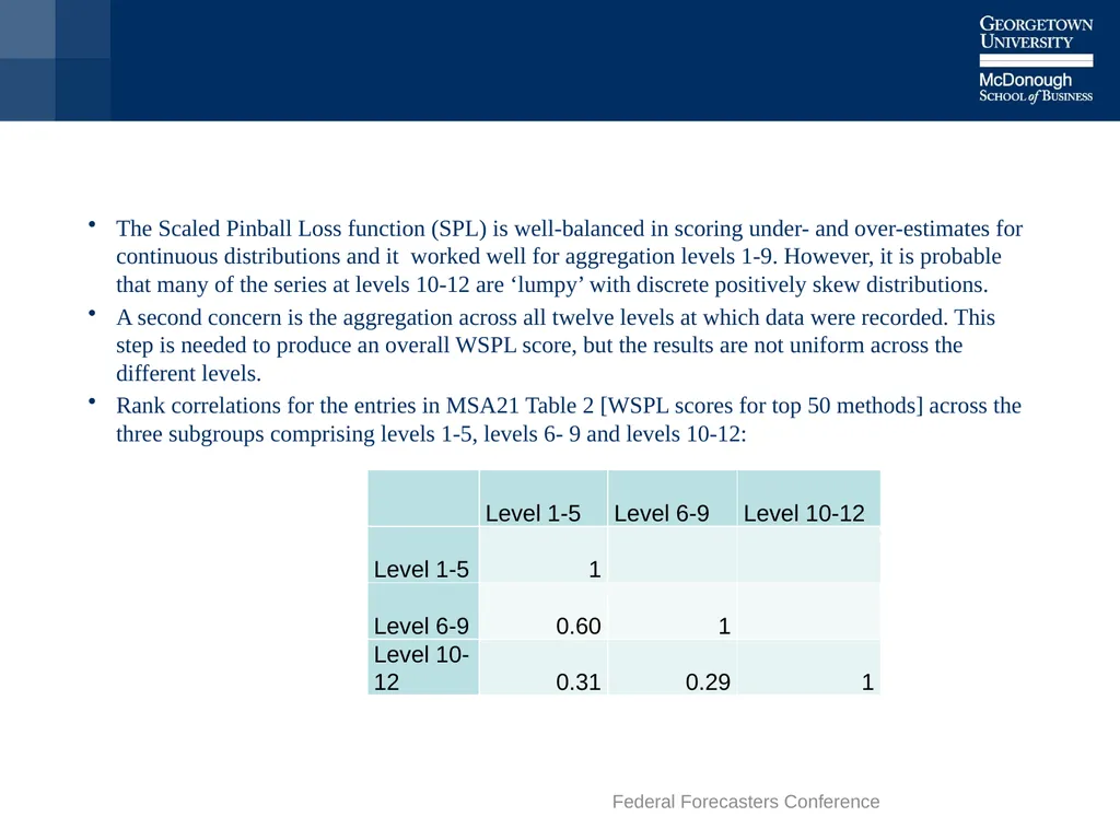
slide24. Choice of Criteria The Scaled Pinball Loss function (SPL) is well-balanced in scoring under- and over-estimates for continuous distributions and it worked well for aggregation levels 1-9. However, it is probable that many of the series at levels 10-12 are ‘lumpy’ with discrete positively skew distributions.
A second concern is the aggregation across all twelve levels at which data were recorded. This step is needed to produce an overall WSPL score, but the results are not uniform across the different levels.
Rank correlations for the entries in MSA21 Table 2 [WSPL scores for top 50 methods] across the three subgroups comprising levels 1-5, levels 6- 9 and levels 10-12: 9/21/2022 Federal Forecasters Conference 24<br>
slide25. What can statistical modelers learn going forward? The superiority of relatively simple methods is reaffirmed, although the statement should perhaps be more nuanced: Don’t use methods that are beyond what the data can bear. The present study uses a large information set about 2,000x30,000=60 million data points, which will not be available in many applications.
How long a series is needed to sustain a particular method remains an important practical question.
The importance of explanatory variables depends both on the context and on the forecaster’s objectives. If the focus is on policy evaluation, key variables must factor into the analysis. Likewise, calendar and pricing variables may be important for policy purposes. Forecasting software needs to improve the ability to incorporate such effects.
The question of compatible interval forecasts for different aggregation levels is intriguing and deserves further exploration. However, a note of caution is needed as it is not clear what compatibility even means in this context. Indeed, it is perhaps the wrong question to ask, and the focus should be on compatible predictive distributions.
Any attempt to construct prediction intervals should keep in mind the timeless advice of Chatfield (1993), who pointed to several possible reasons for the failure of prediction intervals to perform adequately, including:
Uncertainty in model choice, or the model may change over time,
Uncertainty in the pattern of future random errors,
Uncertainty in parameter estimation.
Where the data structure allows, future competitions should consider a more complete range of statistical approaches such as restricted vector models that incorporate explanatory variables. Combinations of methods should also be considered, given their past successes. 9/21/2022 Federal Forecasters Conference 25<br>
Professor Emeritus of Business Statistics<br>
slide2. When? A recent study by Efron (2020) provides a detailed assessment of the strengths and weaknesses of traditional regression-type methods and pure prediction algorithms. Efron states “When they are [his italics] suitable, the pure prediction methods can be stunningly successful.”
The key question is “When?” 9/9/2222/229/21/2022 Federal Forecasters Conference 2<br>
slide3. Outline M5 Uncertainty Competition: Overview
Issues with Data Analysis
The Weight of Numbers
Are the criteria used in the study appropriate?
Case study using Box-Jenkins Airline data
What are the take-home lessons? 9/21/2022 Federal Forecasters Conference 3<br>
slide4. M5 Uncertainty Competition [See Makridakis, Spiliotis and Assimakopoulos (2022b) – report on the M5 Uncertainty Competition[refer to as MSA22b]
Data refer to day-by-day product sales by Walmart
The data are hierarchical by state, store, category, department, product.
The most granular levels (numbered 10-12) refer to Product, Product*State and Product*Store
42,840 series relating to 3,049 products; all but 154 series in Levels 10-12
Additional information was available on holidays and prices
1913 days for model development and estimation;
28 days of forecasts (1 to 28 days ahead) generated for evaluation
892 entries in Kaggle competition
6 statistical benchmarks: ARIMA and exponential smoothing methods; no consideration of holidays or price data. No combinations of benchmark methods 9/21/2022 Federal Forecasters Conference 4<br>
slide5. Published Conclusions "The most important finding of the M4 competition was that all of the top-performing methods, in terms of both PFs (Point Forecasts) and PIs (Prediction Intervals) were combinations of mostly statistical models, with such combinations being more accurate numerically than either pure statistical or pure ML methods.“
Makridakis, Spiliotis and Assimakopoulos (2020) – report on the M4 Competition
Two principal conclusions in the M5 Competition:
The superior performance of relatively simple ML (machine learning) methods… as well as the significantly worse performance of statistical methods which did not make it to the top ranks.
The [substantial] improvement […] of the winning method over the most accurate statistical benchmark… .
Makridakis, Spiliotis and Assimakopoulos (2022a) – report on the M5 Accuracy Competition
WHAT CHANGED? 9/21/2022 Federal Forecasters Conference 5<br>
slide6. Data Analysis Many of the series extend to nearly 2,000 observations; ML methods typically require long series for fitting, whereas statistical methods do not. Conclusions do not extend to other contexts with “short” series.
No use of combinations of statistical methods, despite recommendations from M4.
No reporting of preliminary data analysis. Given the nature of retail sales data, it is reasonable to surmise that many of the series (particularly at the finer gradations of levels 10-12) would be stationary and dominated by the weekly cycle, along with holiday effects and special promotions (not considered in the statistical benchmarks).
Sales at the product level may be intermittent, but no intermittent series statistical benchmarks were used. 9/21/2022 Federal Forecasters Conference 6<br>
slide7. Data Analysis: Conclusions The net effect of these design issues is that the statistical benchmarks were not able to not bring their A-game to the competition.
Conclusion: ML methods are a useful way of incorporating additional data. Standard time series packages need to do more to incorporate explanatory variables. 7 9/22/2022 Federal Forecasters Conference 7<br>
slide8. Weight of Numbers, 1 Consider the performance of a “star athlete” relative to a group of lesser performers, e.g., in a tennis tournament.
Does the star always win? NO.
Both the margin of superiority (measured as the number of standard deviations for a normal distribution) and the number of other competitors, N, matter. 9/21/2022 Federal Forecasters Conference 8<br>
slide9. Weight of Numbers, 2 How can we allow for the weight of numbers effect in the present case? We have 892 ML methods and 6 benchmarks.
If we select 6 methods at random out of 898, what is the expected rank of the best benchmark?
The expected rank of the best benchmark is 126 (evaluated by simulation).
MSA22b give the rank of the best benchmark for the overall WPSL score as 203 (202 designed methods “beat the best performing benchmark”).
From MSA22b, Tables 2 and 5 the rank of the best benchmark (ARIMA) for levels 10-12 is 41, well above the expected 126.
CONCLUSION: The best ML methods are superior to the leading benchmark in an overall sense, but the margin of superiority would seem to be less than suggested and does not apply at levels 10 – 12. 9/21/2022 Federal Forecasters Conference 9<br>
slide10. Comparison of PI’s (as in MSA22b) Measure the trade off between width and coverage:
Penalty for width + Penalty for “missing the observation”
U=Upper tail, L=Lower tail, MSIS = Mean Scaled Interval Score
Y = observation, F = forecast, U =upper PI, L = lower PI,
(1-α) = coverage probability Federal Forecasters Conference 10 9/21/2022<br>
slide11. Case Study: The Box-Jenkins Airline Series 9/21/2022 Federal Forecasters Conference 11<br>
slide12. Models for the Airline Data The classic airline model is ARIMA(0,1,1)(0,1,1)12
The series clearly showed increasing variance over time, which led initially to the use of a logarithmic transform.
Chatfield and Prothero (1973) demonstrated the log form may well be an over-correction for such series. A cube root transform has been suggested.
Could a study of PIs have identified the weakness of the log transform?
The airline data series consists of 144 observations. The series was divided into an estimation sample of 96 observations and a test sample of 48 observations.
As an alternative, we consider the ARIMA(1,0,0)(0,1,1)12+C model. 9/21/2022 Federal Forecasters Conference 12<br>
slide13. Results of fitting the two models to the first eight years of data (n = 96) . 9/21/2022 Federal Forecasters Conference 13 The alternate model has slightly lower RMSE but uses an extra parameter – not much to choose between the two using AICc.<br>
slide14. Results for the holdout sample, last four years (n=48) MFE = Mean Forecast Error, MAFE = Mean Absolute Forecast Error
Log transform clearly inferior
Linear undershoots
Cube root overshoots by about the same amount
Airline marginally better than Alternate 9/21/2022 Federal Forecasters Conference 14<br>
slide15. Prediction Interval Performance Measures 9/21/2022 Federal Forecasters Conference 15 For MSIS, Cube root + Alternate is best
For Failure Rates, expect 2.5% of misses in each tail Airline never misses = Intervals too wide<br>
slide16. Which Criterion Should we Choose? The reason for forecasting is to aid planning. Thus, an element of judgment should be incorporated into the model selection process.
Think about planning capacity for a new airport.
Only the upper tail matters! 9/21/2022 Federal Forecasters Conference 16<br>
slide17. Practical Advice [from M4 Competition] Fry and Brundage (2020, p.157) observe:
“In fact, for some capacity problems we find that we find that it is often more important to get the upper quantiles correct than to actually get the point forecasts correct.”
Michael Gilliland (2020, p.163) comments:
“Yaniv and Foster (1995) found that people may prefer a narrower interval that does not include the true value to a wider interval that does. Du et al. (2011) found that people will tolerate intervals up to a certain width – that some degree of uncertainty is unavoidable – but that wider intervals lose credibility.” 9/21/2022 Federal Forecasters Conference 17<br>
slide18. Performance of interval forecasts 1 to 48 steps ahead ARIMA (0,1,1)(0,1,1)12 9/21/2022 Federal Forecasters Conference 18 ARIMA(1,0,0)(0,1,1)12 +C<br>
slide19. Conclusions and Directions for Future Research 9/21/2022 Federal Forecasters Conference 19<br>
slide20. Last Word? “We argue that this distinction [between ML and SM] does not stem from fundamental differences in the methods assigned to either class. Instead, this distinction is probably of a tribal nature, [my italics] which limits the insights into the appropriateness and effectiveness of different forecasting methods.”
(Januschowski et al., 2020)
It is worth noting that the most successful ML procedure was LightGBM – a form of nonlinear regression. 9/21/2022 Federal Forecasters Conference 20<br>
slide21. . SO, WHEN??
THANK YOU! 9/21/2022 Federal Forecasters Conference 21<br>
slide22. References Chatfield, C. (1993). Calculating interval forecasts. Journal of Business and Economic Statistics, 11, 121-135.
Du, N., Budesco, D., Shelly, M. & Omer, T. (2011). The appeal of vague financial forecasts. Organizational Behavior and Human Decision Processes, 114, 179-189
Efron. B. (2020). Prediction, Estimation and Attribution. Journal of the American Statistical Association, 115, 636-655.
Fry, C. & Brundage, M. (2020). The M4 forecasting competition – A practitioner’s view. International Journal of Forecasting, 36, 157-160.
Gilliland, M. (2020). The value added by machine learning approaches in forecasting. International Journal of Forecasting, 36, 161-166.
Januschowski, T., Gashaus, J., Wang, Y., Salinas, D., Flunkert, V., Bohlke-Schneider, M. and Callot, L. (2020). Criteria for classifying forecasting methods. International Journal of Forecasting, 36, 167-177
Li, Y., Berry, D., & Lee, J. (2020) How to choose among three forecasting methods. Foresight, Issue 58, 7 – 14.
Makridakis, S., Spiliotis, E. & Assimakopoulos, V. (2020). The M4 Competition: 100,000 time series and 61 forecasting methods. International Journal of Forecasting, 36, 54 – 74.
Makridakis, S., Spiliotis, E. & Assimakopoulos, V. (2022a). The M5 Accuracy Competition: Results, Findings and Conclusions. International Journal of Forecasting, to appear.
Makridakis, S., Spiliotis, E. & Assimakopoulos, V. (2022b). The M5 Uncertainty Competition: Results, Findings and Conclusions. International Journal of Forecasting, to appear.
Ord, K., Fildes, R. & Kourentzes, N. (2017). Principles of Business Forecasting. New York:Wessex Press. 2nd edition.
Yaniv, L. & Foster, D. (1995). Graininess of judgment under uncertainty: An accuracy-awareness tradeoff. Journal of Experimental Psychology: General, 124(4), 424-432 9/21/2022 Federal Forecasters Conference 22<br>
slide23. ML and SM Methods The Kaggle platform brought a welcome infusion of computer scientists into the competition and the quality of ML methods used in M5 represents a considerable improvement over M4. But are the conclusions presented in MSA21 reasonable?
ML methods are often based upon statistical methodologies. For example, MSA21 refers to LightGBM as “a ML algorithm for performing non-linear regression using gradient boosted trees,” and neural net methods build upon logistic regression and multilevel structures.
What is new is the computing power now available to develop large-scale models involving multiple series, and to search for nonlinear structure. 9/21/2022 Federal Forecasters Conference 23<br>
slide24. Choice of Criteria The Scaled Pinball Loss function (SPL) is well-balanced in scoring under- and over-estimates for continuous distributions and it worked well for aggregation levels 1-9. However, it is probable that many of the series at levels 10-12 are ‘lumpy’ with discrete positively skew distributions.
A second concern is the aggregation across all twelve levels at which data were recorded. This step is needed to produce an overall WSPL score, but the results are not uniform across the different levels.
Rank correlations for the entries in MSA21 Table 2 [WSPL scores for top 50 methods] across the three subgroups comprising levels 1-5, levels 6- 9 and levels 10-12: 9/21/2022 Federal Forecasters Conference 24<br>
slide25. What can statistical modelers learn going forward? The superiority of relatively simple methods is reaffirmed, although the statement should perhaps be more nuanced: Don’t use methods that are beyond what the data can bear. The present study uses a large information set about 2,000x30,000=60 million data points, which will not be available in many applications.
How long a series is needed to sustain a particular method remains an important practical question.
The importance of explanatory variables depends both on the context and on the forecaster’s objectives. If the focus is on policy evaluation, key variables must factor into the analysis. Likewise, calendar and pricing variables may be important for policy purposes. Forecasting software needs to improve the ability to incorporate such effects.
The question of compatible interval forecasts for different aggregation levels is intriguing and deserves further exploration. However, a note of caution is needed as it is not clear what compatibility even means in this context. Indeed, it is perhaps the wrong question to ask, and the focus should be on compatible predictive distributions.
Any attempt to construct prediction intervals should keep in mind the timeless advice of Chatfield (1993), who pointed to several possible reasons for the failure of prediction intervals to perform adequately, including:
Uncertainty in model choice, or the model may change over time,
Uncertainty in the pattern of future random errors,
Uncertainty in parameter estimation.
Where the data structure allows, future competitions should consider a more complete range of statistical approaches such as restricted vector models that incorporate explanatory variables. Combinations of methods should also be considered, given their past successes. 9/21/2022 Federal Forecasters Conference 25<br>