
Module 3 Module 3 Syllabus Extracting Meaning from
SN
Published · 200 slides · 0 views

1 / 1












Description
Module 3 Module 3 Syllabus Extracting Meaning from Data: Feature Generation and Feature Selection , Motivating application: user (customer) retention. Feature Generation (brainstorming, role of domain expertise, and place for imagination),
Related Topics
Share
Embed code
Download this presentation From Below
"Module 3 Module 3 Syllabus Extracting Meaning from" is the property of its rightful owner. Permission is granted to download and print the materials on this website for personal, non-commercial use only, and to display it on your personal computer provided you do not modify the materials and that you retain all copyright notices contained in the materials. By downloading content from our website, you accept the terms of this agreement.
Presentation Transcript
01
Module 3<br>
02
Module 3 Syllabus Extracting Meaning from Data:
Feature Generation and Feature Selection ,
Motivating application: user (customer) retention.
Feature Generation (brainstorming, role of domain expertise, and place for imagination), Feature Selection algorithms.
Filters; Wrappers; Decision Trees; Random Forests.
Recommendation Systems:
Building a User-Facing Data Product,
Algorithmic ingredients of a Recommendation Engine,
Dimensionality Reduction, Singular Value Decomposition,
Principal Component Analysis,
Exercise: build your own recommendation system.<br>
Feature Generation and Feature Selection ,
Motivating application: user (customer) retention.
Feature Generation (brainstorming, role of domain expertise, and place for imagination), Feature Selection algorithms.
Filters; Wrappers; Decision Trees; Random Forests.
Recommendation Systems:
Building a User-Facing Data Product,
Algorithmic ingredients of a Recommendation Engine,
Dimensionality Reduction, Singular Value Decomposition,
Principal Component Analysis,
Exercise: build your own recommendation system.<br>
03
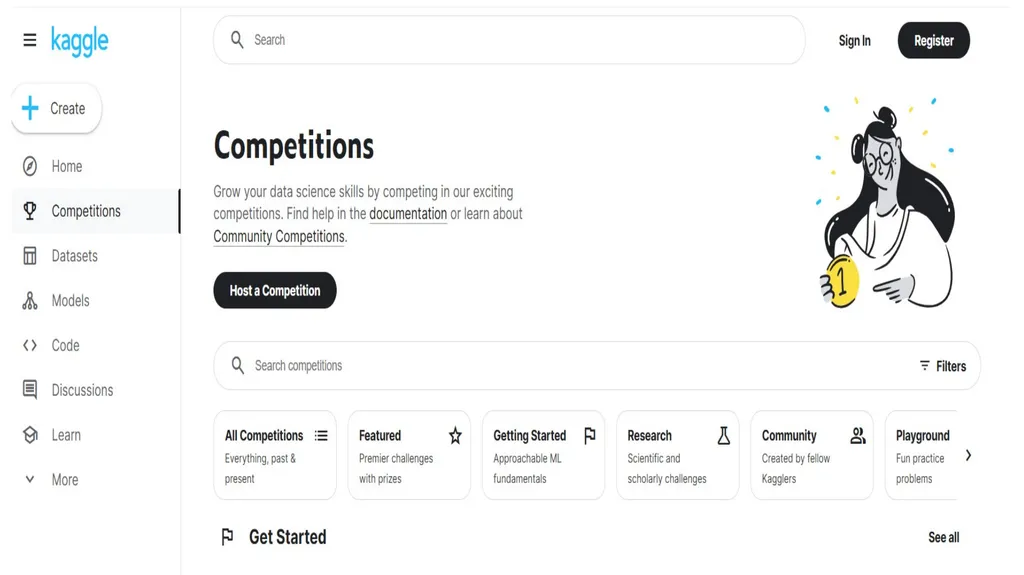
Kaggle Data Science Competition
https://www.kaggle.com/competitions What is Kaggle?
Kaggle is a platform for data science competitions.
Hosts challenges for data scientists and machine learning practitioners globally.
Provides a community for collaboration and learning.
Purpose of Competitions:
Solve real-world data problems.
Advance data science and machine learning fields.
Provide learning and networking opportunities.<br>
Kaggle is a platform for data science competitions.
Hosts challenges for data scientists and machine learning practitioners globally.
Provides a community for collaboration and learning.
Purpose of Competitions:
Solve real-world data problems.
Advance data science and machine learning fields.
Provide learning and networking opportunities.<br>
04
Structure and Types of Kaggle Competitions Competition Structure:
Problem Statement: Detailed description of the challenge.
Datasets: Training set (with targets) and test set (without targets).
Evaluation Metric: Criteria for judging model performance (e.g., accuracy, MSE).
Submissions: Multiple model submissions allowed.
Leaderboard: Ranks participants based on their scores.
Types of Competitions:
Featured Competitions: Sponsored by companies, with cash prizes.
Research Competitions: Focused on academic research.
Community Competitions: Created by the Kaggle community for learning.<br>
Problem Statement: Detailed description of the challenge.
Datasets: Training set (with targets) and test set (without targets).
Evaluation Metric: Criteria for judging model performance (e.g., accuracy, MSE).
Submissions: Multiple model submissions allowed.
Leaderboard: Ranks participants based on their scores.
Types of Competitions:
Featured Competitions: Sponsored by companies, with cash prizes.
Research Competitions: Focused on academic research.
Community Competitions: Created by the Kaggle community for learning.<br>
05
Benefits of Participating in Kaggle Competitions 1. Skill Development:
Hands-on experience with real-world data problems.
Learn data cleaning, feature engineering, and model evaluation.
2. Networking:
Connect with a global community of data scientists.
Collaborate and share insights on Kaggle forums.
3. Exposure:
Gain visibility in the data science community.
Attract job offers and consulting opportunities.
4. Crowdsourcing Solutions:
Companies can crowdsource innovative solutions.
Access diverse talent and ideas.<br>
Hands-on experience with real-world data problems.
Learn data cleaning, feature engineering, and model evaluation.
2. Networking:
Connect with a global community of data scientists.
Collaborate and share insights on Kaggle forums.
3. Exposure:
Gain visibility in the data science community.
Attract job offers and consulting opportunities.
4. Crowdsourcing Solutions:
Companies can crowdsource innovative solutions.
Access diverse talent and ideas.<br>
06
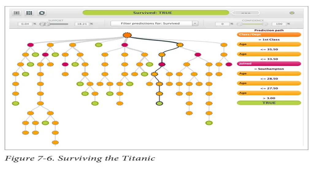
Example Competition: Titanic: Machine Learning from Disaster One of the most famous and beginner-friendly competitions on Kaggle is the "Titanic: Machine Learning from Disaster" competition. In this competition, participants are challenged to build a predictive model that determines whether a passenger on the Titanic survived or perished based on features such as age, gender, and class.
Training Data: Includes information about each passenger and whether they survived.
Test Data: Includes similar information but without the survival outcome, which participants must predict.
Evaluation Metric: Accuracy, which is the percentage of correct predictions out of the total predictions made.
This competition serves as an excellent starting point for those new to data science, allowing them to learn about data cleaning, feature engineering, and model evaluation in a hands-on way.<br>
Training Data: Includes information about each passenger and whether they survived.
Test Data: Includes similar information but without the survival outcome, which participants must predict.
Evaluation Metric: Accuracy, which is the percentage of correct predictions out of the total predictions made.
This competition serves as an excellent starting point for those new to data science, allowing them to learn about data cleaning, feature engineering, and model evaluation in a hands-on way.<br>
07
Titanic - Machine Learning from Disaster | Kaggle https://www.kaggle.com/competitions/titanic<br>
08
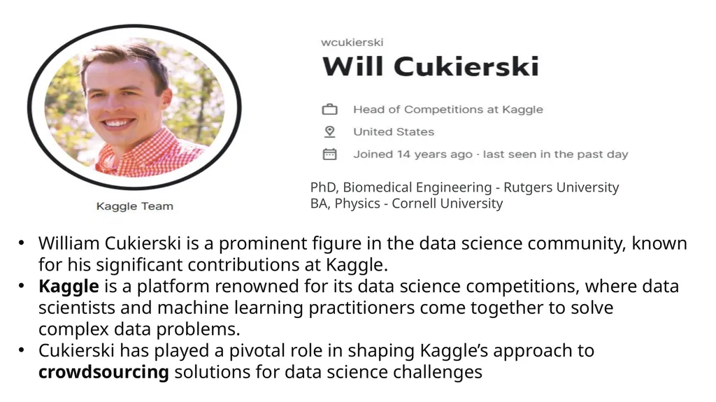
PhD, Biomedical Engineering - Rutgers University
BA, Physics - Cornell University William Cukierski is a prominent figure in the data science community, known for his significant contributions at Kaggle.
Kaggle is a platform renowned for its data science competitions, where data scientists and machine learning practitioners come together to solve complex data problems.
Cukierski has played a pivotal role in shaping Kaggle’s approach to crowdsourcing solutions for data science challenges<br>
Kaggle is a platform renowned for its data science competitions, where data scientists and machine learning practitioners come together to solve complex data problems.
Cukierski has played a pivotal role in shaping Kaggle’s approach to crowdsourcing solutions for data science challenges<br>
09
Background and Role: Cukierski holds a Ph.D. in biomedical engineering and has extensive experience in machine learning and data science.
At Kaggle, he has been instrumental in designing and managing competitions that help companies leverage the collective intelligence of the global data science community to tackle their toughest data challenges.<br>
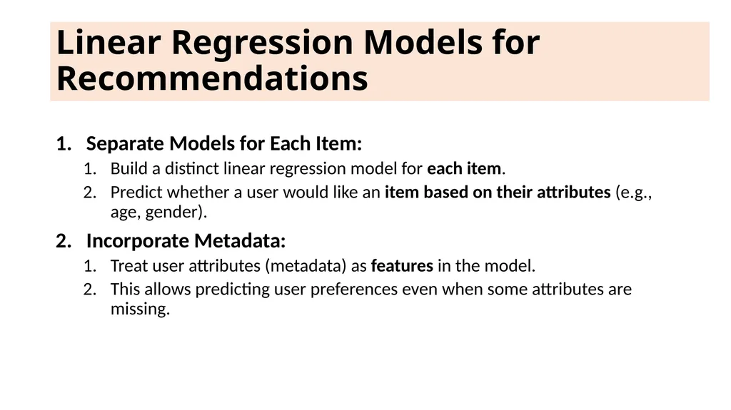
At Kaggle, he has been instrumental in designing and managing competitions that help companies leverage the collective intelligence of the global data science community to tackle their toughest data challenges.<br>
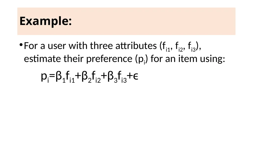
10
Contributions: His work involves ensuring that data problems are well-posed and that the competition structure allows for iterative improvement and innovation.
Through these competitions, Cukierski has helped foster a collaborative environment where data scientists can test their skills, share insights, and contribute to solving real-world problems.<br>
Through these competitions, Cukierski has helped foster a collaborative environment where data scientists can test their skills, share insights, and contribute to solving real-world problems.<br>
11
David Huffaker: David Huffaker is a distinguished researcher and data scientist at Google, specializing in social research and data analysis.
Google, as a tech giant, relies heavily on data-driven insights to refine its products and services, and Huffaker’s work is central to these efforts.<br>
Google, as a tech giant, relies heavily on data-driven insights to refine its products and services, and Huffaker’s work is central to these efforts.<br>
12
Background and Role: Huffaker has a background in communication and technology, with a focus on understanding user behavior and social interactions through data.
At Google, he combines qualitative and quantitative research methods to extract meaningful insights from data, helping to inform product development and user experience strategies.<br>
At Google, he combines qualitative and quantitative research methods to extract meaningful insights from data, helping to inform product development and user experience strategies.<br>
13
Contributions: Huffaker is known for his hybrid approach to data analysis, which integrates large-scale data analytics with qualitative insights.
This approach provides a more comprehensive understanding of user behavior, enabling Google to create products that better meet user needs and expectations.
He also emphasizes the importance of ethical considerations and privacy in data handling, ensuring that user data is used responsibly and transparently.<br>
This approach provides a more comprehensive understanding of user behavior, enabling Google to create products that better meet user needs and expectations.
He also emphasizes the importance of ethical considerations and privacy in data handling, ensuring that user data is used responsibly and transparently.<br>
14
Extracting Meaning from Data Extracting meaning from data involves interpreting raw data to gain insights, identify patterns, and make informed decisions.
This process is fundamental in data science and can be achieved through various methodologies, including statistical analysis, machine learning, and data visualization.<br>
This process is fundamental in data science and can be achieved through various methodologies, including statistical analysis, machine learning, and data visualization.<br>
15
Insights Insights are deep understandings derived from analyzing data, which can lead to actionable conclusions. These insights often reveal underlying trends, behaviors, or issues that were not immediately apparent.<br>
16
Example 1: Customer Behavior in Retail Data: Sales transactions, customer demographics, and purchase history.
Insight: Analysis reveals that customers aged 25-34 are significantly more likely to purchase eco-friendly products compared to other age groups.
Action: The retailer can increase marketing efforts and product offerings targeted at this demographic to boost sales of eco-friendly products.<br>
Insight: Analysis reveals that customers aged 25-34 are significantly more likely to purchase eco-friendly products compared to other age groups.
Action: The retailer can increase marketing efforts and product offerings targeted at this demographic to boost sales of eco-friendly products.<br>
17
Example 2: Website Performance Data: Web traffic, user engagement metrics, and conversion rates.
Insight: A high bounce rate on a specific landing page suggests that visitors are not finding what they expect.
Action: Revise the content and layout of the landing page to better align with user expectations and improve engagement.<br>
Insight: A high bounce rate on a specific landing page suggests that visitors are not finding what they expect.
Action: Revise the content and layout of the landing page to better align with user expectations and improve engagement.<br>
18
Patterns Patterns are recurring themes or structures in data that can be identified through statistical analysis or data mining techniques.
Recognizing patterns can help in predicting future events or behaviors.<br>
Recognizing patterns can help in predicting future events or behaviors.<br>
19
Example 1: Seasonal Sales Patterns Data: Monthly sales data over several years.
Pattern: There is a consistent spike in sales every December, followed by a dip in January.
Action: Prepare for increased inventory and marketing campaigns in November and December to capitalize on the holiday season, and plan promotions or discounts to boost sales in January.<br>
Pattern: There is a consistent spike in sales every December, followed by a dip in January.
Action: Prepare for increased inventory and marketing campaigns in November and December to capitalize on the holiday season, and plan promotions or discounts to boost sales in January.<br>
20
Example 2: Customer Churn in Subscription Services Data: User activity logs, subscription renewal rates, and customer service interactions.
Pattern: Customers who have not used the service in the last two weeks and have contacted customer service with complaints are more likely to churn.
Action: Implement a proactive outreach program to re-engage these at-risk customers and address their issues before they decide to cancel their subscriptions.<br>
Pattern: Customers who have not used the service in the last two weeks and have contacted customer service with complaints are more likely to churn.
Action: Implement a proactive outreach program to re-engage these at-risk customers and address their issues before they decide to cancel their subscriptions.<br>
21
Combining Insights and Patterns Combining insights and patterns can provide a more comprehensive understanding of data, leading to more effective strategies and decisions.<br>
22
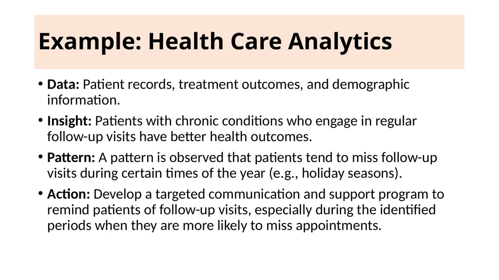
Example: Health Care Analytics Data: Patient records, treatment outcomes, and demographic information.
Insight: Patients with chronic conditions who engage in regular follow-up visits have better health outcomes.
Pattern: A pattern is observed that patients tend to miss follow-up visits during certain times of the year (e.g., holiday seasons).
Action: Develop a targeted communication and support program to remind patients of follow-up visits, especially during the identified periods when they are more likely to miss appointments.<br>
Insight: Patients with chronic conditions who engage in regular follow-up visits have better health outcomes.
Pattern: A pattern is observed that patients tend to miss follow-up visits during certain times of the year (e.g., holiday seasons).
Action: Develop a targeted communication and support program to remind patients of follow-up visits, especially during the identified periods when they are more likely to miss appointments.<br>
23
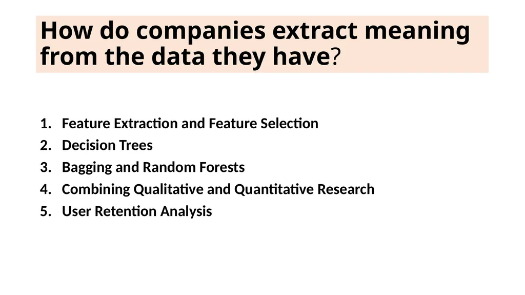
How do companies extract meaning from the data they have? Feature Extraction and Feature Selection
Decision Trees
Bagging and Random Forests
Combining Qualitative and Quantitative Research
User Retention Analysis<br>
Decision Trees
Bagging and Random Forests
Combining Qualitative and Quantitative Research
User Retention Analysis<br>
24
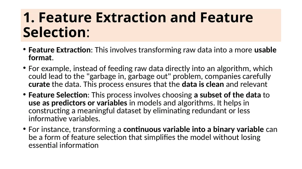
1. Feature Extraction and Feature Selection: Feature Extraction: This involves transforming raw data into a more usable format.
For example, instead of feeding raw data directly into an algorithm, which could lead to the "garbage in, garbage out" problem, companies carefully curate the data. This process ensures that the data is clean and relevant
Feature Selection: This process involves choosing a subset of the data to use as predictors or variables in models and algorithms. It helps in constructing a meaningful dataset by eliminating redundant or less informative variables.
For instance, transforming a continuous variable into a binary variable can be a form of feature selection that simplifies the model without losing essential information<br>
For example, instead of feeding raw data directly into an algorithm, which could lead to the "garbage in, garbage out" problem, companies carefully curate the data. This process ensures that the data is clean and relevant
Feature Selection: This process involves choosing a subset of the data to use as predictors or variables in models and algorithms. It helps in constructing a meaningful dataset by eliminating redundant or less informative variables.
For instance, transforming a continuous variable into a binary variable can be a form of feature selection that simplifies the model without losing essential information<br>
25
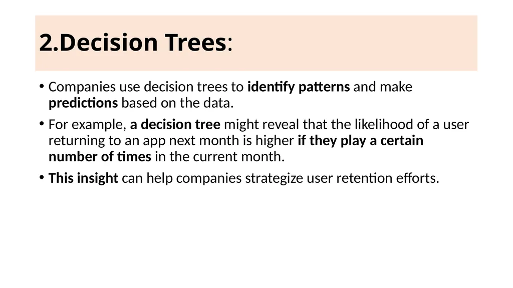
2.Decision Trees: Companies use decision trees to identify patterns and make predictions based on the data.
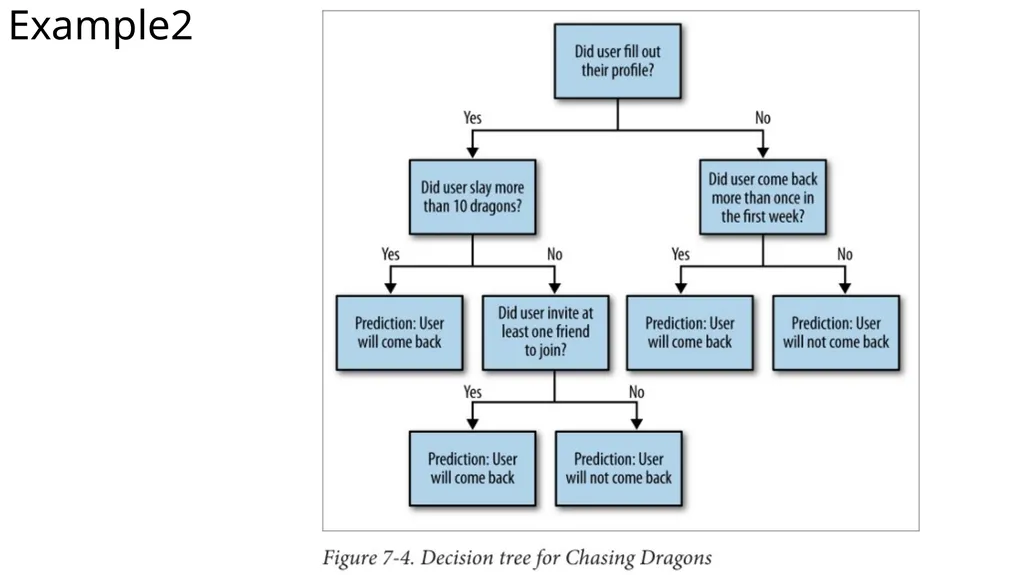
For example, a decision tree might reveal that the likelihood of a user returning to an app next month is higher if they play a certain number of times in the current month.
This insight can help companies strategize user retention efforts.<br>
For example, a decision tree might reveal that the likelihood of a user returning to an app next month is higher if they play a certain number of times in the current month.
This insight can help companies strategize user retention efforts.<br>
26
3.Bagging and Random Forests Bagging, or bootstrap aggregating, helps in reducing variance in predictions by averaging the results of multiple models.
Random forests, which are an extension of bagging, further enhance this by incorporating multiple decision trees to improve predictive accuracy and handle idiosyncratic noise in the data<br>
Random forests, which are an extension of bagging, further enhance this by incorporating multiple decision trees to improve predictive accuracy and handle idiosyncratic noise in the data<br>
27
4.Combining Qualitative and Quantitative Research: A hybrid approach that combines both qualitative insights and quantitative data helps in deriving more nuanced understandings.
For instance, qualitative research might identify user behavior patterns on a small scale, which can then be validated and expanded using large-scale quantitative data.
This approach ensures that the insights are both statistically significant and contextually rich.<br>
For instance, qualitative research might identify user behavior patterns on a small scale, which can then be validated and expanded using large-scale quantitative data.
This approach ensures that the insights are both statistically significant and contextually rich.<br>
28
5.User Retention Analysis By building models that predict user behavior, such as whether a user will continue using an app, companies can tailor their strategies to enhance user retention.
For example, a model might suggest that showing ads within the first five minutes decreases retention rates, guiding companies to adjust their advertising strategies accordingly.<br>
For example, a model might suggest that showing ads within the first five minutes decreases retention rates, guiding companies to adjust their advertising strategies accordingly.<br>
29
Perspectives of William Cukierski from Kaggle and David Huffaker from Google From the perspectives of William Cukierski from Kaggle and David Huffaker from Google, companies extract meaning from the data they have through distinct methodologies and approaches<br>
30
William Cukierski's Perspective (Kaggle) William Cukierski emphasizes the importance of feature extraction and feature selection in data science. He outlines the following processes:
Feature Extraction: Transforming raw data into a curated format to avoid the "garbage in, garbage out" problem. This process ensures that the data fed into algorithms is clean and relevant.
Feature Selection: Constructing a subset of data or functions of data to be predictors or variables for models and algorithms. This helps in reducing redundancy and focusing on the most informative variables.
Kaggle Competitions: Kaggle hosts competitions that crowdsource solutions from data scientists worldwide. Participants are given training sets and test sets where they apply their models to make predictions. The competitions foster a "leapfrogging" effect, encouraging iterative improvement and innovation in model building.
Crowdsourcing: Leveraging the collective intelligence of the global data science community to solve complex data problems for businesses. This approach allows companies to tap into a diverse pool of talent and ideas, leading to more robust and creative solutions.<br>
Feature Extraction: Transforming raw data into a curated format to avoid the "garbage in, garbage out" problem. This process ensures that the data fed into algorithms is clean and relevant.
Feature Selection: Constructing a subset of data or functions of data to be predictors or variables for models and algorithms. This helps in reducing redundancy and focusing on the most informative variables.
Kaggle Competitions: Kaggle hosts competitions that crowdsource solutions from data scientists worldwide. Participants are given training sets and test sets where they apply their models to make predictions. The competitions foster a "leapfrogging" effect, encouraging iterative improvement and innovation in model building.
Crowdsourcing: Leveraging the collective intelligence of the global data science community to solve complex data problems for businesses. This approach allows companies to tap into a diverse pool of talent and ideas, leading to more robust and creative solutions.<br>
31
David Huffaker's Perspective (Google) David Huffaker from Google takes a hybrid approach to social research, combining qualitative insights with quantitative data. His key points include:
Descriptive to Predictive Analysis: Moving from simply describing data to predicting future trends and behaviors. This involves building models that can forecast outcomes based on historical data.
Combining Qualitative and Quantitative Research: Integrating qualitative research, such as user interviews and ethnographic studies, with large-scale quantitative data analysis. This hybrid approach provides a more comprehensive understanding of user behavior and social trends.
User Retention Models: Developing models that predict user retention based on various factors, such as user activity and engagement patterns. These models help in strategizing to improve user retention and satisfaction
Ethical Considerations: Addressing privacy concerns and ensuring ethical use of data. Huffaker emphasizes the importance of transparency and user control over their data to build trust and mitigate privacy risks.<br>
Descriptive to Predictive Analysis: Moving from simply describing data to predicting future trends and behaviors. This involves building models that can forecast outcomes based on historical data.
Combining Qualitative and Quantitative Research: Integrating qualitative research, such as user interviews and ethnographic studies, with large-scale quantitative data analysis. This hybrid approach provides a more comprehensive understanding of user behavior and social trends.
User Retention Models: Developing models that predict user retention based on various factors, such as user activity and engagement patterns. These models help in strategizing to improve user retention and satisfaction
Ethical Considerations: Addressing privacy concerns and ensuring ethical use of data. Huffaker emphasizes the importance of transparency and user control over their data to build trust and mitigate privacy risks.<br>
32
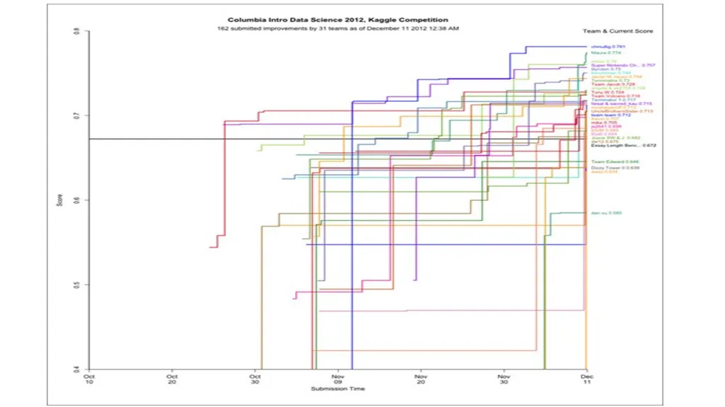
Kaggle Model Competition
Leapfrogging (Economic/Technological/Innovation) Visualization
Score Tracking
Submission Timeline
Team Identification
Encouraging Partition
Kaggle Customers<br>
Leapfrogging (Economic/Technological/Innovation) Visualization
Score Tracking
Submission Timeline
Team Identification
Encouraging Partition
Kaggle Customers<br>
33
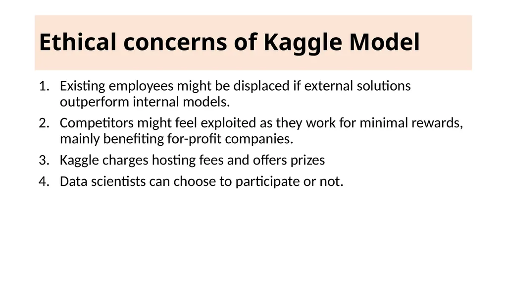
Ethical concerns of Kaggle Model Existing employees might be displaced if external solutions outperform internal models.
Competitors might feel exploited as they work for minimal rewards, mainly benefiting for-profit companies.
Kaggle charges hosting fees and offers prizes
Data scientists can choose to participate or not.<br>
Competitors might feel exploited as they work for minimal rewards, mainly benefiting for-profit companies.
Kaggle charges hosting fees and offers prizes
Data scientists can choose to participate or not.<br>
34
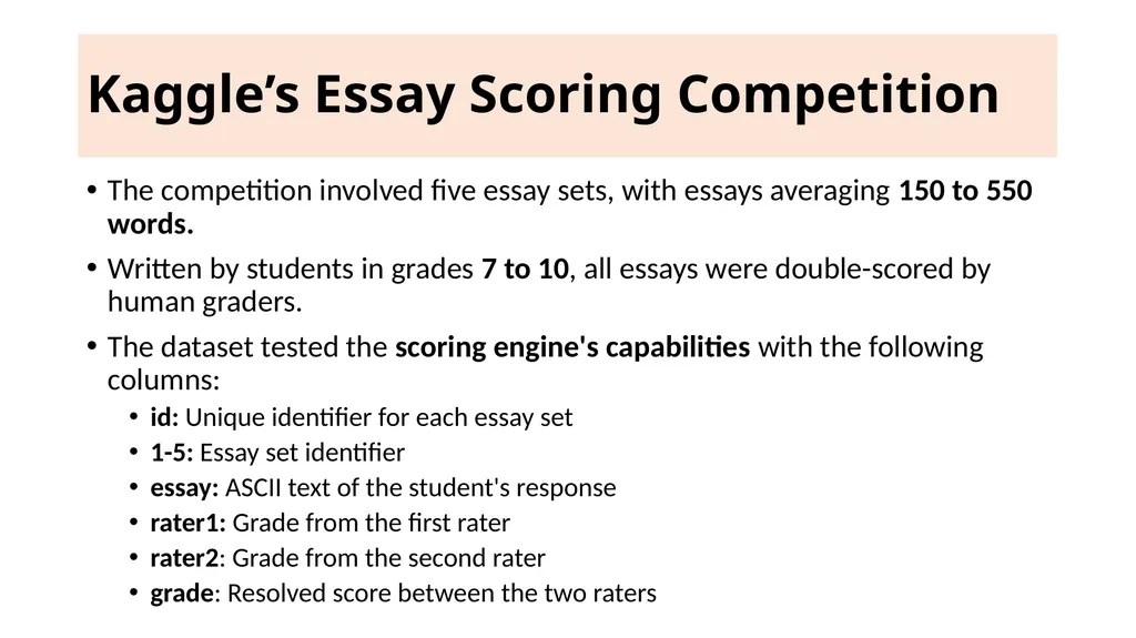
Kaggle’s Essay Scoring Competition The competition involved five essay sets, with essays averaging 150 to 550 words.
Written by students in grades 7 to 10, all essays were double-scored by human graders.
The dataset tested the scoring engine's capabilities with the following columns:
id: Unique identifier for each essay set
1-5: Essay set identifier
essay: ASCII text of the student's response
rater1: Grade from the first rater
rater2: Grade from the second rater
grade: Resolved score between the two raters<br>
Written by students in grades 7 to 10, all essays were double-scored by human graders.
The dataset tested the scoring engine's capabilities with the following columns:
id: Unique identifier for each essay set
1-5: Essay set identifier
essay: ASCII text of the student's response
rater1: Grade from the first rater
rater2: Grade from the second rater
grade: Resolved score between the two raters<br>
35
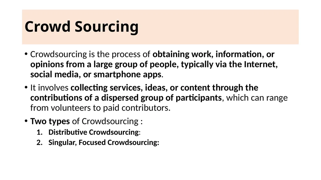
Crowd Sourcing Crowdsourcing is the process of obtaining work, information, or opinions from a large group of people, typically via the Internet, social media, or smartphone apps.
It involves collecting services, ideas, or content through the contributions of a dispersed group of participants, which can range from volunteers to paid contributors.
Two types of Crowdsourcing :
Distributive Crowdsourcing:
Singular, Focused Crowdsourcing:<br>
It involves collecting services, ideas, or content through the contributions of a dispersed group of participants, which can range from volunteers to paid contributors.
Two types of Crowdsourcing :
Distributive Crowdsourcing:
Singular, Focused Crowdsourcing:<br>
36
1.Distributive Crowdsourcing Example: Wikipedia.
Involves large-scale, simplistic contributions.
Open to anyone to contribute with volunteer-based regulation and quality control.<br>
Involves large-scale, simplistic contributions.
Open to anyone to contribute with volunteer-based regulation and quality control.<br>
37
2. Singular, Focused Crowdsourcing: Examples: Kaggle, DARPA, InnoCentive.
Involves solving complex problems by skilled individuals.
Offers cash prizes and community recognition.<br>
Involves solving complex problems by skilled individuals.
Offers cash prizes and community recognition.<br>
38
Domain Expertise Versus Machine Learning Algorithms Both are needed to solve data science problems:
Information Quality
Algorithmic Advantage
Role of Experts
Black Box Approach<br>
Information Quality
Algorithmic Advantage
Role of Experts
Black Box Approach<br>
39
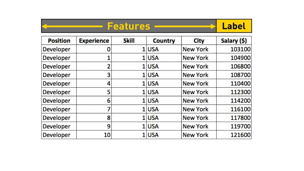
What are Features in Data Set? Features in a dataset are individual measurable properties or characteristics of a phenomenon being observed.
Each feature corresponds to a column in a data set, where each row represents an observation or record
In the context of machine learning and data science, features are used as input variables to models.
They represent the data points that help in predicting outcomes or understanding patterns within the dataset.
Examples: Common examples include variables like height, weight, temperature, and volume<br>
Each feature corresponds to a column in a data set, where each row represents an observation or record
In the context of machine learning and data science, features are used as input variables to models.
They represent the data points that help in predicting outcomes or understanding patterns within the dataset.
Examples: Common examples include variables like height, weight, temperature, and volume<br>
40
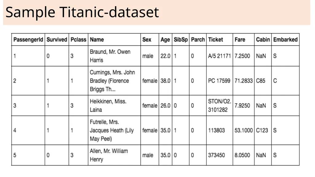
Sample Titanic-dataset<br>
41
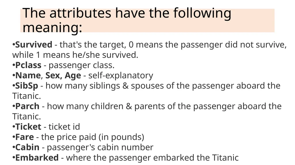
The attributes have the following meaning: Survived - that's the target, 0 means the passenger did not survive, while 1 means he/she survived.
Pclass - passenger class.
Name, Sex, Age - self-explanatory
SibSp - how many siblings & spouses of the passenger aboard the Titanic.
Parch - how many children & parents of the passenger aboard the Titanic.
Ticket - ticket id
Fare - the price paid (in pounds)
Cabin - passenger's cabin number
Embarked - where the passenger embarked the Titanic<br>
Pclass - passenger class.
Name, Sex, Age - self-explanatory
SibSp - how many siblings & spouses of the passenger aboard the Titanic.
Parch - how many children & parents of the passenger aboard the Titanic.
Ticket - ticket id
Fare - the price paid (in pounds)
Cabin - passenger's cabin number
Embarked - where the passenger embarked the Titanic<br>
42
You can ignore name, id and ticket# columns because these are just identifiers and don't offer value as a feature.<br>
43
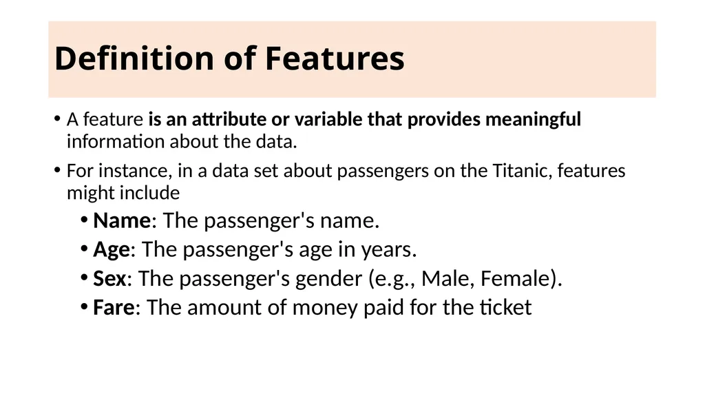
Definition of Features A feature is an attribute or variable that provides meaningful information about the data.
For instance, in a data set about passengers on the Titanic, features might include
Name: The passenger's name.
Age: The passenger's age in years.
Sex: The passenger's gender (e.g., Male, Female).
Fare: The amount of money paid for the ticket<br>
For instance, in a data set about passengers on the Titanic, features might include
Name: The passenger's name.
Age: The passenger's age in years.
Sex: The passenger's gender (e.g., Male, Female).
Fare: The amount of money paid for the ticket<br>
44
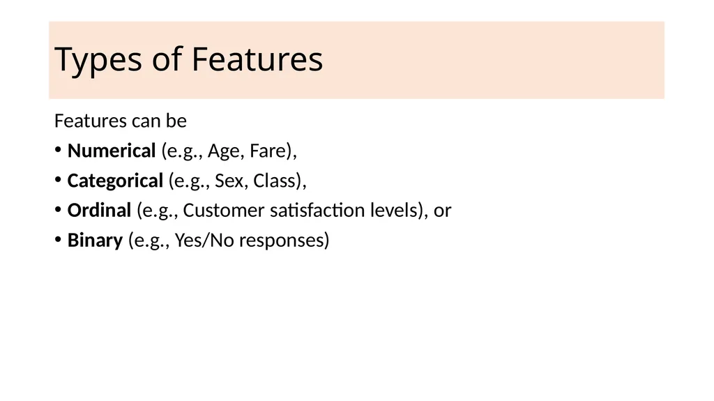
Types of Features Features can be
Numerical (e.g., Age, Fare),
Categorical (e.g., Sex, Class),
Ordinal (e.g., Customer satisfaction levels), or
Binary (e.g., Yes/No responses)<br>
Numerical (e.g., Age, Fare),
Categorical (e.g., Sex, Class),
Ordinal (e.g., Customer satisfaction levels), or
Binary (e.g., Yes/No responses)<br>
45
Importance of Features in Data Sets Identifying and understanding the right features in a data set is crucial for effective data analysis and achieving accurate results in predictive modeling.<br>
46
Feature Selection Feature selection is a crucial step in the process of building effective predictive models in data science and machine learning.
It involves identifying and selecting a subset of relevant features (or variables) from the total available data to be used in model building.<br>
It involves identifying and selecting a subset of relevant features (or variables) from the total available data to be used in model building.<br>
47
Why Feature Selection is Important Reducing Overfitting: By removing irrelevant or redundant features, the model becomes less complex and generalizes better to new data.
Improving Performance: Fewer features mean less computational power is required, leading to faster model training and prediction.
Enhanced Interpretability: Models with fewer features are easier to understand and interpret.<br>
Improving Performance: Fewer features mean less computational power is required, leading to faster model training and prediction.
Enhanced Interpretability: Models with fewer features are easier to understand and interpret.<br>
48
Techniques for Feature Selection Filters
Wrappers
Embedded
Hybrid<br>
Wrappers
Embedded
Hybrid<br>
49
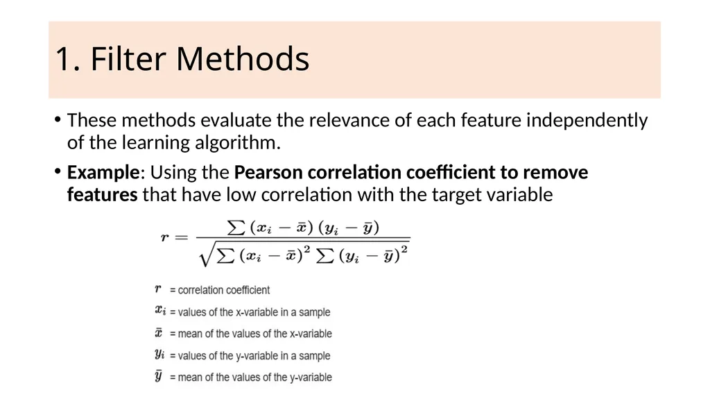
1. Filter Methods These methods evaluate the relevance of each feature independently of the learning algorithm.
Example: Using the Pearson correlation coefficient to remove features that have low correlation with the target variable<br>
Example: Using the Pearson correlation coefficient to remove features that have low correlation with the target variable<br>
50
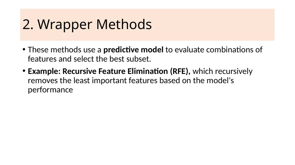
2. Wrapper Methods These methods use a predictive model to evaluate combinations of features and select the best subset.
Example: Recursive Feature Elimination (RFE), which recursively removes the least important features based on the model's performance<br>
Example: Recursive Feature Elimination (RFE), which recursively removes the least important features based on the model's performance<br>
51
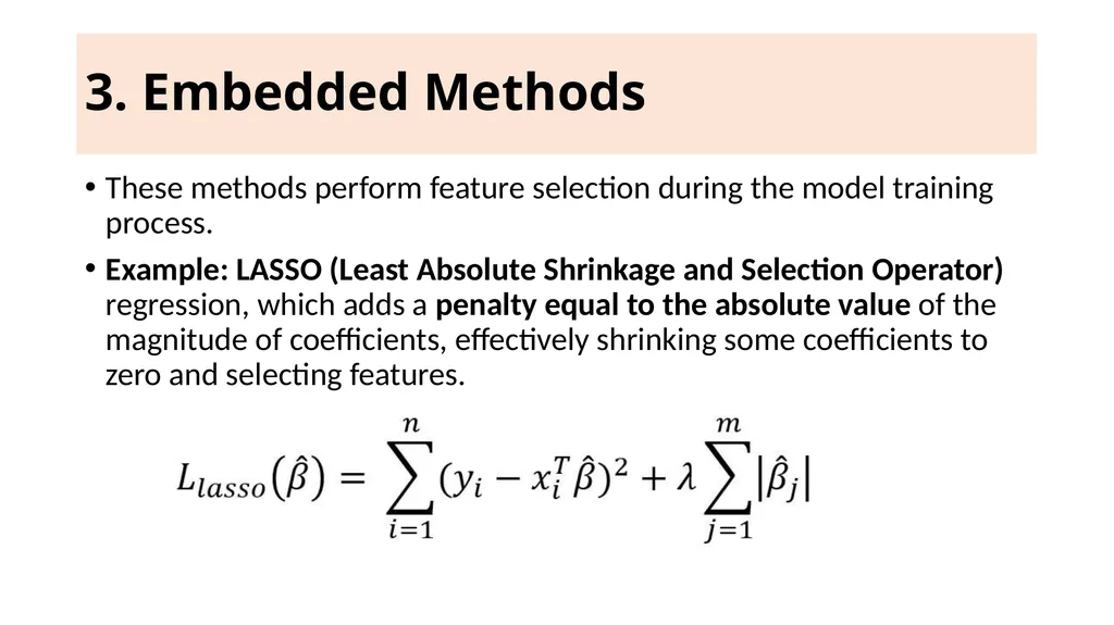
3. Embedded Methods These methods perform feature selection during the model training process.
Example: LASSO (Least Absolute Shrinkage and Selection Operator) regression, which adds a penalty equal to the absolute value of the magnitude of coefficients, effectively shrinking some coefficients to zero and selecting features.<br>
Example: LASSO (Least Absolute Shrinkage and Selection Operator) regression, which adds a penalty equal to the absolute value of the magnitude of coefficients, effectively shrinking some coefficients to zero and selecting features.<br>
52
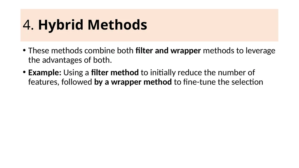
4. Hybrid Methods These methods combine both filter and wrapper methods to leverage the advantages of both.
Example: Using a filter method to initially reduce the number of features, followed by a wrapper method to fine-tune the selection<br>
Example: Using a filter method to initially reduce the number of features, followed by a wrapper method to fine-tune the selection<br>
53
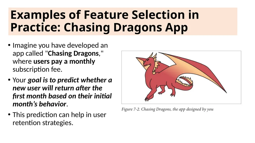
Examples of Feature Selection in Practice: Chasing Dragons App Imagine you have developed an app called "Chasing Dragons," where users pay a monthly subscription fee.
Your goal is to predict whether a new user will return after the first month based on their initial month’s behavior.
This prediction can help in user retention strategies.<br>
Your goal is to predict whether a new user will return after the first month based on their initial month’s behavior.
This prediction can help in user retention strategies.<br>
54
Here’s how you might approach feature selection for this problem Data Collection: Record every user action with timestamps during their first 30 days.
Feature Generation: Brainstorm possible features that might influence user retention.<br>
Feature Generation: Brainstorm possible features that might influence user retention.<br>
55
Example Features: Number of days the user visited in the first month.
Time until the second visit.
Points scored each day (30 separate features).
Total points in the first month.
Whether the user filled out their profile (binary feature).
User demographics such as age and gender.
Device characteristics like screen size.
Use your imagination and come up with as many features as possible. Notice there are redundancies and correlations between these features; that’s OK.<br>
Time until the second visit.
Points scored each day (30 separate features).
Total points in the first month.
Whether the user filled out their profile (binary feature).
User demographics such as age and gender.
Device characteristics like screen size.
Use your imagination and come up with as many features as possible. Notice there are redundancies and correlations between these features; that’s OK.<br>
56
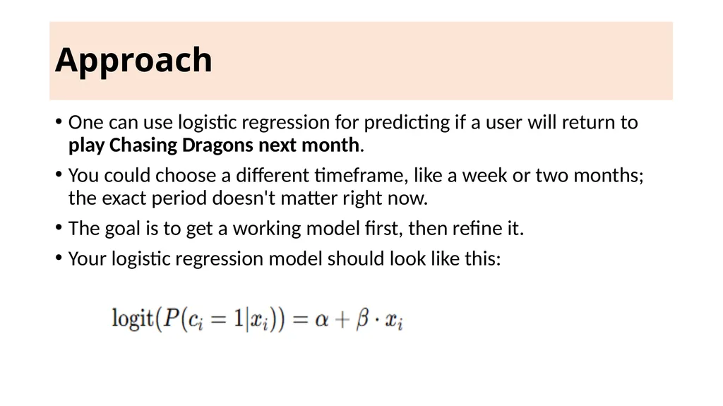
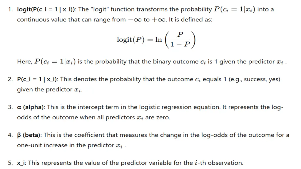
Approach One can use logistic regression for predicting if a user will return to play Chasing Dragons next month.
You could choose a different timeframe, like a week or two months; the exact period doesn't matter right now.
The goal is to get a working model first, then refine it.
Your logistic regression model should look like this:<br>
You could choose a different timeframe, like a week or two months; the exact period doesn't matter right now.
The goal is to get a working model first, then refine it.
Your logistic regression model should look like this:<br>
57
Feature Selection Methods: Filters: Use statistical methods to assess the relevance of each feature independently of the model. For example, you might use correlation coefficients to identify highly correlated features.
Wrappers: Evaluate subsets of features by training models and selecting the subset that performs best according to a chosen metric (e.g., accuracy, AUC).
Embedded Methods: Perform feature selection as part of the model training process. For example, regularization methods like Lasso (L1 regularization) can shrink some feature coefficients to zero, effectively performing feature selection.<br>
Wrappers: Evaluate subsets of features by training models and selecting the subset that performs best according to a chosen metric (e.g., accuracy, AUC).
Embedded Methods: Perform feature selection as part of the model training process. For example, regularization methods like Lasso (L1 regularization) can shrink some feature coefficients to zero, effectively performing feature selection.<br>
58
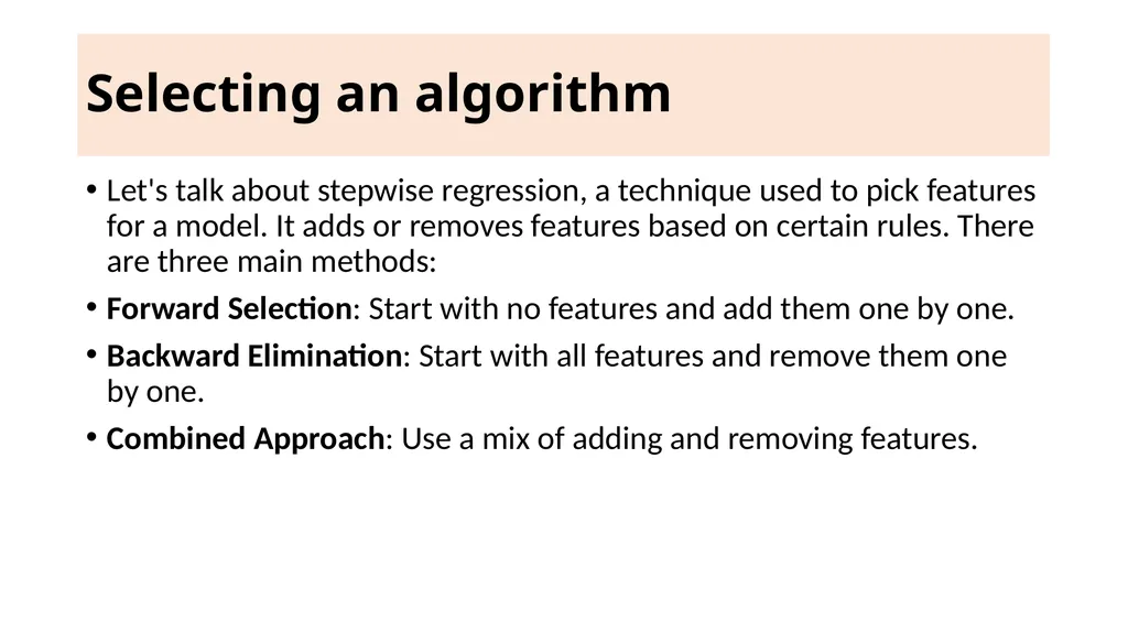
Selecting an algorithm Let's talk about stepwise regression, a technique used to pick features for a model. It adds or removes features based on certain rules. There are three main methods:
Forward Selection: Start with no features and add them one by one.
Backward Elimination: Start with all features and remove them one by one.
Combined Approach: Use a mix of adding and removing features.<br>
Forward Selection: Start with no features and add them one by one.
Backward Elimination: Start with all features and remove them one by one.
Combined Approach: Use a mix of adding and removing features.<br>
59
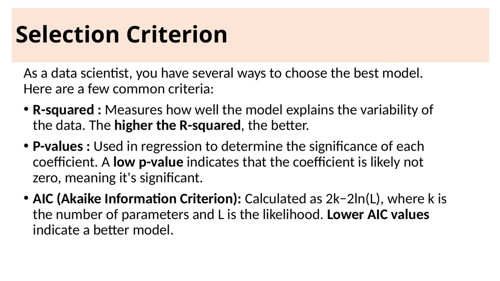
Selection Criterion As a data scientist, you have several ways to choose the best model. Here are a few common criteria:
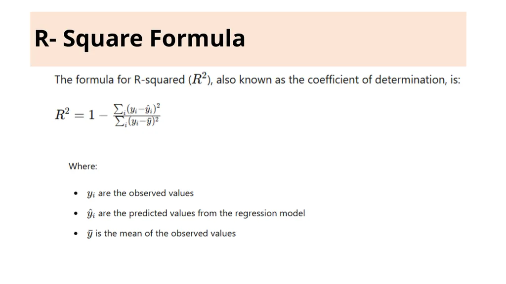
R-squared : Measures how well the model explains the variability of the data. The higher the R-squared, the better.
P-values : Used in regression to determine the significance of each coefficient. A low p-value indicates that the coefficient is likely not zero, meaning it's significant.
AIC (Akaike Information Criterion): Calculated as 2k−2ln(L), where k is the number of parameters and L is the likelihood. Lower AIC values indicate a better model.<br>
R-squared : Measures how well the model explains the variability of the data. The higher the R-squared, the better.
P-values : Used in regression to determine the significance of each coefficient. A low p-value indicates that the coefficient is likely not zero, meaning it's significant.
AIC (Akaike Information Criterion): Calculated as 2k−2ln(L), where k is the number of parameters and L is the likelihood. Lower AIC values indicate a better model.<br>
60
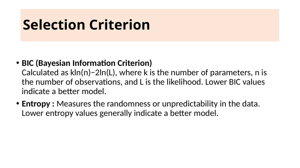
Selection Criterion BIC (Bayesian Information Criterion)
Calculated as kln(n)−2ln(L), where k is the number of parameters, n is the number of observations, and L is the likelihood. Lower BIC values indicate a better model.
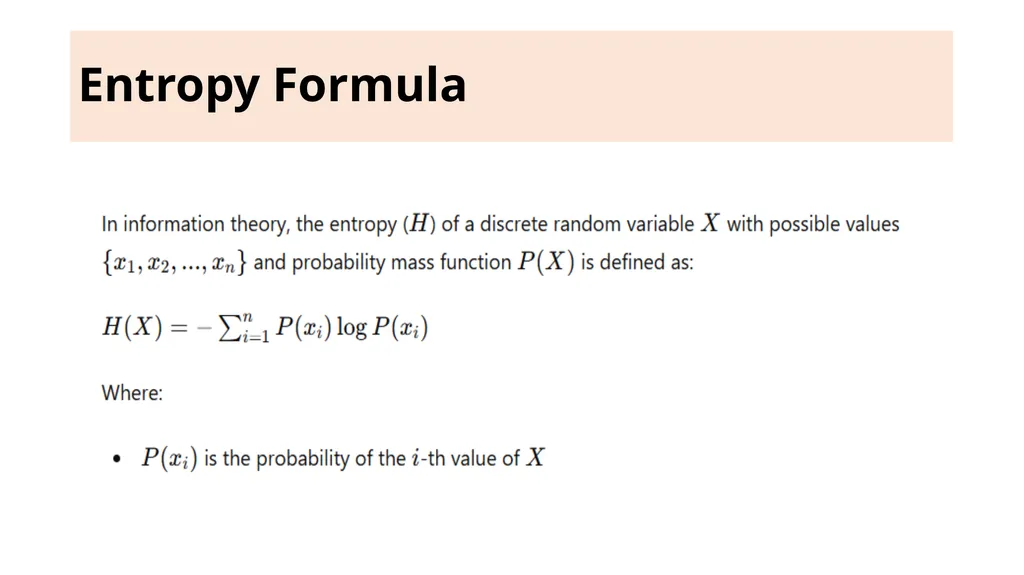
Entropy : Measures the randomness or unpredictability in the data. Lower entropy values generally indicate a better model.<br>
Entropy : Measures the randomness or unpredictability in the data. Lower entropy values generally indicate a better model.<br>
61
R- Square Formula<br>
62
Entropy Formula<br>
63
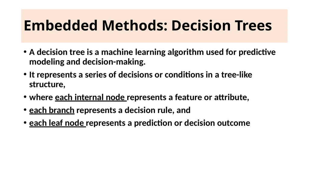
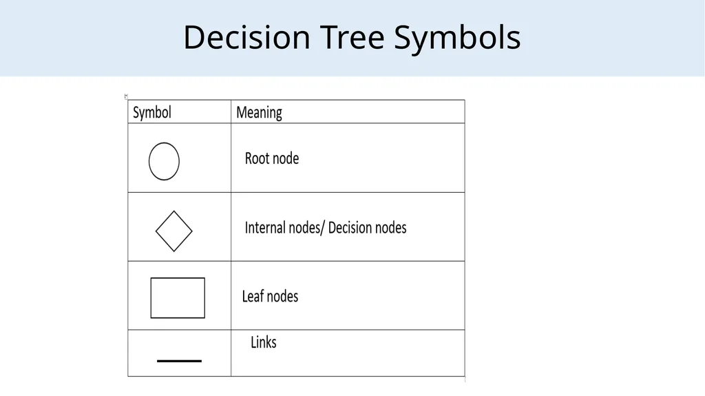
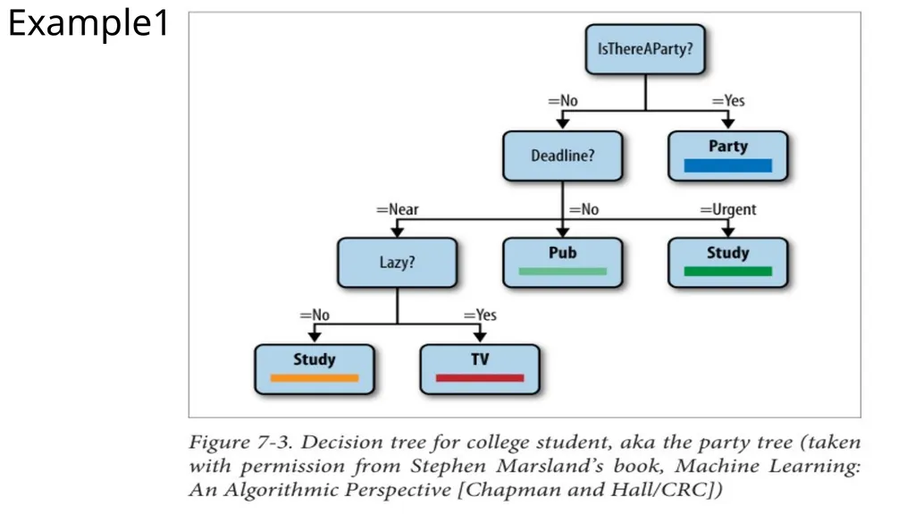
Embedded Methods: Decision Trees A decision tree is a machine learning algorithm used for predictive modeling and decision-making.
It represents a series of decisions or conditions in a tree-like structure,
where each internal node represents a feature or attribute,
each branch represents a decision rule, and
each leaf node represents a prediction or decision outcome<br>
It represents a series of decisions or conditions in a tree-like structure,
where each internal node represents a feature or attribute,
each branch represents a decision rule, and
each leaf node represents a prediction or decision outcome<br>
64
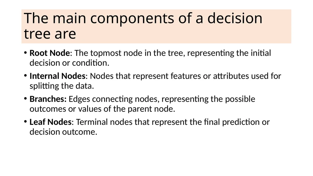
The main components of a decision tree are Root Node: The topmost node in the tree, representing the initial decision or condition.
Internal Nodes: Nodes that represent features or attributes used for splitting the data.
Branches: Edges connecting nodes, representing the possible outcomes or values of the parent node.
Leaf Nodes: Terminal nodes that represent the final prediction or decision outcome.<br>
Internal Nodes: Nodes that represent features or attributes used for splitting the data.
Branches: Edges connecting nodes, representing the possible outcomes or values of the parent node.
Leaf Nodes: Terminal nodes that represent the final prediction or decision outcome.<br>
65
Decision Tree Symbols<br>
66
Example1<br>
67
Example2<br>
68
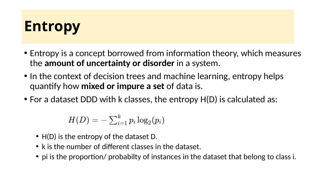
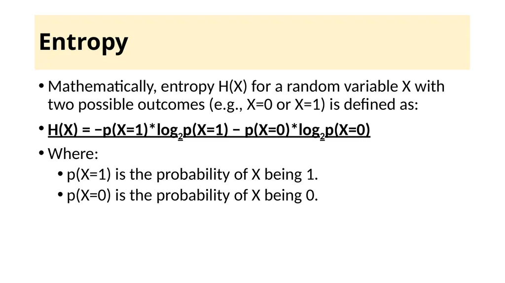
Entropy Entropy is a concept borrowed from information theory, which measures the amount of uncertainty or disorder in a system.
In the context of decision trees and machine learning, entropy helps quantify how mixed or impure a set of data is.
For a dataset DDD with k classes, the entropy H(D) is calculated as:
H(D) is the entropy of the dataset D.
k is the number of different classes in the dataset.
pi is the proportion/ probabilty of instances in the dataset that belong to class i.<br>
In the context of decision trees and machine learning, entropy helps quantify how mixed or impure a set of data is.
For a dataset DDD with k classes, the entropy H(D) is calculated as:
H(D) is the entropy of the dataset D.
k is the number of different classes in the dataset.
pi is the proportion/ probabilty of instances in the dataset that belong to class i.<br>
69
Entropy Mathematically, entropy H(X) for a random variable X with two possible outcomes (e.g., X=0 or X=1) is defined as:
H(X) = −p(X=1)*log2p(X=1) − p(X=0)*log2p(X=0)
Where:
p(X=1) is the probability of X being 1.
p(X=0) is the probability of X being 0.<br>
H(X) = −p(X=1)*log2p(X=1) − p(X=0)*log2p(X=0)
Where:
p(X=1) is the probability of X being 1.
p(X=0) is the probability of X being 0.<br>
70
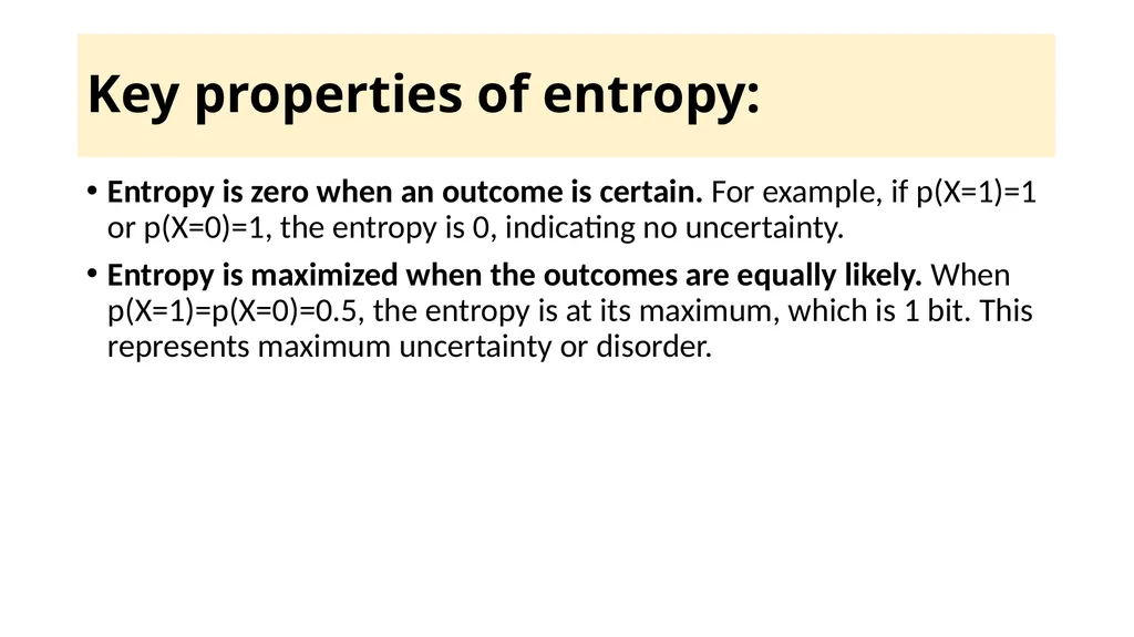
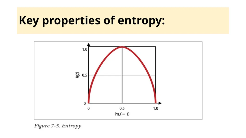
Key properties of entropy: Entropy is zero when an outcome is certain. For example, if p(X=1)=1 or p(X=0)=1, the entropy is 0, indicating no uncertainty.
Entropy is maximized when the outcomes are equally likely. When p(X=1)=p(X=0)=0.5, the entropy is at its maximum, which is 1 bit. This represents maximum uncertainty or disorder.<br>
Entropy is maximized when the outcomes are equally likely. When p(X=1)=p(X=0)=0.5, the entropy is at its maximum, which is 1 bit. This represents maximum uncertainty or disorder.<br>
71
Key properties of entropy:<br>
72
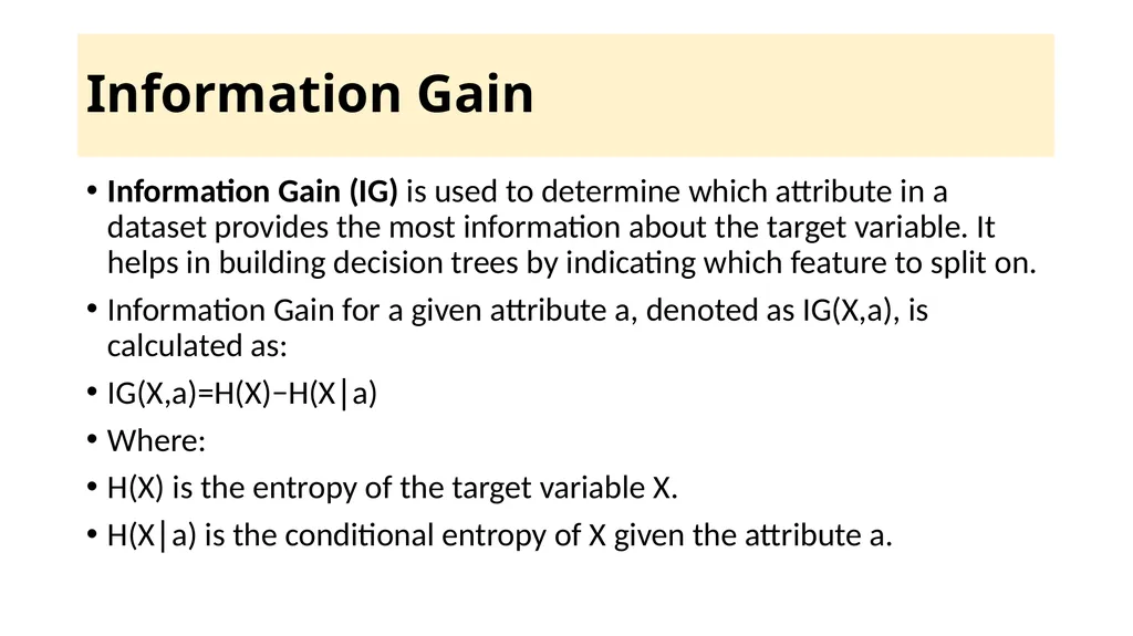
Information Gain Information Gain (IG) is used to determine which attribute in a dataset provides the most information about the target variable. It helps in building decision trees by indicating which feature to split on.
Information Gain for a given attribute a, denoted as IG(X,a), is calculated as:
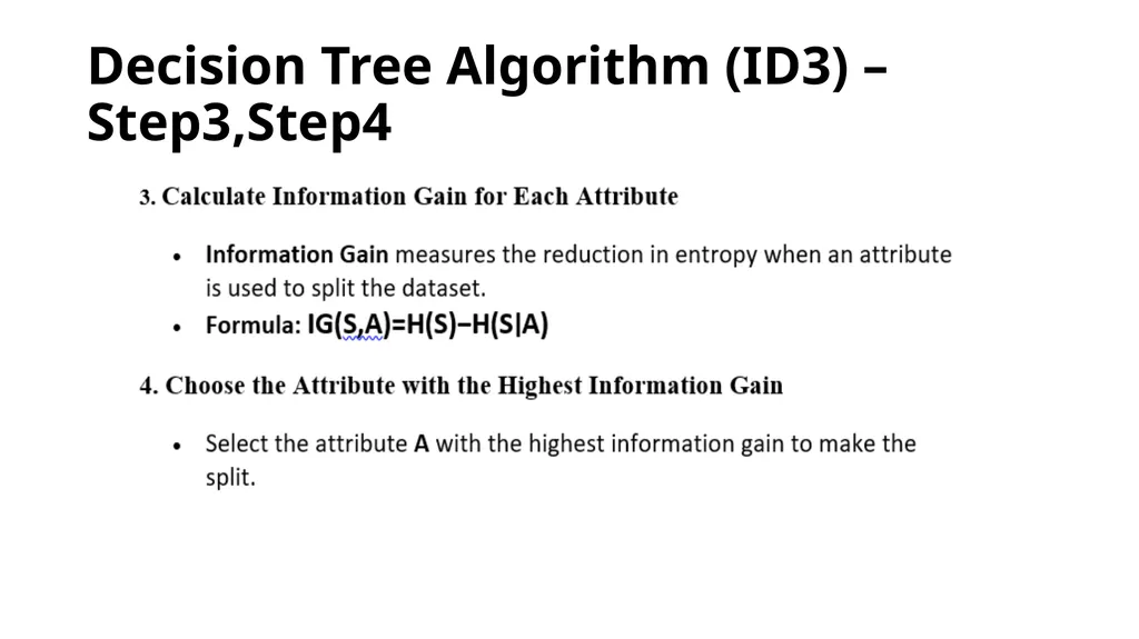
IG(X,a)=H(X)−H(X∣a)
Where:
H(X) is the entropy of the target variable X.
H(X∣a) is the conditional entropy of X given the attribute a.<br>
Information Gain for a given attribute a, denoted as IG(X,a), is calculated as:
IG(X,a)=H(X)−H(X∣a)
Where:
H(X) is the entropy of the target variable X.
H(X∣a) is the conditional entropy of X given the attribute a.<br>
73
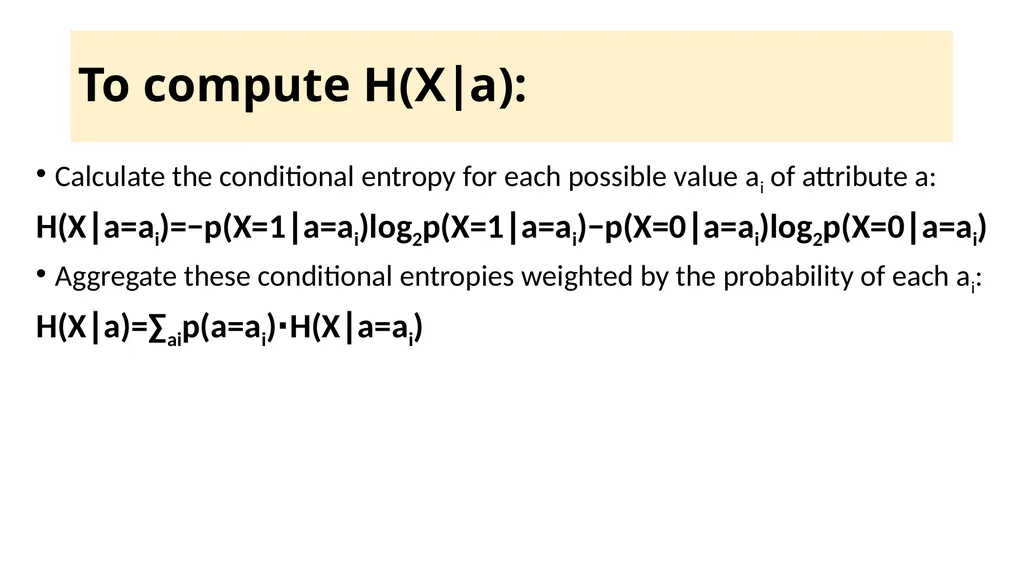
To compute H(X∣a): Calculate the conditional entropy for each possible value ai of attribute a:
H(X∣a=ai)=−p(X=1∣a=ai)log2p(X=1∣a=ai)−p(X=0∣a=ai)log2p(X=0∣a=ai)
Aggregate these conditional entropies weighted by the probability of each ai:
H(X∣a)=∑aip(a=ai)⋅H(X∣a=ai)<br>
H(X∣a=ai)=−p(X=1∣a=ai)log2p(X=1∣a=ai)−p(X=0∣a=ai)log2p(X=0∣a=ai)
Aggregate these conditional entropies weighted by the probability of each ai:
H(X∣a)=∑aip(a=ai)⋅H(X∣a=ai)<br>
74
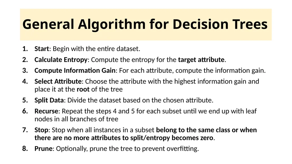
General Algorithm for Decision Trees Start: Begin with the entire dataset.
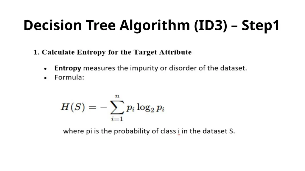
Calculate Entropy: Compute the entropy for the target attribute.
Compute Information Gain: For each attribute, compute the information gain.
Select Attribute: Choose the attribute with the highest information gain and place it at the root of the tree
Split Data: Divide the dataset based on the chosen attribute.
Recurse: Repeat the steps 4 and 5 for each subset until we end up with leaf nodes in all branches of tree
Stop: Stop when all instances in a subset belong to the same class or when there are no more attributes to split/entropy becomes zero.
Prune: Optionally, prune the tree to prevent overfitting.<br>
Calculate Entropy: Compute the entropy for the target attribute.
Compute Information Gain: For each attribute, compute the information gain.
Select Attribute: Choose the attribute with the highest information gain and place it at the root of the tree
Split Data: Divide the dataset based on the chosen attribute.
Recurse: Repeat the steps 4 and 5 for each subset until we end up with leaf nodes in all branches of tree
Stop: Stop when all instances in a subset belong to the same class or when there are no more attributes to split/entropy becomes zero.
Prune: Optionally, prune the tree to prevent overfitting.<br>
75
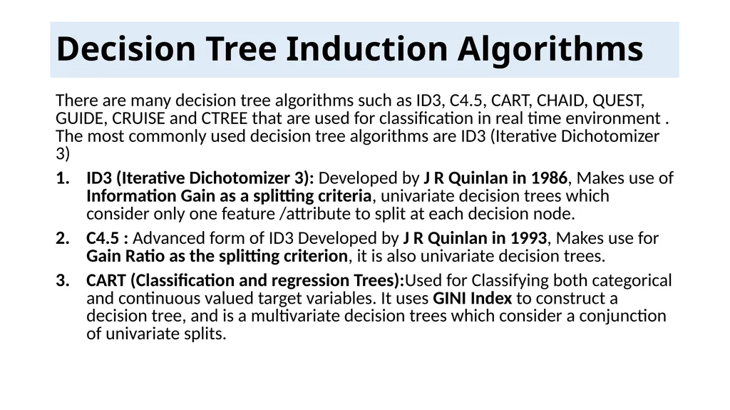
Decision Tree Induction Algorithms There are many decision tree algorithms such as ID3, C4.5, CART, CHAID, QUEST, GUIDE, CRUISE and CTREE that are used for classification in real time environment . The most commonly used decision tree algorithms are ID3 (Iterative Dichotomizer 3)
ID3 (Iterative Dichotomizer 3): Developed by J R Quinlan in 1986, Makes use of Information Gain as a splitting criteria, univariate decision trees which consider only one feature /attribute to split at each decision node.
C4.5 : Advanced form of ID3 Developed by J R Quinlan in 1993, Makes use for Gain Ratio as the splitting criterion, it is also univariate decision trees.
CART (Classification and regression Trees):Used for Classifying both categorical and continuous valued target variables. It uses GINI Index to construct a decision tree, and is a multivariate decision trees which consider a conjunction of univariate splits.<br>
ID3 (Iterative Dichotomizer 3): Developed by J R Quinlan in 1986, Makes use of Information Gain as a splitting criteria, univariate decision trees which consider only one feature /attribute to split at each decision node.
C4.5 : Advanced form of ID3 Developed by J R Quinlan in 1993, Makes use for Gain Ratio as the splitting criterion, it is also univariate decision trees.
CART (Classification and regression Trees):Used for Classifying both categorical and continuous valued target variables. It uses GINI Index to construct a decision tree, and is a multivariate decision trees which consider a conjunction of univariate splits.<br>
76
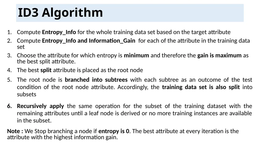
ID3 Algorithm Compute Entropy_Info for the whole training data set based on the target attribute
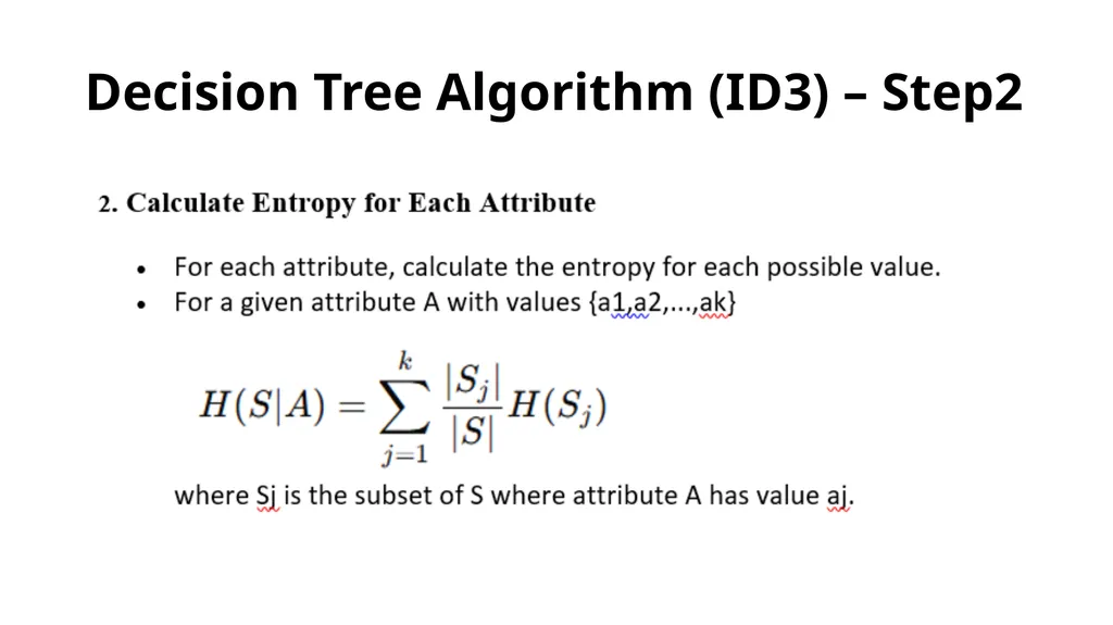
Compute Entropy_Info and Information_Gain for each of the attribute in the training data set
Choose the attribute for which entropy is minimum and therefore the gain is maximum as the best split attribute.
The best split attribute is placed as the root node
The root node is branched into subtrees with each subtree as an outcome of the test condition of the root node attribute. Accordingly, the training data set is also split into subsets
Recursively apply the same operation for the subset of the training dataset with the remaining attributes until a leaf node is derived or no more training instances are available in the subset.
Note : We Stop branching a node if entropy is 0. The best attribute at every iteration is the attribute with the highest information gain.<br>
Compute Entropy_Info and Information_Gain for each of the attribute in the training data set
Choose the attribute for which entropy is minimum and therefore the gain is maximum as the best split attribute.
The best split attribute is placed as the root node
The root node is branched into subtrees with each subtree as an outcome of the test condition of the root node attribute. Accordingly, the training data set is also split into subsets
Recursively apply the same operation for the subset of the training dataset with the remaining attributes until a leaf node is derived or no more training instances are available in the subset.
Note : We Stop branching a node if entropy is 0. The best attribute at every iteration is the attribute with the highest information gain.<br>
77
Decision Tree Algorithm (ID3) – Step1<br>
78
Decision Tree Algorithm (ID3) – Step2<br>
79
Decision Tree Algorithm (ID3) – Step3,Step4<br>
80
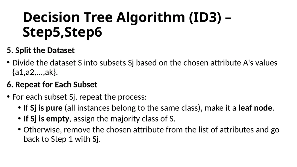
Decision Tree Algorithm (ID3) – Step5,Step6 5. Split the Dataset
Divide the dataset S into subsets Sj based on the chosen attribute A's values {a1,a2,...,ak}.
6. Repeat for Each Subset
For each subset Sj, repeat the process:
If Sj is pure (all instances belong to the same class), make it a leaf node.
If Sj is empty, assign the majority class of S.
Otherwise, remove the chosen attribute from the list of attributes and go back to Step 1 with Sj.<br>
Divide the dataset S into subsets Sj based on the chosen attribute A's values {a1,a2,...,ak}.
6. Repeat for Each Subset
For each subset Sj, repeat the process:
If Sj is pure (all instances belong to the same class), make it a leaf node.
If Sj is empty, assign the majority class of S.
Otherwise, remove the chosen attribute from the list of attributes and go back to Step 1 with Sj.<br>
81
Decision Tree Algorithm (ID3) – Step7 To avoid overfitting, you can prune the tree by removing branches that have little importance. This is usually done by setting a maximum depth or by using cross-validation.<br>
82
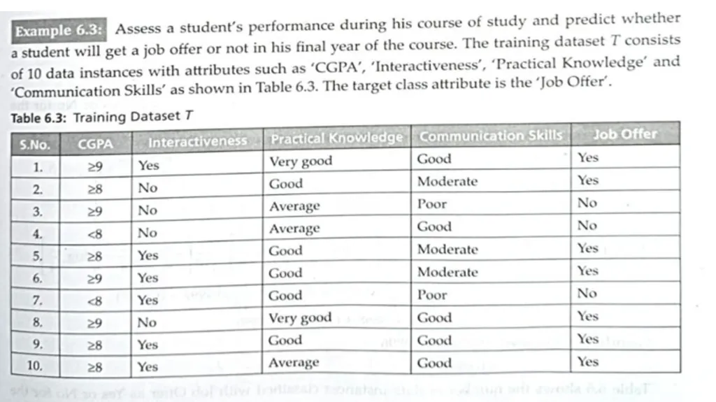
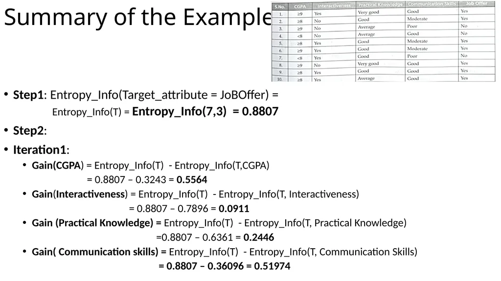
Summary of the Example Step1: Entropy_Info(Target_attribute = JoBOffer) =
Entropy_Info(T) = Entropy_Info(7,3) = 0.8807
Step2:
Iteration1:
Gain(CGPA) = Entropy_Info(T) - Entropy_Info(T,CGPA)
= 0.8807 – 0.3243 = 0.5564
Gain(Interactiveness) = Entropy_Info(T) - Entropy_Info(T, Interactiveness)
= 0.8807 – 0.7896 = 0.0911
Gain (Practical Knowledge) = Entropy_Info(T) - Entropy_Info(T, Practical Knowledge)
=0.8807 – 0.6361 = 0.2446
Gain( Communication skills) = Entropy_Info(T) - Entropy_Info(T, Communication Skills)
= 0.8807 – 0.36096 = 0.51974<br>
Entropy_Info(T) = Entropy_Info(7,3) = 0.8807
Step2:
Iteration1:
Gain(CGPA) = Entropy_Info(T) - Entropy_Info(T,CGPA)
= 0.8807 – 0.3243 = 0.5564
Gain(Interactiveness) = Entropy_Info(T) - Entropy_Info(T, Interactiveness)
= 0.8807 – 0.7896 = 0.0911
Gain (Practical Knowledge) = Entropy_Info(T) - Entropy_Info(T, Practical Knowledge)
=0.8807 – 0.6361 = 0.2446
Gain( Communication skills) = Entropy_Info(T) - Entropy_Info(T, Communication Skills)
= 0.8807 – 0.36096 = 0.51974<br>
83
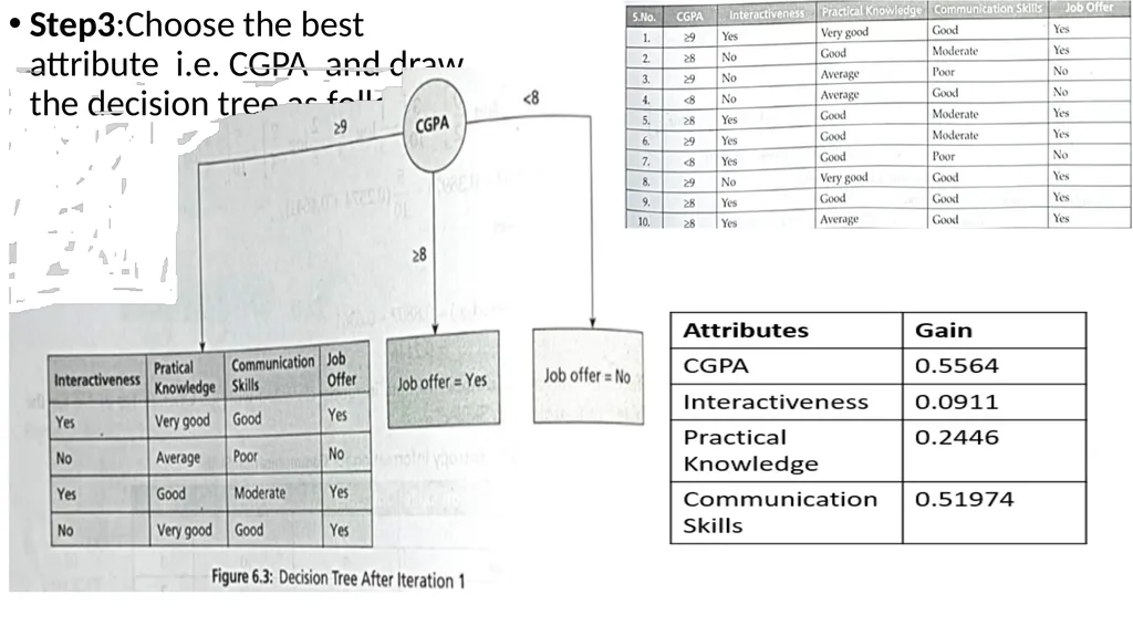
Step3:Choose the best attribute i.e. CGPA and draw the decision tree as follows:<br>
84
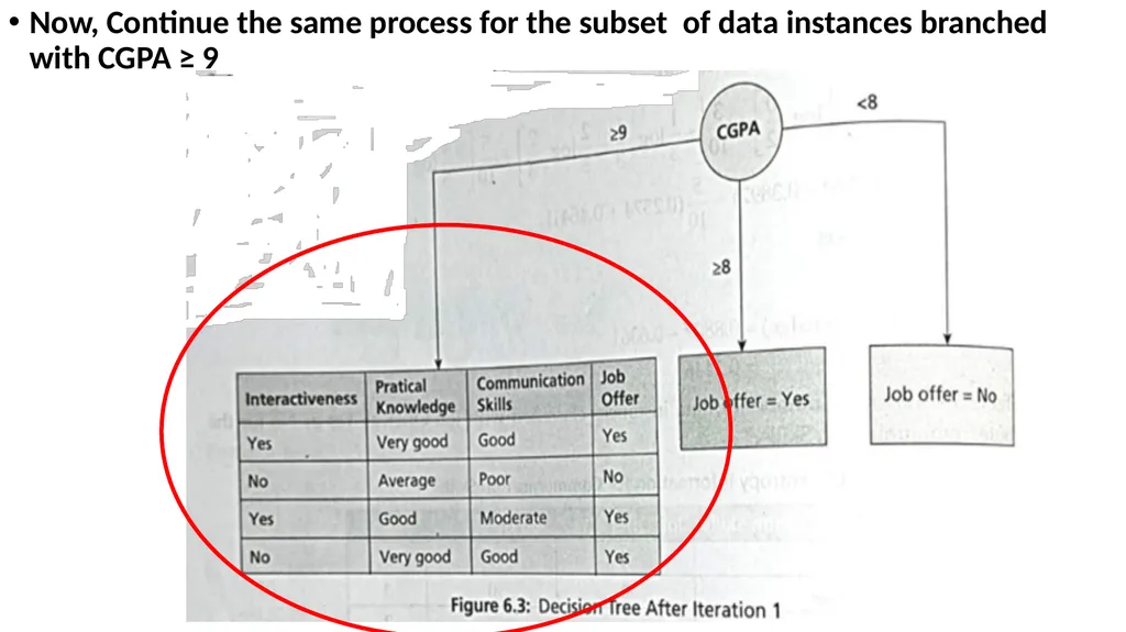
Now, Continue the same process for the subset of data instances branched with CGPA ≥ 9<br>
85
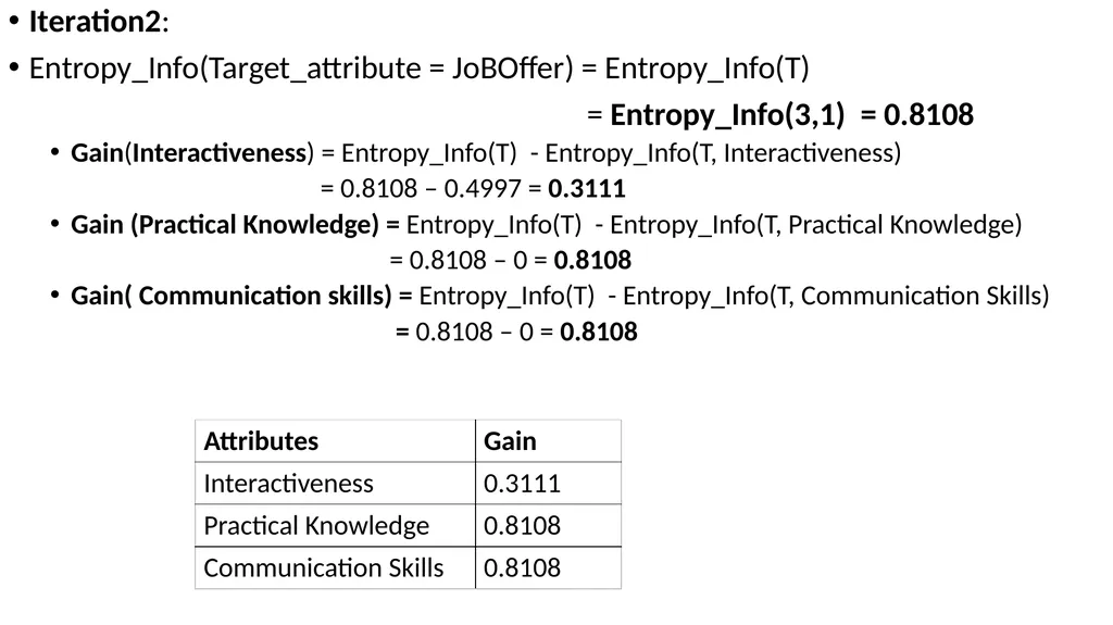
Iteration2:
Entropy_Info(Target_attribute = JoBOffer) = Entropy_Info(T)
= Entropy_Info(3,1) = 0.8108
Gain(Interactiveness) = Entropy_Info(T) - Entropy_Info(T, Interactiveness)
= 0.8108 – 0.4997 = 0.3111
Gain (Practical Knowledge) = Entropy_Info(T) - Entropy_Info(T, Practical Knowledge)
= 0.8108 – 0 = 0.8108
Gain( Communication skills) = Entropy_Info(T) - Entropy_Info(T, Communication Skills)
= 0.8108 – 0 = 0.8108<br>
Entropy_Info(Target_attribute = JoBOffer) = Entropy_Info(T)
= Entropy_Info(3,1) = 0.8108
Gain(Interactiveness) = Entropy_Info(T) - Entropy_Info(T, Interactiveness)
= 0.8108 – 0.4997 = 0.3111
Gain (Practical Knowledge) = Entropy_Info(T) - Entropy_Info(T, Practical Knowledge)
= 0.8108 – 0 = 0.8108
Gain( Communication skills) = Entropy_Info(T) - Entropy_Info(T, Communication Skills)
= 0.8108 – 0 = 0.8108<br>
86
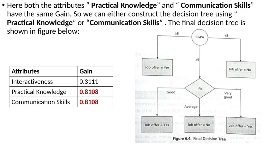
Here both the attributes “ Practical Knowledge” and “ Communication Skills” have the same Gain. So we can either construct the decision tree using “ Practical Knowledge” or “Communication Skills” . The final decision tree is shown in figure below:<br>
87
Handling Continuous Variables in Decision Trees Using Packages that Implement Decision Trees
Building a Decision Tree Algorithm Yourself<br>
Building a Decision Tree Algorithm Yourself<br>
88
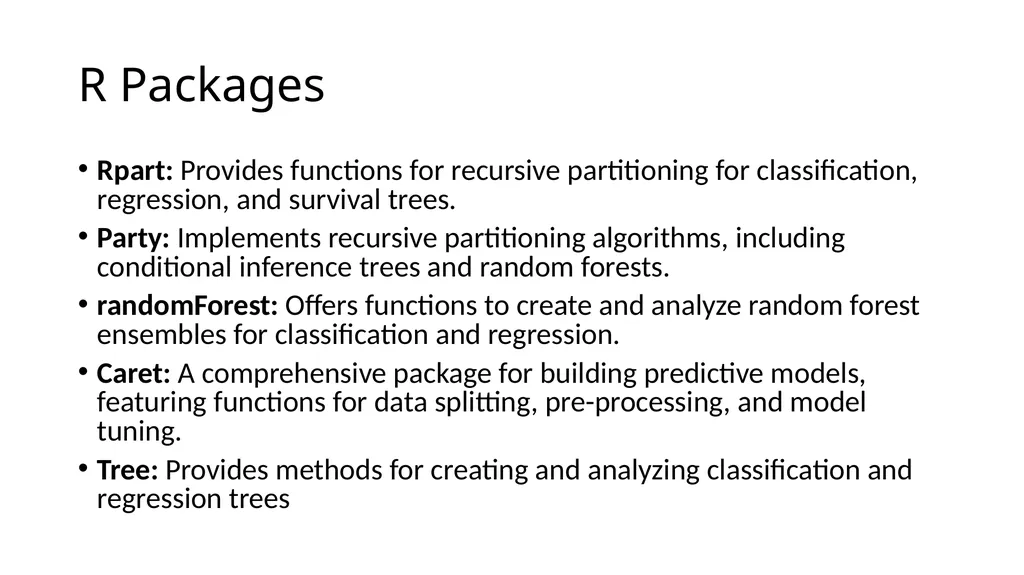
R Packages Rpart: Provides functions for recursive partitioning for classification, regression, and survival trees.
Party: Implements recursive partitioning algorithms, including conditional inference trees and random forests.
randomForest: Offers functions to create and analyze random forest ensembles for classification and regression.
Caret: A comprehensive package for building predictive models, featuring functions for data splitting, pre-processing, and model tuning.
Tree: Provides methods for creating and analyzing classification and regression trees<br>
Party: Implements recursive partitioning algorithms, including conditional inference trees and random forests.
randomForest: Offers functions to create and analyze random forest ensembles for classification and regression.
Caret: A comprehensive package for building predictive models, featuring functions for data splitting, pre-processing, and model tuning.
Tree: Provides methods for creating and analyzing classification and regression trees<br>
89
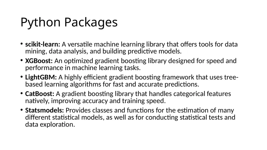
Python Packages scikit-learn: A versatile machine learning library that offers tools for data mining, data analysis, and building predictive models.
XGBoost: An optimized gradient boosting library designed for speed and performance in machine learning tasks.
LightGBM: A highly efficient gradient boosting framework that uses tree-based learning algorithms for fast and accurate predictions.
CatBoost: A gradient boosting library that handles categorical features natively, improving accuracy and training speed.
Statsmodels: Provides classes and functions for the estimation of many different statistical models, as well as for conducting statistical tests and data exploration.<br>
XGBoost: An optimized gradient boosting library designed for speed and performance in machine learning tasks.
LightGBM: A highly efficient gradient boosting framework that uses tree-based learning algorithms for fast and accurate predictions.
CatBoost: A gradient boosting library that handles categorical features natively, improving accuracy and training speed.
Statsmodels: Provides classes and functions for the estimation of many different statistical models, as well as for conducting statistical tests and data exploration.<br>
90
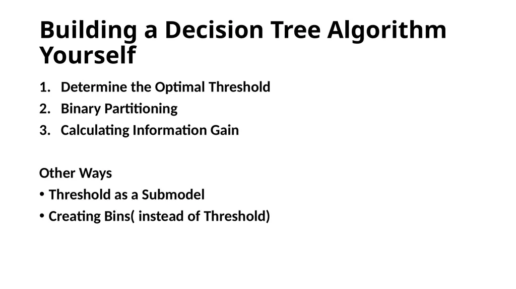
Building a Decision Tree Algorithm Yourself Determine the Optimal Threshold
Binary Partitioning
Calculating Information Gain
Other Ways
Threshold as a Submodel
Creating Bins( instead of Threshold)<br>
Binary Partitioning
Calculating Information Gain
Other Ways
Threshold as a Submodel
Creating Bins( instead of Threshold)<br>
91
Random Forest Random Forest is an ensemble learning method primarily used for classification and regression tasks.
It combines multiple decision trees to produce a more accurate and stable prediction. The key concept behind random forests is to create a 'forest' of decision trees, where each tree is trained on a random subset of the data and features.
The final prediction is made by aggregating the predictions from all individual trees.
Random forests improve decision trees by averaging multiple trees trained on different parts of your data, making your model more accurate and robust, but harder to interpret.
You just need to decide on the number of trees and the number of features to use at each split.<br>
It combines multiple decision trees to produce a more accurate and stable prediction. The key concept behind random forests is to create a 'forest' of decision trees, where each tree is trained on a random subset of the data and features.
The final prediction is made by aggregating the predictions from all individual trees.
Random forests improve decision trees by averaging multiple trees trained on different parts of your data, making your model more accurate and robust, but harder to interpret.
You just need to decide on the number of trees and the number of features to use at each split.<br>
92
Bagging in Random Forest Random forests are an advanced version of decision trees, using a method called bagging (or bootstrap aggregating) to improve accuracy and robustness at the expense of interpretability
Key Points:
Bagging: This technique creates multiple subsets of your data by sampling with replacement. Each subset is used to train a different tree. This helps to reduce variance and avoid overfitting.
Hyperparameters: Random forests are simple to set up with two main hyperparameters:
Number of trees (N): How many trees to include in the forest.
Number of features (F): How many features to randomly select at each split in a tree.
Tree-specific parameters (e.g., max tree depth, min samples per leaf) to optimize performance.<br>
Key Points:
Bagging: This technique creates multiple subsets of your data by sampling with replacement. Each subset is used to train a different tree. This helps to reduce variance and avoid overfitting.
Hyperparameters: Random forests are simple to set up with two main hyperparameters:
Number of trees (N): How many trees to include in the forest.
Number of features (F): How many features to randomly select at each split in a tree.
Tree-specific parameters (e.g., max tree depth, min samples per leaf) to optimize performance.<br>
93
Bootstrapping in Random Forest: A bootstrap sample involves randomly selecting data points with replacement, often using 80% of the dataset.
This introduces a third hyperparameter, the sample size, but it's usually kept constant.<br>
This introduces a third hyperparameter, the sample size, but it's usually kept constant.<br>
94
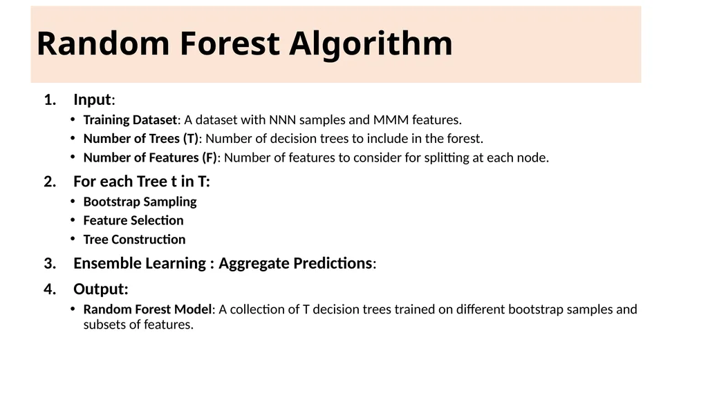
Random Forest Algorithm Input:
Training Dataset: A dataset with NNN samples and MMM features.
Number of Trees (T): Number of decision trees to include in the forest.
Number of Features (F): Number of features to consider for splitting at each node.
For each Tree t in T:
Bootstrap Sampling
Feature Selection
Tree Construction
Ensemble Learning : Aggregate Predictions:
Output:
Random Forest Model: A collection of T decision trees trained on different bootstrap samples and subsets of features.<br>
Training Dataset: A dataset with NNN samples and MMM features.
Number of Trees (T): Number of decision trees to include in the forest.
Number of Features (F): Number of features to consider for splitting at each node.
For each Tree t in T:
Bootstrap Sampling
Feature Selection
Tree Construction
Ensemble Learning : Aggregate Predictions:
Output:
Random Forest Model: A collection of T decision trees trained on different bootstrap samples and subsets of features.<br>
95
User Retention: Interpretability Versus Predictive Power The balance between interpretability and predictive power is important in user retention using decision trees. The key points includes:
Interpretability vs. Predictive Power
Insightful Interpretation
Causal vs. Correlation Understanding
Feature Selection and Testing
Practical Implementation<br>
Interpretability vs. Predictive Power
Insightful Interpretation
Causal vs. Correlation Understanding
Feature Selection and Testing
Practical Implementation<br>
96
David Huffaker: Google’s Hybrid Approach to Social Research Google's Approach to Research and Development
Moving from Descriptive to Predictive Analysis
Insights from Mixed-Methods Research:
Social Layer Integration Across Google Products:
Privacy Concerns and User Engagement:<br>
Moving from Descriptive to Predictive Analysis
Insights from Mixed-Methods Research:
Social Layer Integration Across Google Products:
Privacy Concerns and User Engagement:<br>
97
1. Google's Approach to Research and Development Google integrates research with product development, emphasizing iterative work and early deployment of near-production code .
Researchers collaborate closely with product teams to deploy experiments at scale and conduct iterative testing with smaller user groups<br>
Researchers collaborate closely with product teams to deploy experiments at scale and conduct iterative testing with smaller user groups<br>
98
2. Moving from Descriptive to Predictive Analysis David advocates transitioning from descriptive data analysis to experimental designs that establish causal relationships .
Example: Introduction of Google+'s "circle of friends" feature involved mixed-method approaches to understand user motivations for selective sharing.<br>
Example: Introduction of Google+'s "circle of friends" feature involved mixed-method approaches to understand user motivations for selective sharing.<br>
99
3. Insights from Mixed-Methods Research: Google employed both qualitative (interviews, surveys) and quantitative (data analysis from 100,000 users) methods to study user behavior and preferences [8].
Key findings included user preferences for privacy, relevance, and distribution when sharing content.<br>
Key findings included user preferences for privacy, relevance, and distribution when sharing content.<br>
100
4. Social Layer Integration Across Google Products: Google integrates social elements into various products like Search, incorporating social annotations based on user preferences and domain expertise<br>
101
5. Privacy Concerns and User Engagement: Privacy concerns significantly impact user engagement, highlighting the importance of clear information and control over shared data .
Users are wary of identity theft, unwanted spam, and privacy breaches affecting both digital and physical realms.<br>
Users are wary of identity theft, unwanted spam, and privacy breaches affecting both digital and physical realms.<br>
102
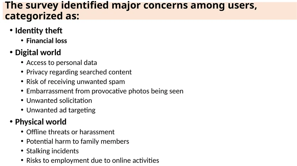
The survey identified major concerns among users, categorized as: Identity theft
Financial loss
Digital world
Access to personal data
Privacy regarding searched content
Risk of receiving unwanted spam
Embarrassment from provocative photos being seen
Unwanted solicitation
Unwanted ad targeting
Physical world
Offline threats or harassment
Potential harm to family members
Stalking incidents
Risks to employment due to online activities<br>
Financial loss
Digital world
Access to personal data
Privacy regarding searched content
Risk of receiving unwanted spam
Embarrassment from provocative photos being seen
Unwanted solicitation
Unwanted ad targeting
Physical world
Offline threats or harassment
Potential harm to family members
Stalking incidents
Risks to employment due to online activities<br>
103
Recommendation Engines: Building a User-Facing Data Product at Scale Recommendation engines, also known as recommendation systems, are a prime example of data products. Example : Amazon and Netflix.
These systems use data generated by users, such as book purchases or movie ratings, to provide personalized recommendations.
This process involves complex engineering and algorithms, requiring knowledge of linear algebra and coding.
Building such systems highlights the challenges of handling Big Data and implementing scalable solutions.<br>
These systems use data generated by users, such as book purchases or movie ratings, to provide personalized recommendations.
This process involves complex engineering and algorithms, requiring knowledge of linear algebra and coding.
Building such systems highlights the challenges of handling Big Data and implementing scalable solutions.<br>
104
Matt Gattis, Experience In this context, Matt Gattis, an MIT graduate and co-founder of Hunch.com, shares his experience in building a recommendation system for the site. Hunch.com.
Initially asked users a series of questions to provide personalized advice on various topics, using machine learning to improve recommendations over time.
They found that answering 20 questions could predict additional user preferences with 80% accuracy, involving traits similar to those assessed by the Myers-Briggs Type Indicator (MBTI).<br>
Initially asked users a series of questions to provide personalized advice on various topics, using machine learning to improve recommendations over time.
They found that answering 20 questions could predict additional user preferences with 80% accuracy, involving traits similar to those assessed by the Myers-Briggs Type Indicator (MBTI).<br>
105
Matt Gattis, Experience Hunch later shifted to an API model, gathering data from the web and allowing third parties to use their service to personalize content.
This business model led to eBay acquiring Hunch.<br>
This business model led to eBay acquiring Hunch.<br>
106
A Real-World Recommendation Engine Recommendation engines are ubiquitous, suggesting movies, books, and vacations based on users' past preferences.
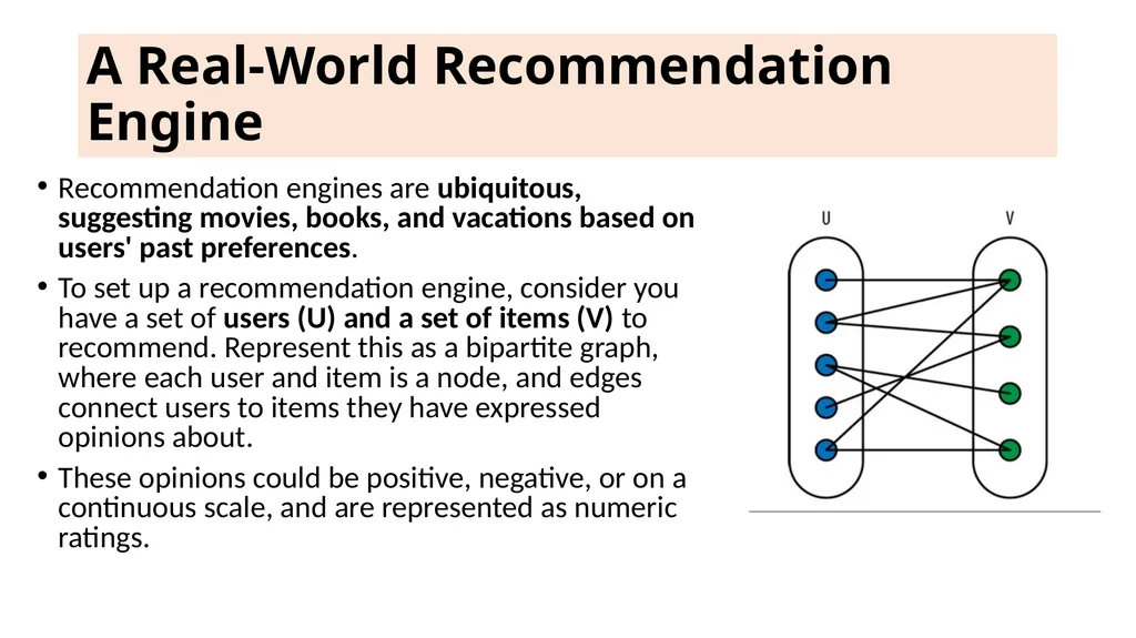
To set up a recommendation engine, consider you have a set of users (U) and a set of items (V) to recommend. Represent this as a bipartite graph, where each user and item is a node, and edges connect users to items they have expressed opinions about.
These opinions could be positive, negative, or on a continuous scale, and are represented as numeric ratings.<br>
To set up a recommendation engine, consider you have a set of users (U) and a set of items (V) to recommend. Represent this as a bipartite graph, where each user and item is a node, and edges connect users to items they have expressed opinions about.
These opinions could be positive, negative, or on a continuous scale, and are represented as numeric ratings.<br>
107
A Real-World Recommendation Engine Using training data that includes known preferences of some users for some items, the goal is to predict other preferences for these users.
Additional metadata on users (e.g., gender, age) or items (e.g., color) can also be incorporated.
Users can be represented as vectors of features, which might include preferences depending on the context.
All user vectors can be combined into a large user matrix, denoted as U.<br>
Additional metadata on users (e.g., gender, age) or items (e.g., color) can also be incorporated.
Users can be represented as vectors of features, which might include preferences depending on the context.
All user vectors can be combined into a large user matrix, denoted as U.<br>
108
Using Nearest Neighbour Algorithm for recommendation Purpose: To find the item(s) most similar to a given item based on certain features or characteristics.
Steps:
Data Preparation
Choose a Distance Metric
Calculate Distance
Find Nearest Neighbors
Recommendation<br>
Steps:
Data Preparation
Choose a Distance Metric
Calculate Distance
Find Nearest Neighbors
Recommendation<br>
109
Example: Let's say you want to recommend movies based on a user's previous movie ratings.<br>
110
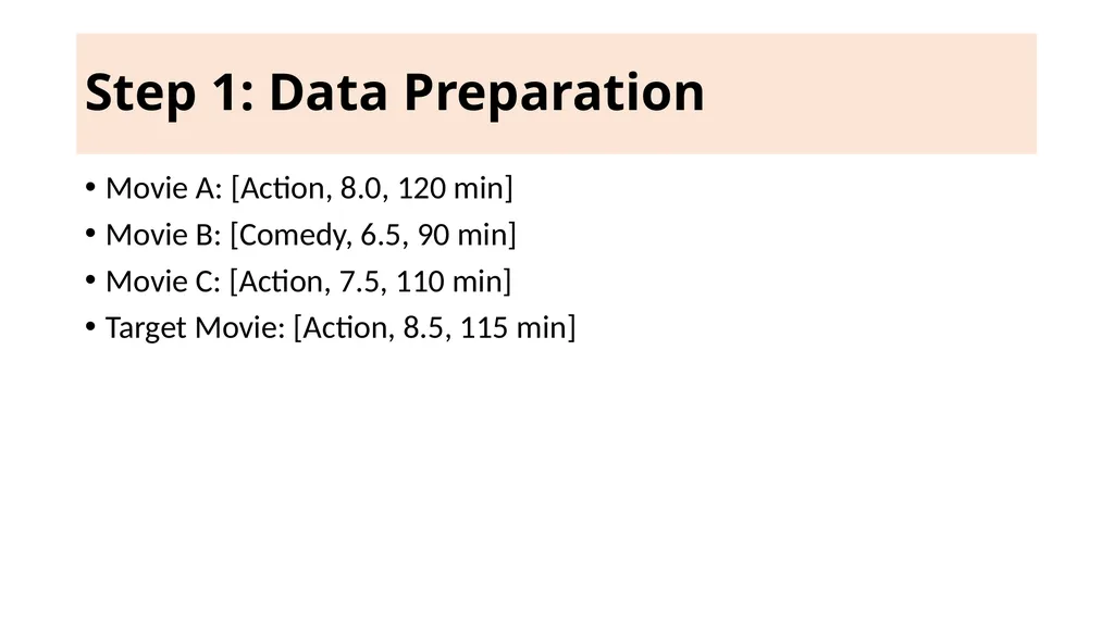
Step 1: Data Preparation Movie A: [Action, 8.0, 120 min]
Movie B: [Comedy, 6.5, 90 min]
Movie C: [Action, 7.5, 110 min]
Target Movie: [Action, 8.5, 115 min]<br>
Movie B: [Comedy, 6.5, 90 min]
Movie C: [Action, 7.5, 110 min]
Target Movie: [Action, 8.5, 115 min]<br>
111
Step 2: Choose a Distance Metric • We'll use Euclidean distance<br>
112
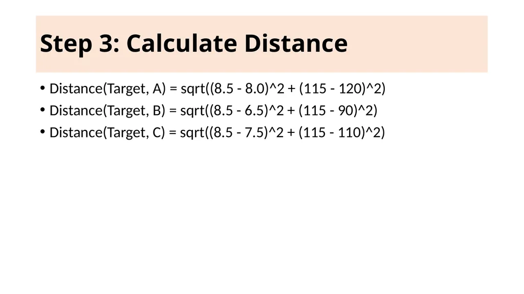
Step 3: Calculate Distance Distance(Target, A) = sqrt((8.5 - 8.0)^2 + (115 - 120)^2)
Distance(Target, B) = sqrt((8.5 - 6.5)^2 + (115 - 90)^2)
Distance(Target, C) = sqrt((8.5 - 7.5)^2 + (115 - 110)^2)<br>
Distance(Target, B) = sqrt((8.5 - 6.5)^2 + (115 - 90)^2)
Distance(Target, C) = sqrt((8.5 - 7.5)^2 + (115 - 110)^2)<br>
113
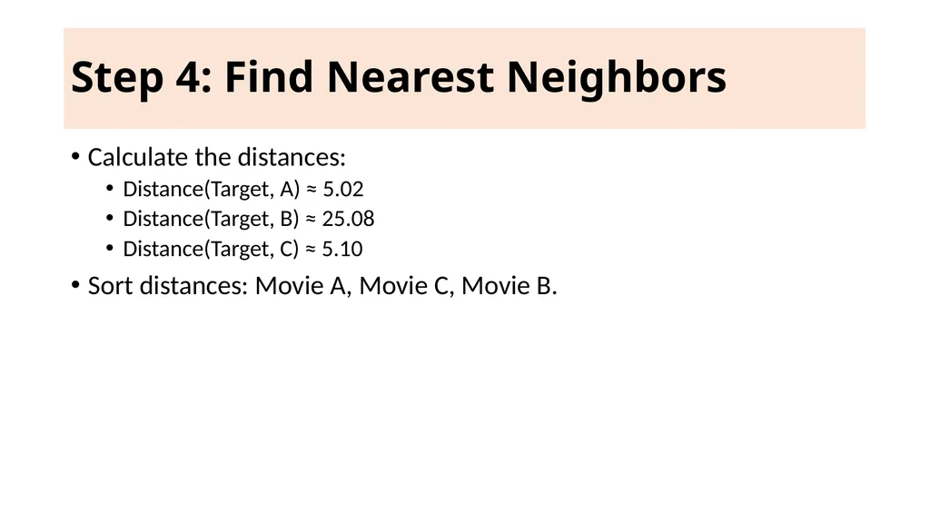
Step 4: Find Nearest Neighbors Calculate the distances:
Distance(Target, A) ≈ 5.02
Distance(Target, B) ≈ 25.08
Distance(Target, C) ≈ 5.10
Sort distances: Movie A, Movie C, Movie B.<br>
Distance(Target, A) ≈ 5.02
Distance(Target, B) ≈ 25.08
Distance(Target, C) ≈ 5.10
Sort distances: Movie A, Movie C, Movie B.<br>
114
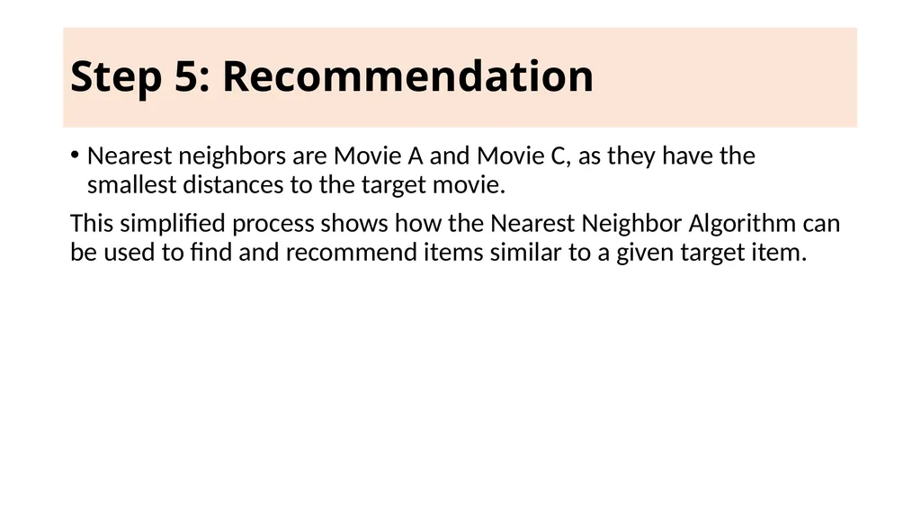
Step 5: Recommendation Nearest neighbors are Movie A and Movie C, as they have the smallest distances to the target movie.
This simplified process shows how the Nearest Neighbor Algorithm can be used to find and recommend items similar to a given target item.<br>
This simplified process shows how the Nearest Neighbor Algorithm can be used to find and recommend items similar to a given target item.<br>
115
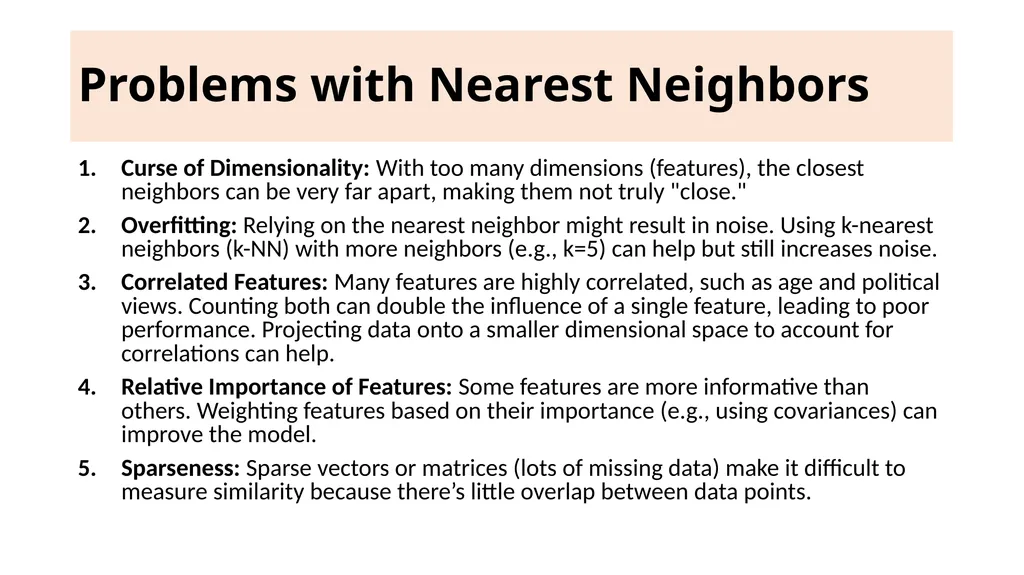
Problems with Nearest Neighbors Curse of Dimensionality: With too many dimensions (features), the closest neighbors can be very far apart, making them not truly "close."
Overfitting: Relying on the nearest neighbor might result in noise. Using k-nearest neighbors (k-NN) with more neighbors (e.g., k=5) can help but still increases noise.
Correlated Features: Many features are highly correlated, such as age and political views. Counting both can double the influence of a single feature, leading to poor performance. Projecting data onto a smaller dimensional space to account for correlations can help.
Relative Importance of Features: Some features are more informative than others. Weighting features based on their importance (e.g., using covariances) can improve the model.
Sparseness: Sparse vectors or matrices (lots of missing data) make it difficult to measure similarity because there’s little overlap between data points.<br>
Overfitting: Relying on the nearest neighbor might result in noise. Using k-nearest neighbors (k-NN) with more neighbors (e.g., k=5) can help but still increases noise.
Correlated Features: Many features are highly correlated, such as age and political views. Counting both can double the influence of a single feature, leading to poor performance. Projecting data onto a smaller dimensional space to account for correlations can help.
Relative Importance of Features: Some features are more informative than others. Weighting features based on their importance (e.g., using covariances) can improve the model.
Sparseness: Sparse vectors or matrices (lots of missing data) make it difficult to measure similarity because there’s little overlap between data points.<br>
116
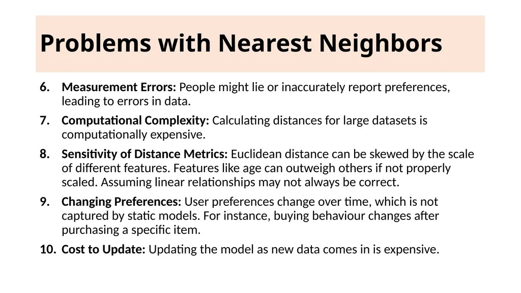
Problems with Nearest Neighbors Measurement Errors: People might lie or inaccurately report preferences, leading to errors in data.
Computational Complexity: Calculating distances for large datasets is computationally expensive.
Sensitivity of Distance Metrics: Euclidean distance can be skewed by the scale of different features. Features like age can outweigh others if not properly scaled. Assuming linear relationships may not always be correct.
Changing Preferences: User preferences change over time, which is not captured by static models. For instance, buying behaviour changes after purchasing a specific item.
Cost to Update: Updating the model as new data comes in is expensive.<br>
Computational Complexity: Calculating distances for large datasets is computationally expensive.
Sensitivity of Distance Metrics: Euclidean distance can be skewed by the scale of different features. Features like age can outweigh others if not properly scaled. Assuming linear relationships may not always be correct.
Changing Preferences: User preferences change over time, which is not captured by static models. For instance, buying behaviour changes after purchasing a specific item.
Cost to Update: Updating the model as new data comes in is expensive.<br>
117
Key Issues The primary problems are overfitting and the curse of dimensionality.
Addressing these involves thinking about more robust methods, potentially drawing from familiar techniques like linear regression.<br>
Addressing these involves thinking about more robust methods, potentially drawing from familiar techniques like linear regression.<br>
118
Beyond Nearest Neighbor: Machine Learning Classification To improve recommendation systems beyond nearest neighbors, we can use machine learning, specifically linear regression models for each item.<br>
119
Linear Regression Models for Recommendations Separate Models for Each Item:
Build a distinct linear regression model for each item.
Predict whether a user would like an item based on their attributes (e.g., age, gender).
Incorporate Metadata:
Treat user attributes (metadata) as features in the model.
This allows predicting user preferences even when some attributes are missing.<br>
Build a distinct linear regression model for each item.
Predict whether a user would like an item based on their attributes (e.g., age, gender).
Incorporate Metadata:
Treat user attributes (metadata) as features in the model.
This allows predicting user preferences even when some attributes are missing.<br>
120
Example: For a user with three attributes (fi1, fi2, fi3), estimate their preference (pi) for an item using:
pi=β1fi1+β2fi2+β3fi3+ϵ<br>
pi=β1fi1+β2fi2+β3fi3+ϵ<br>
121
Advantages: Feature Weighting: Linear regression inherently solves the feature weighting problem by determining the importance of each feature through its coefficients<br>
122
Challenges: One Model per Item:
Requires as many models as there are items.
Doesn't leverage information from other items.
Overfitting:
Large coefficients can indicate overfitting, especially with limited data.
Overfitting occurs when the model captures noise rather than the underlying pattern.<br>
Requires as many models as there are items.
Doesn't leverage information from other items.
Overfitting:
Large coefficients can indicate overfitting, especially with limited data.
Overfitting occurs when the model captures noise rather than the underlying pattern.<br>
123
Addressing Overfitting: Impose a Bayesian Prior: Add a penalty term to the regression to prevent large coefficients. The penalty term depends on a parameter, λ (lambda).
Choosing λ: Experimentally adjust λ by evaluating model performance on a training set.
Normalization: Normalize variables to ensure that coefficients have reasonable sizes.<br>
Choosing λ: Experimentally adjust λ by evaluating model performance on a training set.
Normalization: Normalize variables to ensure that coefficients have reasonable sizes.<br>
124
Normalization: Normalize variables to ensure that coefficients have reasonable sizes.
Different normalization methods can be applied if certain variables are expected to have larger coefficients.<br>
Different normalization methods can be applied if certain variables are expected to have larger coefficients.<br>
125
The Dimensionality Problem The dimensionality problem in data analysis refers to dealing with a large number of items or features, often tens of thousands.
To manage this, techniques like Singular Value Decomposition (SVD) and Principal Component Analysis (PCA) are commonly used.<br>
To manage this, techniques like Singular Value Decomposition (SVD) and Principal Component Analysis (PCA) are commonly used.<br>
126
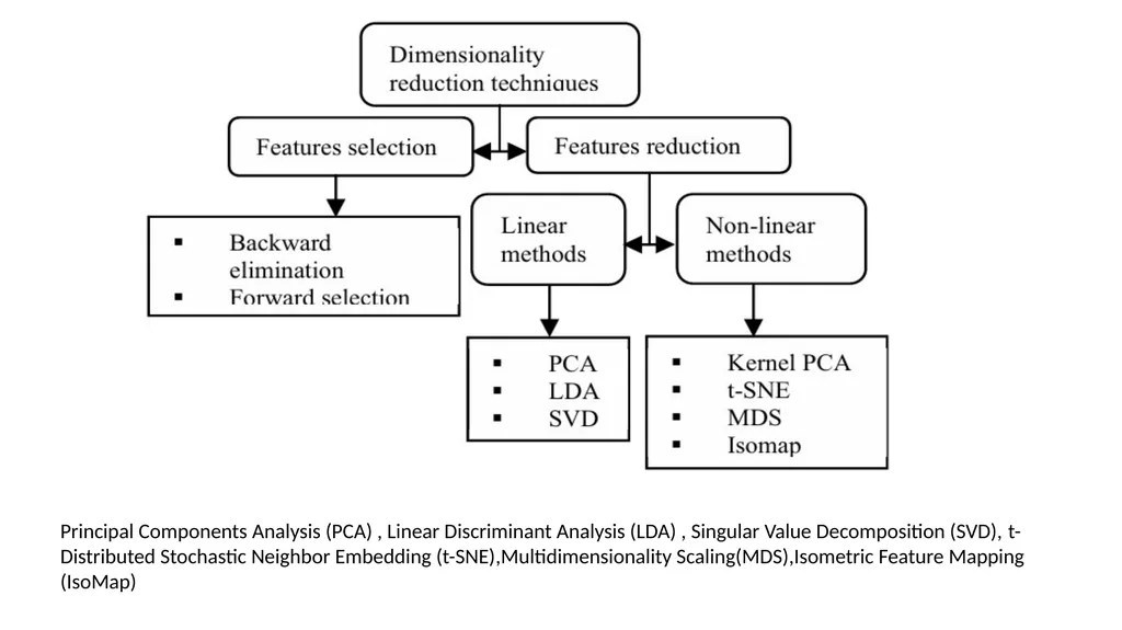
Principal Components Analysis (PCA) , Linear Discriminant Analysis (LDA) , Singular Value Decomposition (SVD), t-Distributed Stochastic Neighbor Embedding (t-SNE),Multidimensionality Scaling(MDS),Isometric Feature Mapping (IsoMap)<br>
127
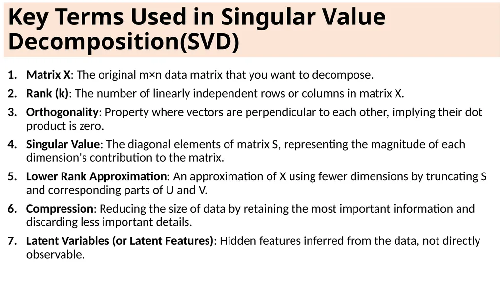
Key Terms Used in Singular Value Decomposition(SVD) Matrix X: The original m×n data matrix that you want to decompose.
Rank (k): The number of linearly independent rows or columns in matrix X.
Orthogonality: Property where vectors are perpendicular to each other, implying their dot product is zero.
Singular Value: The diagonal elements of matrix S, representing the magnitude of each dimension's contribution to the matrix.
Lower Rank Approximation: An approximation of X using fewer dimensions by truncating S and corresponding parts of U and V.
Compression: Reducing the size of data by retaining the most important information and discarding less important details.
Latent Variables (or Latent Features): Hidden features inferred from the data, not directly observable.<br>
Rank (k): The number of linearly independent rows or columns in matrix X.
Orthogonality: Property where vectors are perpendicular to each other, implying their dot product is zero.
Singular Value: The diagonal elements of matrix S, representing the magnitude of each dimension's contribution to the matrix.
Lower Rank Approximation: An approximation of X using fewer dimensions by truncating S and corresponding parts of U and V.
Compression: Reducing the size of data by retaining the most important information and discarding less important details.
Latent Variables (or Latent Features): Hidden features inferred from the data, not directly observable.<br>
128
Key Terms Used in Singular Value Decomposition(SVD) U Matrix: An m×k matrix whose columns are orthogonal and represent the left singular vectors.
S Matrix: A k×k diagonal matrix containing singular values, ordered by magnitude.
V Matrix: An n×k matrix whose columns are orthogonal and represent the right singular vectors.
Eigenvalues and Eigenvectors: Eigenvalues are scalars indicating the variance explained by each dimension, and eigenvectors are the directions of these dimensions.
Unitary Matrix: A matrix whose inverse is equal to its transpose.
Dimensionality Reduction: The process of reducing the number of random variables under consideration by obtaining a set of principal variables.
Base Change Operation: Reordering columns based on the magnitude of singular values.<br>
S Matrix: A k×k diagonal matrix containing singular values, ordered by magnitude.
V Matrix: An n×k matrix whose columns are orthogonal and represent the right singular vectors.
Eigenvalues and Eigenvectors: Eigenvalues are scalars indicating the variance explained by each dimension, and eigenvectors are the directions of these dimensions.
Unitary Matrix: A matrix whose inverse is equal to its transpose.
Dimensionality Reduction: The process of reducing the number of random variables under consideration by obtaining a set of principal variables.
Base Change Operation: Reordering columns based on the magnitude of singular values.<br>
129
Key Terms Used in Singular Value Decomposition(SVD) Approximation X: The matrix obtained by multiplying U, S, and V τ back together, serving as an approximation of the original X.
Prediction: Using the approximated X matrix to predict missing or new values in the dataset.
Frobenius Norm: A measure of matrix error used to quantify the difference between the original matrix and its approximation.
Diagonal Matrix: A matrix in which the entries outside the main diagonal are all zero.
Reconstruction: The process of multiplying U, S, and Vτ to get an approximated version of X.
Computational Complexity: The amount of computational resources required to perform SVD, especially significant for large matrices.
SVD-based Recommendations: Using SVD to decompose user-item rating matrices to make personalized recommendations.<br>
Prediction: Using the approximated X matrix to predict missing or new values in the dataset.
Frobenius Norm: A measure of matrix error used to quantify the difference between the original matrix and its approximation.
Diagonal Matrix: A matrix in which the entries outside the main diagonal are all zero.
Reconstruction: The process of multiplying U, S, and Vτ to get an approximated version of X.
Computational Complexity: The amount of computational resources required to perform SVD, especially significant for large matrices.
SVD-based Recommendations: Using SVD to decompose user-item rating matrices to make personalized recommendations.<br>
130
Understanding Dimension Reduction and Latent Features Concept of Latent Features: Latent features are unobserved and not directly measurable.
Dimensionality Reduction: This process simplifies data into fewer dimensions, focusing on essential features.<br>
Dimensionality Reduction: This process simplifies data into fewer dimensions, focusing on essential features.<br>
131
Algorithmic Approach Machine Learning Role
Low Dimensional Subspace<br>
Low Dimensional Subspace<br>
132
Handling Binary Rating Questions Separate Variables for Each Question
Comparison Questions<br>
Comparison Questions<br>
133
SVD: Concept and Mathematical Foundation Singular Value Decomposition (SVD) is a method to decompose any m×n matrix X of rank k into three specific matrices: X=USVτ
U: An m×k matrix with pairwise orthogonal columns.
S : A k×k diagonal matrix.
V: A k×n matrix with pairwise orthogonal columns.<br>
U: An m×k matrix with pairwise orthogonal columns.
S : A k×k diagonal matrix.
V: A k×n matrix with pairwise orthogonal columns.<br>
134
SVD: Application to Data Sets X: Represents the original dataset (e.g., users' ratings of items) with m users and n items.
Rank k: Determines the maximum number of latent variables d to consider.
Tuning Parameter d: Similar to k in k-NN, d is chosen based on the dataset and serves as a tuning parameter for the model.<br>
Rank k: Determines the maximum number of latent variables d to consider.
Tuning Parameter d: Similar to k in k-NN, d is chosen based on the dataset and serves as a tuning parameter for the model.<br>
135
SVD: Interpretation of Matrices U: Each row corresponds to a user.
V: Each row corresponds to an item.
Singular Values in S: Diagonal values in S indicate the importance of each latent variable, with the largest value representing the most critical latent variable.<br>
V: Each row corresponds to an item.
Singular Values in S: Diagonal values in S indicate the importance of each latent variable, with the largest value representing the most critical latent variable.<br>
136
SVD Algorithm<br>
137
SVD Algorithm<br>
138
SVD Algorithm<br>
139
Example: Finding SVD for a Given Matrix<br>
140
Example: Finding SVD for a Given Matrix<br>
141
Example: Finding SVD for a Given Matrix<br>
142
Example: Finding SVD for a Given Matrix<br>
143
Example: Finding SVD for a Given Matrix<br>
144
Example: Finding SVD for a Given Matrix<br>
145
Example: Row Reduced Form<br>
146
Example Computing v1<br>
147
Example : Compute u1<br>
148
Example : Compute u2<br>
149
Example : Compute u2<br>
150
Example : Find a vector which is perpendicular to both vector A and B, where A=2i+3j+4k B=i+2j+3k?<br>
151
Example : Find a vector which is perpendicular to both vector A and B, where A=2i+3j+4k B=i+2j+3k?<br>
152
Important Properties of SVD Orthogonality : The columns of matrices U and V are orthogonal.
Lower Rank Approximation: Lower-rank approximation of matrix X is achieved by truncating S to include only the top singular values and the corresponding parts of U and V.
Compression: This truncation process is a form of data compression, retaining the most significant features and discarding the least important ones.
Choosing Latent Variables d : By selecting a smaller number of latent variables d (where d<k), the approximation retains the essential structure of X while reducing its dimensionality.
Interpretation of U and V: The matrices U and V reveal latent features in the data. For example, the most significant latent feature might differentiate between males and females.<br>
Lower Rank Approximation: Lower-rank approximation of matrix X is achieved by truncating S to include only the top singular values and the corresponding parts of U and V.
Compression: This truncation process is a form of data compression, retaining the most significant features and discarding the least important ones.
Choosing Latent Variables d : By selecting a smaller number of latent variables d (where d<k), the approximation retains the essential structure of X while reducing its dimensionality.
Interpretation of U and V: The matrices U and V reveal latent features in the data. For example, the most significant latent feature might differentiate between males and females.<br>
153
Limitations and Challenges Missing Data: SVD does not inherently solve the issue of missing data.
Computational Complexity: SVD is computationally expensive, making it challenging for large datasets.<br>
Computational Complexity: SVD is computationally expensive, making it challenging for large datasets.<br>
154
Example :Using SVD for Recommendations Initial Data: Suppose you have a user-item rating matrix X with some missing values.
Fill Missing Values: Replace missing values with the average rating for each item.
Compute SVD: Decompose X into U, S, and VT.
Make Predictions: Multiply U, S, and VT to get an approximation of X, and use this approximated matrix to predict ratings for user-item pairs.<br>
Fill Missing Values: Replace missing values with the average rating for each item.
Compute SVD: Decompose X into U, S, and VT.
Make Predictions: Multiply U, S, and VT to get an approximation of X, and use this approximated matrix to predict ratings for user-item pairs.<br>
155
Introduction to Principal Component Analysis (PCA) Principal Component Analysis (PCA) is a technique used to simplify complex data.
It reduces the number of dimensions (or features) in a dataset while preserving as much important information as possible.
This makes it easier to visualize, analyze, and use the data.<br>
It reduces the number of dimensions (or features) in a dataset while preserving as much important information as possible.
This makes it easier to visualize, analyze, and use the data.<br>
156
Here's how PCA works in simple terms: Data Simplification: Imagine you have a dataset with many features (e.g., height, weight, age, income). PCA helps to reduce this to a smaller set of new features that still capture the essential information.
Finding Principal Components: PCA identifies new features called "principal components." These are combinations of the original features that explain the most variance (differences) in the data. The first principal component captures the most variance, the second captures the next most, and so on.
Transformation: The original data is transformed into a new set of uncorrelated features (principal components). These new features are easier to work with because they are not redundant and capture the most important patterns in the data.
Dimensionality Reduction: By selecting a few principal components, you can reduce the number of features while retaining most of the important information. This makes the data simpler and faster to process without losing significant insights.<br>
Finding Principal Components: PCA identifies new features called "principal components." These are combinations of the original features that explain the most variance (differences) in the data. The first principal component captures the most variance, the second captures the next most, and so on.
Transformation: The original data is transformed into a new set of uncorrelated features (principal components). These new features are easier to work with because they are not redundant and capture the most important patterns in the data.
Dimensionality Reduction: By selecting a few principal components, you can reduce the number of features while retaining most of the important information. This makes the data simpler and faster to process without losing significant insights.<br>
157
Why Use PCA? Simplification: Makes complex data easier to understand and visualize.
Efficiency: Reduces computational resources needed for analysis and modeling.
Noise Reduction: Helps to remove less important information and focus on the most critical aspects of the data.
Uncorrelated Features: Ensures that the new features are not redundant, which can improve the performance of machine learning model
In summary, PCA is a powerful tool for simplifying data by finding and using new features that capture the most important information from the original dataset.<br>
Efficiency: Reduces computational resources needed for analysis and modeling.
Noise Reduction: Helps to remove less important information and focus on the most critical aspects of the data.
Uncorrelated Features: Ensures that the new features are not redundant, which can improve the performance of machine learning model
In summary, PCA is a powerful tool for simplifying data by finding and using new features that capture the most important information from the original dataset.<br>
158
Principal Component Analysis (PCA) for Predicting Preferences Approximate the original data matrix X through the product X≈U⋅VT.
Minimize the discrepancy between the actual data X and the predicted data U⋅VT, measured by the squared error:<br>
Minimize the discrepancy between the actual data X and the predicted data U⋅VT, measured by the squared error:<br>
159
Algorithm Steps: Initialization
Optimization Problem
Alternating Least Squares (ALS):
Step 1: Fix V and update U.
Step 2: Fix U and update V.
Convergence Check<br>
Optimization Problem
Alternating Least Squares (ALS):
Step 1: Fix V and update U.
Step 2: Fix U and update V.
Convergence Check<br>
160
1. Initialization Define the number of latent features d. Typically, d is around 100.
Initialize matrices U(of size m×d) and V (of size n×d) with random values, where m is the number of users and n is the number of items.<br>
Initialize matrices U(of size m×d) and V (of size n×d) with random values, where m is the number of users and n is the number of items.<br>
161
2. Optimization Problem<br>
162
3.Alternating Least Squares (ALS): Step 1: Fix V and update U.<br>
163
3.Alternating Least Squares (ALS): Step2: Fix U and update V.<br>
164
4. Convergence Check Repeat the ALS steps until the changes in U and V are smaller than a predefined threshold ϵ.
Once the changes are less than ϵ, the algorithm is considered to have "converged."<br>
Once the changes are less than ϵ, the algorithm is considered to have "converged."<br>
165
Python Inbuilt Libraries Used math
numpy<br>
numpy<br>
166
math Purpose: Provides mathematical functions.Key
Functions: math.sqrt(x): Returns the square root of x.
Usage in Code: To calculate the root mean squared error (RMSE)
Example1 :
import math
result = math.sqrt(16) # result will be 4.0
Example2:
import math
# Calculating root mean squared error
error = math.sqrt(total_error / number_of_elements)<br>
Functions: math.sqrt(x): Returns the square root of x.
Usage in Code: To calculate the root mean squared error (RMSE)
Example1 :
import math
result = math.sqrt(16) # result will be 4.0
Example2:
import math
# Calculating root mean squared error
error = math.sqrt(total_error / number_of_elements)<br>
167
numpy Purpose: Array and matrix operations, linear algebra. Supports large, multi-dimensional arrays and matrices, along with a collection of mathematical functions to operate on these arrays.
Key Functions:
numpy.mat(data): Creates a matrix from an array-like object or a string of data.
numpy.zeros(shape): Returns a new array of given shape and type, filled with zeros.
numpy.eye(N): Returns a 2-D array with ones on the diagonal and zeros elsewhere.
numpy.linalg.inv(a): Computes the (multiplicative) inverse of a matrix.
numpy.vstack(tup): Stacks arrays in sequence vertically (row wise).
Usage in Code: For creating and manipulating matrices and performing linear algebra operations.<br>
Key Functions:
numpy.mat(data): Creates a matrix from an array-like object or a string of data.
numpy.zeros(shape): Returns a new array of given shape and type, filled with zeros.
numpy.eye(N): Returns a 2-D array with ones on the diagonal and zeros elsewhere.
numpy.linalg.inv(a): Computes the (multiplicative) inverse of a matrix.
numpy.vstack(tup): Stacks arrays in sequence vertically (row wise).
Usage in Code: For creating and manipulating matrices and performing linear algebra operations.<br>
168
Example: import numpy
# Creating a matrix
V = numpy.mat([[0.15968384, 0.9441198, 0.83651085],
[0.73573009, 0.24906915, 0.85338239],
[0.25605814, 0.6990532, 0.50900407]])
# Creating a zero matrix
U = numpy.mat(numpy.zeros([6, 3]))
# Identity matrix for regularization
L_identity = L * numpy.mat(numpy.eye(3))
# Inverting a matrix
inv_matrix = numpy.linalg.inv(some_matrix)<br>
# Creating a matrix
V = numpy.mat([[0.15968384, 0.9441198, 0.83651085],
[0.73573009, 0.24906915, 0.85338239],
[0.25605814, 0.6990532, 0.50900407]])
# Creating a zero matrix
U = numpy.mat(numpy.zeros([6, 3]))
# Identity matrix for regularization
L_identity = L * numpy.mat(numpy.eye(3))
# Inverting a matrix
inv_matrix = numpy.linalg.inv(some_matrix)<br>
169
Building a Recommendation System: Sample Code Explanation This sample code demonstrates a basic implementation of a collaborative filtering recommendation system using matrix factorization.
The code is written in Python and utilizes the NumPy library for efficient matrix operations.<br>
The code is written in Python and utilizes the NumPy library for efficient matrix operations.<br>
170
Key aspects of the code: Purpose: To illustrate how to build a recommendation system on a small dataset.
Technique: Matrix factorization, which is a common approach in collaborative filtering.
Data representation: User-item interactions are represented as sparse matrices.
Core idea: The algorithm learns latent features for both users and items, which can then be used to predict ratings.
Iterative approach: The code uses an iterative process to refine the user and item feature matrices, gradually improving the prediction accuracy.
Error measurement: After each iteration, the code calculates the Root Mean Square Error (RMSE) to track the model's performance.<br>
Technique: Matrix factorization, which is a common approach in collaborative filtering.
Data representation: User-item interactions are represented as sparse matrices.
Core idea: The algorithm learns latent features for both users and items, which can then be used to predict ratings.
Iterative approach: The code uses an iterative process to refine the user and item feature matrices, gradually improving the prediction accuracy.
Error measurement: After each iteration, the code calculates the Root Mean Square Error (RMSE) to track the model's performance.<br>
171
Importing Libraries import math
import numpy<br>
import numpy<br>
172
Input Data Structure - User-Item Interactions (pu) pu: List of tuples representing user-item interactions.
Format: [(user, item, rating), ...]
Explanation: Each tuple (user, item, rating) represents how a user rated an item. pu = [[(0,0,1),(0,1,22),(0,2,1),(0,3,1),(0,5,0)],
[(1,0,1),(1,1,32),(1,2,0),(1,3,0),(1,4,1),(1,5,0)],
[(2,0,0),(2,1,18),(2,2,1),(2,3,1),(2,4,0),(2,5,1)],
[(3,0,1),(3,1,40),(3,2,1),(3,3,0),(3,4,0),(3,5,1)],
[(4,0,0),(4,1,40),(4,2,0),(4,4,1),(4,5,0)],
[(5,0,0),(5,1,25),(5,2,1),(5,3,1),(5,4,1)]]<br>
Format: [(user, item, rating), ...]
Explanation: Each tuple (user, item, rating) represents how a user rated an item. pu = [[(0,0,1),(0,1,22),(0,2,1),(0,3,1),(0,5,0)],
[(1,0,1),(1,1,32),(1,2,0),(1,3,0),(1,4,1),(1,5,0)],
[(2,0,0),(2,1,18),(2,2,1),(2,3,1),(2,4,0),(2,5,1)],
[(3,0,1),(3,1,40),(3,2,1),(3,3,0),(3,4,0),(3,5,1)],
[(4,0,0),(4,1,40),(4,2,0),(4,4,1),(4,5,0)],
[(5,0,0),(5,1,25),(5,2,1),(5,3,1),(5,4,1)]]<br>
173
Input Data Structure - Item-User Interactions (pv) pv: List of tuples representing item-user interactions.
Format: [(item, user, rating), ...] pv = [[(0,0,1),(0,1,1),(0,2,0),(0,3,1),(0,4,0),(0,5,0)],
[(1,0,22),(1,1,32),(1,2,18),(1,3,40),(1,4,40),(1,5,25)],
[(2,0,1),(2,1,0),(2,2,1),(2,3,1),(2,4,0),(2,5,1)],
[(3,0,1),(3,1,0),(3,2,1),(3,3,0),(3,5,1)],
[(4,1,1),(4,2,0),(4,3,0),(4,4,1),(4,5,1)],
[(5,0,0),(5,1,0),(5,2,1),(5,3,1),(5,4,0)]]<br>
Format: [(item, user, rating), ...] pv = [[(0,0,1),(0,1,1),(0,2,0),(0,3,1),(0,4,0),(0,5,0)],
[(1,0,22),(1,1,32),(1,2,18),(1,3,40),(1,4,40),(1,5,25)],
[(2,0,1),(2,1,0),(2,2,1),(2,3,1),(2,4,0),(2,5,1)],
[(3,0,1),(3,1,0),(3,2,1),(3,3,0),(3,5,1)],
[(4,1,1),(4,2,0),(4,3,0),(4,4,1),(4,5,1)],
[(5,0,0),(5,1,0),(5,2,1),(5,3,1),(5,4,0)]]<br>
174
Initializing Matrices V: Initial item feature matrix.
U: Initial user feature matrix. V = numpy.mat([[0.15968384, 0.9441198 , 0.83651085],
[0.73573009, 0.24906915, 0.85338239],
[0.25605814, 0.6990532 , 0.50900407],
[0.2405843 , 0.31848888, 0.60233653],
[0.24237479, 0.15293281, 0.22240255],
[0.03943766, 0.19287528, 0.95094265]])
print(V)
U = numpy.mat(numpy.zeros([6, 3]))<br>
U: Initial user feature matrix. V = numpy.mat([[0.15968384, 0.9441198 , 0.83651085],
[0.73573009, 0.24906915, 0.85338239],
[0.25605814, 0.6990532 , 0.50900407],
[0.2405843 , 0.31848888, 0.60233653],
[0.24237479, 0.15293281, 0.22240255],
[0.03943766, 0.19287528, 0.95094265]])
print(V)
U = numpy.mat(numpy.zeros([6, 3]))<br>
175
Regularization Parameter L: Regularization parameter to prevent overfitting.
L =0.03<br>
L =0.03<br>
176
ALS Algorithm - Update User Features (U) for iter in range(5):
print("\n----- ITER %s -----" % (iter + 1))
print("U")
urs = []
for uset in pu:
vo = []
pvo = []
for i, j, p in uset:
vor = []
for k in range(3):
vor.append(V[j, k])
vo.append(vor)
pvo.append(p)
vo = numpy.mat(vo)
ur = numpy.linalg.inv(vo.T * vo + L * numpy.mat(numpy.eye(3))) * vo.T * numpy.mat(pvo).T
urs.append(ur.T)
U = numpy.vstack(urs)
print(U)<br>
print("\n----- ITER %s -----" % (iter + 1))
print("U")
urs = []
for uset in pu:
vo = []
pvo = []
for i, j, p in uset:
vor = []
for k in range(3):
vor.append(V[j, k])
vo.append(vor)
pvo.append(p)
vo = numpy.mat(vo)
ur = numpy.linalg.inv(vo.T * vo + L * numpy.mat(numpy.eye(3))) * vo.T * numpy.mat(pvo).T
urs.append(ur.T)
U = numpy.vstack(urs)
print(U)<br>
177
ALS Algorithm - Update Item Features (V) print("V")
vrs = []
for vset in pv:
uo = []
puo = []
for j, i, p in vset:
uor = []
for k in range(3):
uor.append(U[i, k])
uo.append(uor)
puo.append(p)
uo = numpy.mat(uo)
vr = numpy.linalg.inv(uo.T * uo + L * numpy.mat(numpy.eye(3))) * uo.T * numpy.mat(puo).T
vrs.append(vr.T)
V = numpy.vstack(vrs)
print(V)<br>
vrs = []
for vset in pv:
uo = []
puo = []
for j, i, p in vset:
uor = []
for k in range(3):
uor.append(U[i, k])
uo.append(uor)
puo.append(p)
uo = numpy.mat(uo)
vr = numpy.linalg.inv(uo.T * uo + L * numpy.mat(numpy.eye(3))) * uo.T * numpy.mat(puo).T
vrs.append(vr.T)
V = numpy.vstack(vrs)
print(V)<br>
178
Calculating Error err = 0.
n = 0.
for uset in pu:
for i, j, p in uset:
err += (p - (U[i] * V[j].T)[0, 0]) ** 2
n += 1
print(math.sqrt(err / n))<br>
n = 0.
for uset in pu:
for i, j, p in uset:
err += (p - (U[i] * V[j].T)[0, 0]) ** 2
n += 1
print(math.sqrt(err / n))<br>
179
Final Predictions print(U * V.T)<br>
180
Adapting to GetGlue (Any Realtime)Dataset Challenge: Modify the sample code to work with the GetGlue dataset.
Steps:
Preprocess the GetGlue data into the required format.
Initialize matrices based on the dimensions of the GetGlue data.
Adjust hyperparameters as necessary.<br>
Steps:
Preprocess the GetGlue data into the required format.
Initialize matrices based on the dimensions of the GetGlue data.
Adjust hyperparameters as necessary.<br>
181
End of Module 5<br>