
Multiple group measurement invariance analysis in
T
Published · 37 slides · 0 views
1 / 1

Description
Multiple group measurement invariance analysis in Lavaan Kate Xu Department of Psychiatry University of Cambridge Email: mx212medschl.cam.ac.uk Measurement invariance In empirical research, comparisons of means or regression coefficients
Related Topics
Share
Embed code
Download this presentation From Below
"Multiple group measurement invariance analysis in" is the property of its rightful owner. Permission is granted to download and print the materials on this website for personal, non-commercial use only, and to display it on your personal computer provided you do not modify the materials and that you retain all copyright notices contained in the materials. By downloading content from our website, you accept the terms of this agreement.
Presentation Transcript
01
Multiple group measurement invariance analysis in Lavaan Kate Xu
Department of Psychiatry
University of Cambridge
Email: mx212@medschl.cam.ac.uk<br>
Department of Psychiatry
University of Cambridge
Email: mx212@medschl.cam.ac.uk<br>
02
Measurement invariance In empirical research, comparisons of means or regression coefficients is often drawn from distinct population groups such as culture, gender, language spoken
Unless explicitly tested, these analysis automatically assumes the measurement of these outcome variables are equivalent across these groups
Measurement invariance can be tested and it is important to make sure that the variables used in the analysis are indeed comparable constructs across distinct groups<br>
Unless explicitly tested, these analysis automatically assumes the measurement of these outcome variables are equivalent across these groups
Measurement invariance can be tested and it is important to make sure that the variables used in the analysis are indeed comparable constructs across distinct groups<br>
03
Applications of measurement invariance Psychometric validation of new instrument, e.g. mental health questionnaire in patients vs healthy, men vs. women
Cross cultural comparison research – people from different cultures might have different understandings towards the same questions included in an instrument
Longitudinal study that look at change of a latent variable across time, e.g. cognition, mental health<br>
Cross cultural comparison research – people from different cultures might have different understandings towards the same questions included in an instrument
Longitudinal study that look at change of a latent variable across time, e.g. cognition, mental health<br>
04
Assessing measurement invariance Multiple group confirmatory factor analysis is a popular method for measurement invariance analysis (Meredith, 1993)
Evaluation on whether the variables of interest is equivalent across groups, using latent variable modelling method
Parameters in the CFA model can be set equal or vary across groups
Level of measurement equivalency can be assessed through model fit of a series of nested multiple group models<br>
Evaluation on whether the variables of interest is equivalent across groups, using latent variable modelling method
Parameters in the CFA model can be set equal or vary across groups
Level of measurement equivalency can be assessed through model fit of a series of nested multiple group models<br>
05
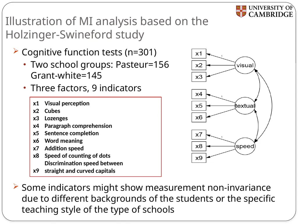
Illustration of MI analysis based on the Holzinger-Swineford study Cognitive function tests (n=301)
Two school groups: Pasteur=156 Grant-white=145
Three factors, 9 indicators Some indicators might show measurement non-invariance due to different backgrounds of the students or the specific teaching style of the type of schools<br>
Two school groups: Pasteur=156 Grant-white=145
Three factors, 9 indicators Some indicators might show measurement non-invariance due to different backgrounds of the students or the specific teaching style of the type of schools<br>
06
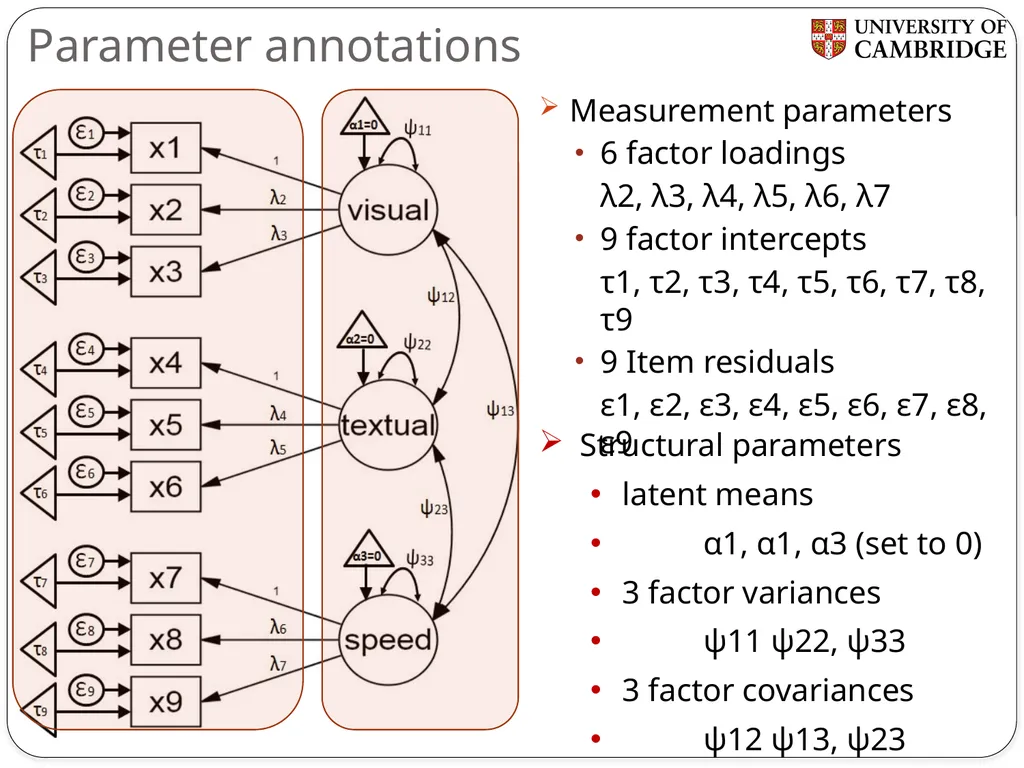
Parameter annotations Measurement parameters
6 factor loadings
λ2, λ3, λ4, λ5, λ6, λ7
9 factor intercepts
τ1, τ2, τ3, τ4, τ5, τ6, τ7, τ8, τ9
9 Item residuals
ε1, ε2, ε3, ε4, ε5, ε6, ε7, ε8, ε9 Structural parameters
latent means
α1, α1, α3 (set to 0)
3 factor variances
ψ11 ψ22, ψ33
3 factor covariances
ψ12 ψ13, ψ23<br>
6 factor loadings
λ2, λ3, λ4, λ5, λ6, λ7
9 factor intercepts
τ1, τ2, τ3, τ4, τ5, τ6, τ7, τ8, τ9
9 Item residuals
ε1, ε2, ε3, ε4, ε5, ε6, ε7, ε8, ε9 Structural parameters
latent means
α1, α1, α3 (set to 0)
3 factor variances
ψ11 ψ22, ψ33
3 factor covariances
ψ12 ψ13, ψ23<br>
07
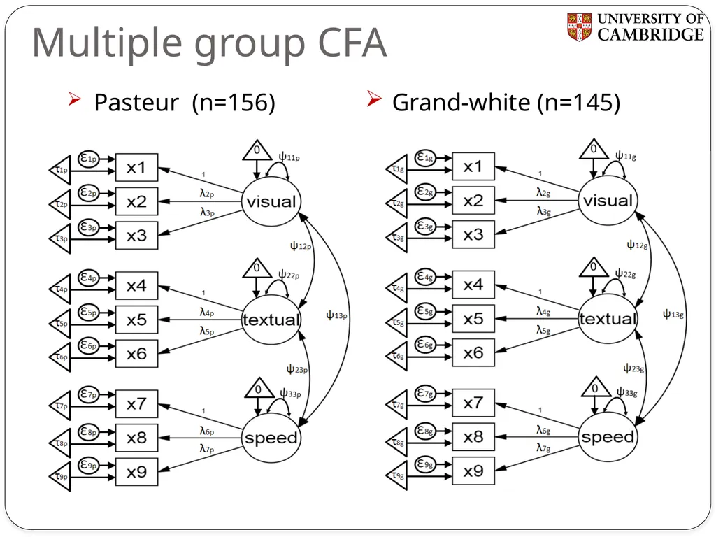
Multiple group CFA Pasteur (n=156) Grand-white (n=145)<br>
08
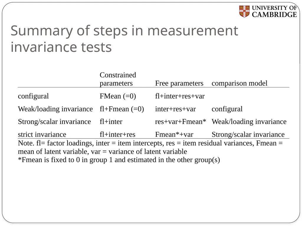
Summary of steps in measurement invariance tests<br>
09
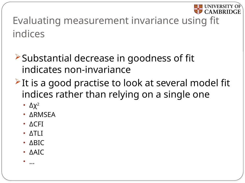
Evaluating measurement invariance using fit indices Substantial decrease in goodness of fit indicates non-invariance
It is a good practise to look at several model fit indices rather than relying on a single one
Δχ2
ΔRMSEA
ΔCFI
ΔTLI
ΔBIC
ΔAIC
…<br>
It is a good practise to look at several model fit indices rather than relying on a single one
Δχ2
ΔRMSEA
ΔCFI
ΔTLI
ΔBIC
ΔAIC
…<br>
10
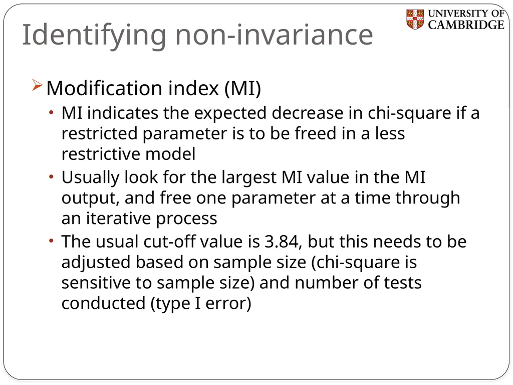
Identifying non-invariance Modification index (MI)
MI indicates the expected decrease in chi-square if a restricted parameter is to be freed in a less restrictive model
Usually look for the largest MI value in the MI output, and free one parameter at a time through an iterative process
The usual cut-off value is 3.84, but this needs to be adjusted based on sample size (chi-square is sensitive to sample size) and number of tests conducted (type I error)<br>
MI indicates the expected decrease in chi-square if a restricted parameter is to be freed in a less restrictive model
Usually look for the largest MI value in the MI output, and free one parameter at a time through an iterative process
The usual cut-off value is 3.84, but this needs to be adjusted based on sample size (chi-square is sensitive to sample size) and number of tests conducted (type I error)<br>
11
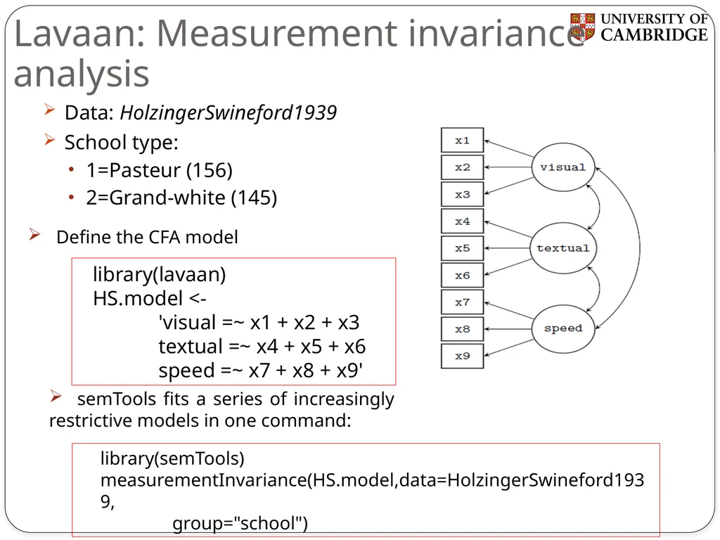
Lavaan: Measurement invariance analysis Data: HolzingerSwineford1939
School type:
1=Pasteur (156)
2=Grand-white (145) library(lavaan)
HS.model <-
'visual =~ x1 + x2 + x3
textual =~ x4 + x5 + x6
speed =~ x7 + x8 + x9' library(semTools)
measurementInvariance(HS.model,data=HolzingerSwineford1939,
group="school") semTools fits a series of increasingly restrictive models in one command: Define the CFA model<br>
School type:
1=Pasteur (156)
2=Grand-white (145) library(lavaan)
HS.model <-
'visual =~ x1 + x2 + x3
textual =~ x4 + x5 + x6
speed =~ x7 + x8 + x9' library(semTools)
measurementInvariance(HS.model,data=HolzingerSwineford1939,
group="school") semTools fits a series of increasingly restrictive models in one command: Define the CFA model<br>
12
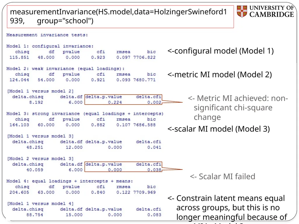
measurementInvariance(HS.model,data=HolzingerSwineford1939, group="school") <-configural model (Model 1)
<-metric MI model (Model 2)
<- Metric MI achieved: non- significant chi-square change
<-scalar MI model (Model 3)
<- Scalar MI failed
<- Constrain latent means equal across groups, but this is no longer meaningful because of non-MI in Model 3.<br>
<-metric MI model (Model 2)
<- Metric MI achieved: non- significant chi-square change
<-scalar MI model (Model 3)
<- Scalar MI failed
<- Constrain latent means equal across groups, but this is no longer meaningful because of non-MI in Model 3.<br>
13
Measurement invariance:
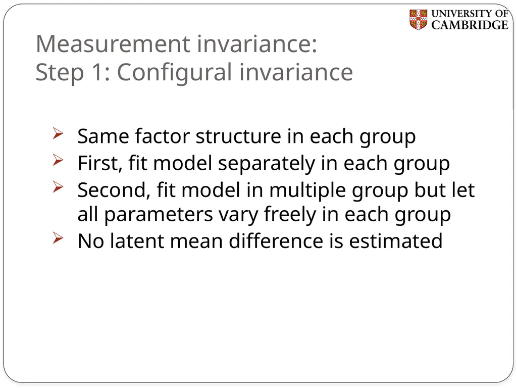
Step 1: Configural invariance Same factor structure in each group
First, fit model separately in each group
Second, fit model in multiple group but let all parameters vary freely in each group
No latent mean difference is estimated<br>
First, fit model separately in each group
Second, fit model in multiple group but let all parameters vary freely in each group
No latent mean difference is estimated<br>
14
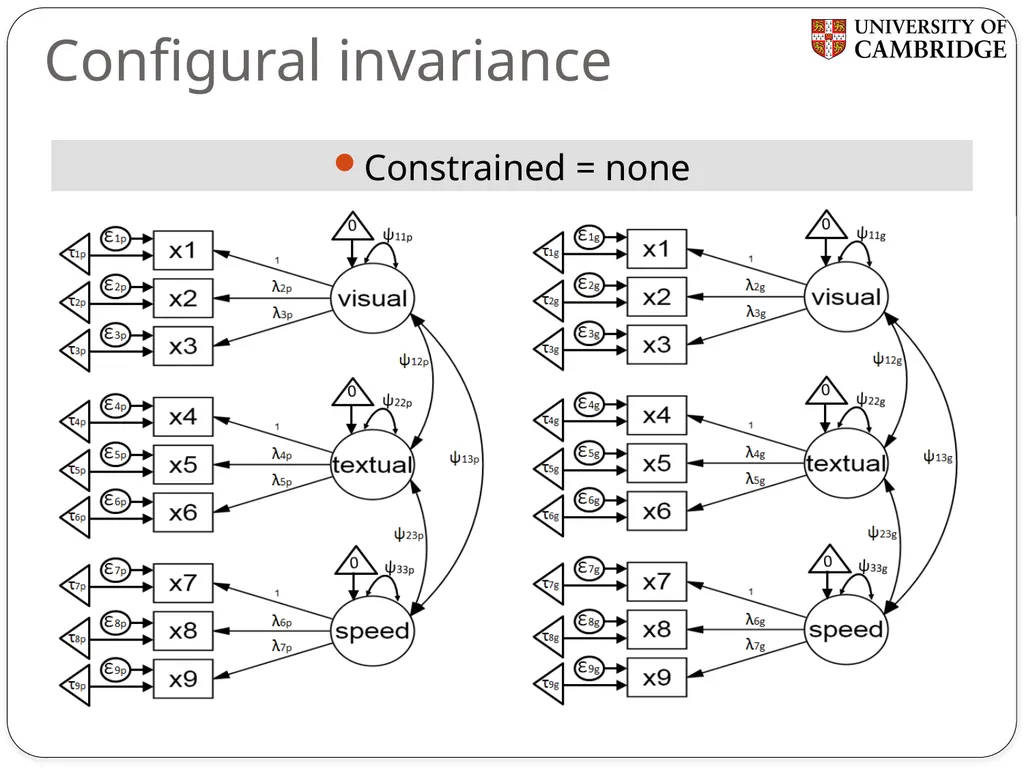
Configural invariance Constrained = none<br>
15
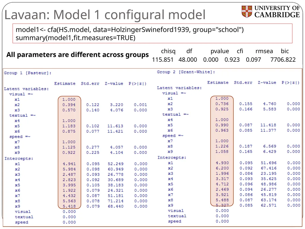
Lavaan: Model 1 configural model chisq df pvalue cfi rmsea bic
115.851 48.000 0.000 0.923 0.097 7706.822 model1<- cfa(HS.model, data=HolzingerSwineford1939, group="school")
summary(model1,fit.measures=TRUE) All parameters are different across groups<br>
115.851 48.000 0.000 0.923 0.097 7706.822 model1<- cfa(HS.model, data=HolzingerSwineford1939, group="school")
summary(model1,fit.measures=TRUE) All parameters are different across groups<br>
16
Measurement invariance:
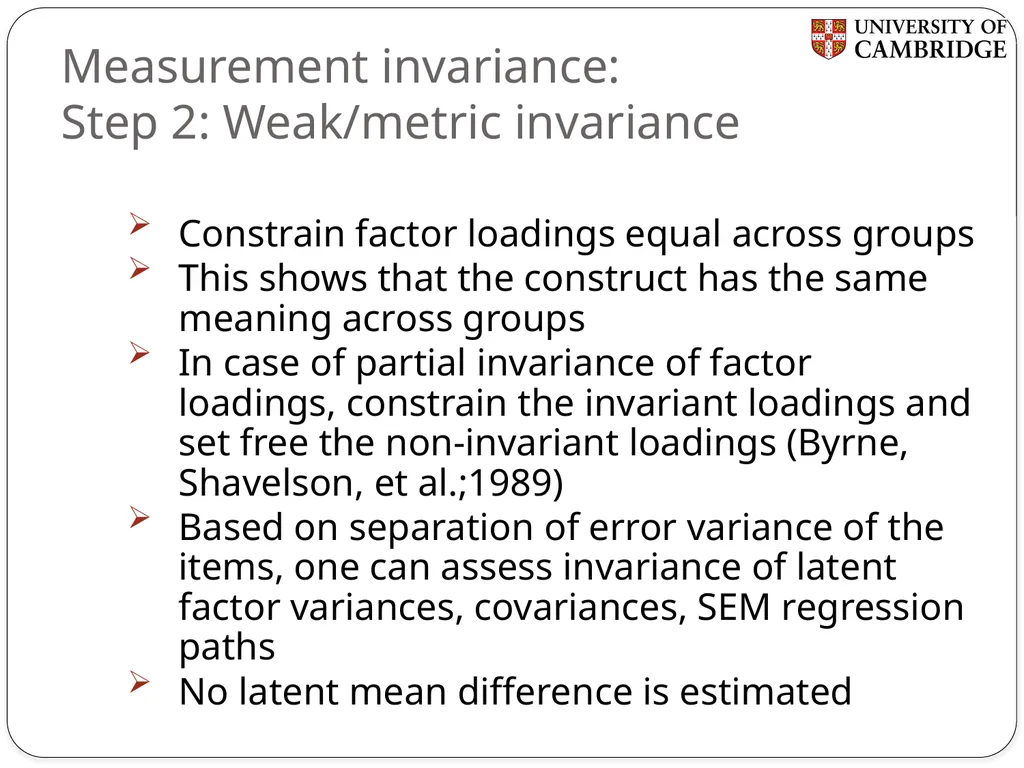
Step 2: Weak/metric invariance Constrain factor loadings equal across groups
This shows that the construct has the same meaning across groups
In case of partial invariance of factor loadings, constrain the invariant loadings and set free the non-invariant loadings (Byrne, Shavelson, et al.;1989)
Based on separation of error variance of the items, one can assess invariance of latent factor variances, covariances, SEM regression paths
No latent mean difference is estimated<br>
This shows that the construct has the same meaning across groups
In case of partial invariance of factor loadings, constrain the invariant loadings and set free the non-invariant loadings (Byrne, Shavelson, et al.;1989)
Based on separation of error variance of the items, one can assess invariance of latent factor variances, covariances, SEM regression paths
No latent mean difference is estimated<br>
17
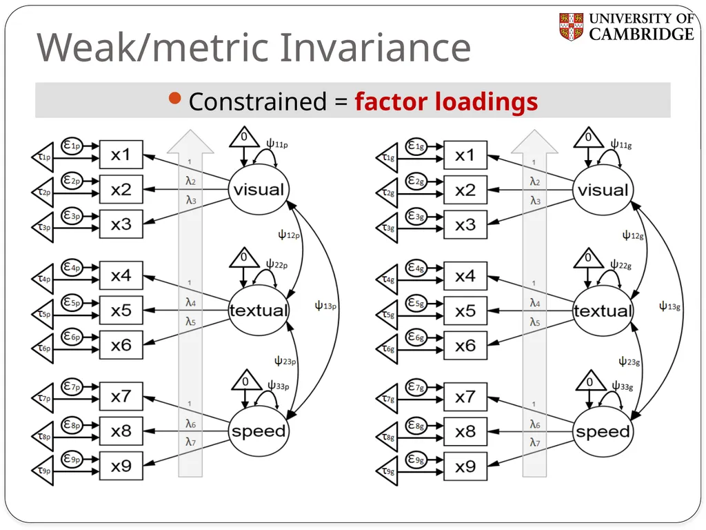
Weak/metric Invariance Constrained = factor loadings<br>
18
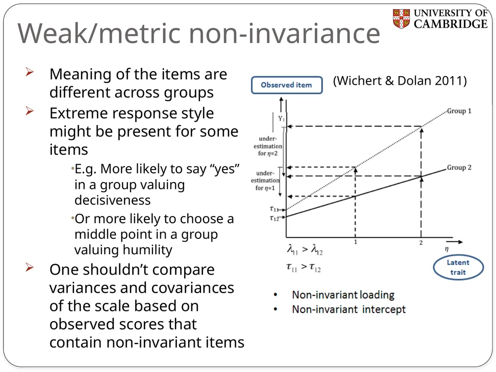
Weak/metric non-invariance Meaning of the items are different across groups
Extreme response style might be present for some items
E.g. More likely to say “yes” in a group valuing decisiveness
Or more likely to choose a middle point in a group valuing humility
One shouldn’t compare variances and covariances of the scale based on observed scores that contain non-invariant items (Wichert & Dolan 2011)<br>
Extreme response style might be present for some items
E.g. More likely to say “yes” in a group valuing decisiveness
Or more likely to choose a middle point in a group valuing humility
One shouldn’t compare variances and covariances of the scale based on observed scores that contain non-invariant items (Wichert & Dolan 2011)<br>
19
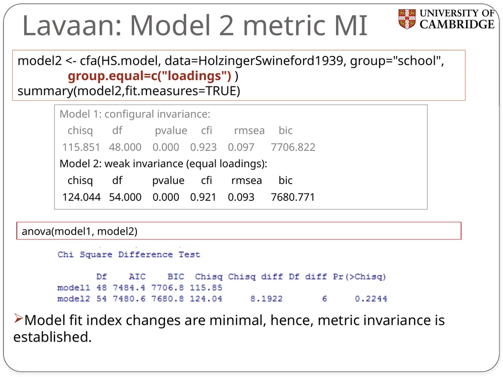
Lavaan: Model 2 metric MI Model 1: configural invariance:
chisq df pvalue cfi rmsea bic
115.851 48.000 0.000 0.923 0.097 7706.822
Model 2: weak invariance (equal loadings):
chisq df pvalue cfi rmsea bic
124.044 54.000 0.000 0.921 0.093 7680.771 anova(model1, model2) Model fit index changes are minimal, hence, metric invariance is established. model2 <- cfa(HS.model, data=HolzingerSwineford1939, group="school", group.equal=c("loadings") )
summary(model2,fit.measures=TRUE)<br>
chisq df pvalue cfi rmsea bic
115.851 48.000 0.000 0.923 0.097 7706.822
Model 2: weak invariance (equal loadings):
chisq df pvalue cfi rmsea bic
124.044 54.000 0.000 0.921 0.093 7680.771 anova(model1, model2) Model fit index changes are minimal, hence, metric invariance is established. model2 <- cfa(HS.model, data=HolzingerSwineford1939, group="school", group.equal=c("loadings") )
summary(model2,fit.measures=TRUE)<br>
20
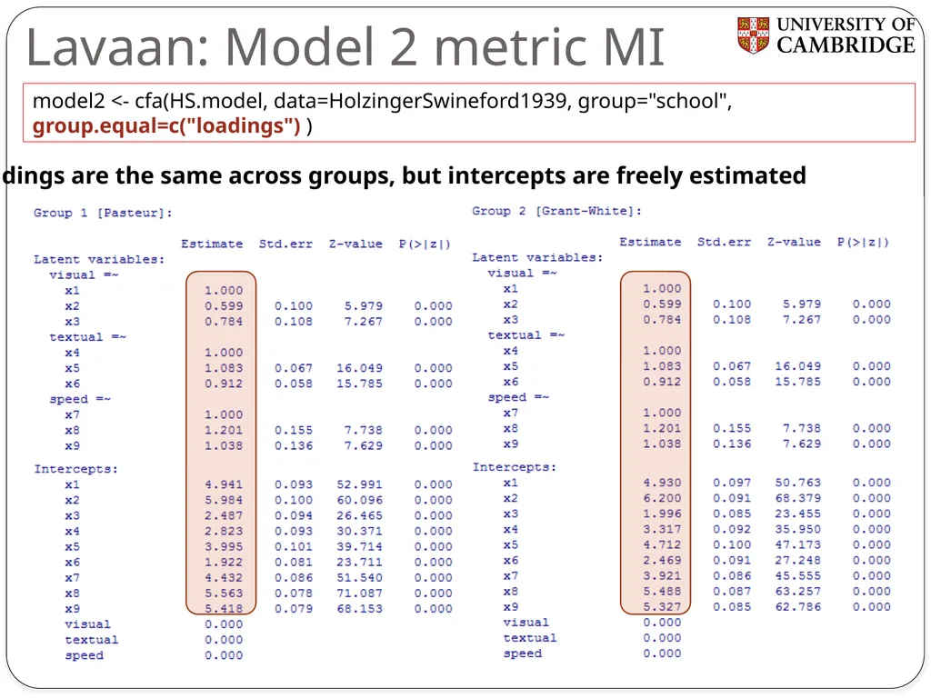
Lavaan: Model 2 metric MI model2 <- cfa(HS.model, data=HolzingerSwineford1939, group="school", group.equal=c("loadings") ) Loadings are the same across groups, but intercepts are freely estimated<br>
21
Measurement invariance:
Step 3: Strong/scalar invariance Constrain item intercepts equal across groups
Constrain factor loadings
This is important for assessing mean difference of the latent variable across groups
In case of partial invariance of item intercepts, constrain the invariant intercepts and set free the non-invariant intercepts (Byrne, Shavelson, et al.;1989)
Latent mean difference is estimated<br>
Constrain factor loadings
This is important for assessing mean difference of the latent variable across groups
In case of partial invariance of item intercepts, constrain the invariant intercepts and set free the non-invariant intercepts (Byrne, Shavelson, et al.;1989)
Latent mean difference is estimated<br>
22
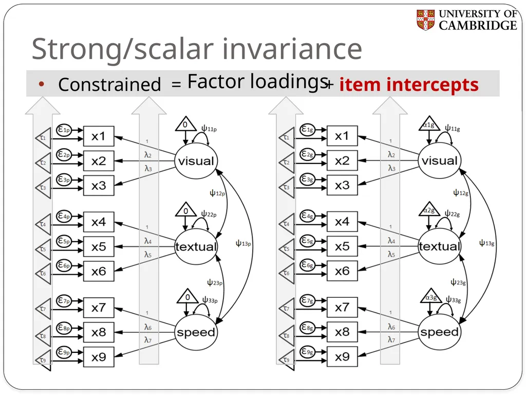
Strong/scalar invariance Factor loadings Constrained = + item intercepts<br>
23
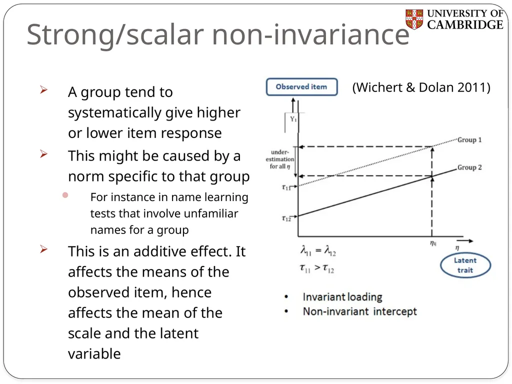
Strong/scalar non-invariance A group tend to systematically give higher or lower item response
This might be caused by a norm specific to that group
For instance in name learning tests that involve unfamiliar names for a group
This is an additive effect. It affects the means of the observed item, hence affects the mean of the scale and the latent variable (Wichert & Dolan 2011)<br>
This might be caused by a norm specific to that group
For instance in name learning tests that involve unfamiliar names for a group
This is an additive effect. It affects the means of the observed item, hence affects the mean of the scale and the latent variable (Wichert & Dolan 2011)<br>
24
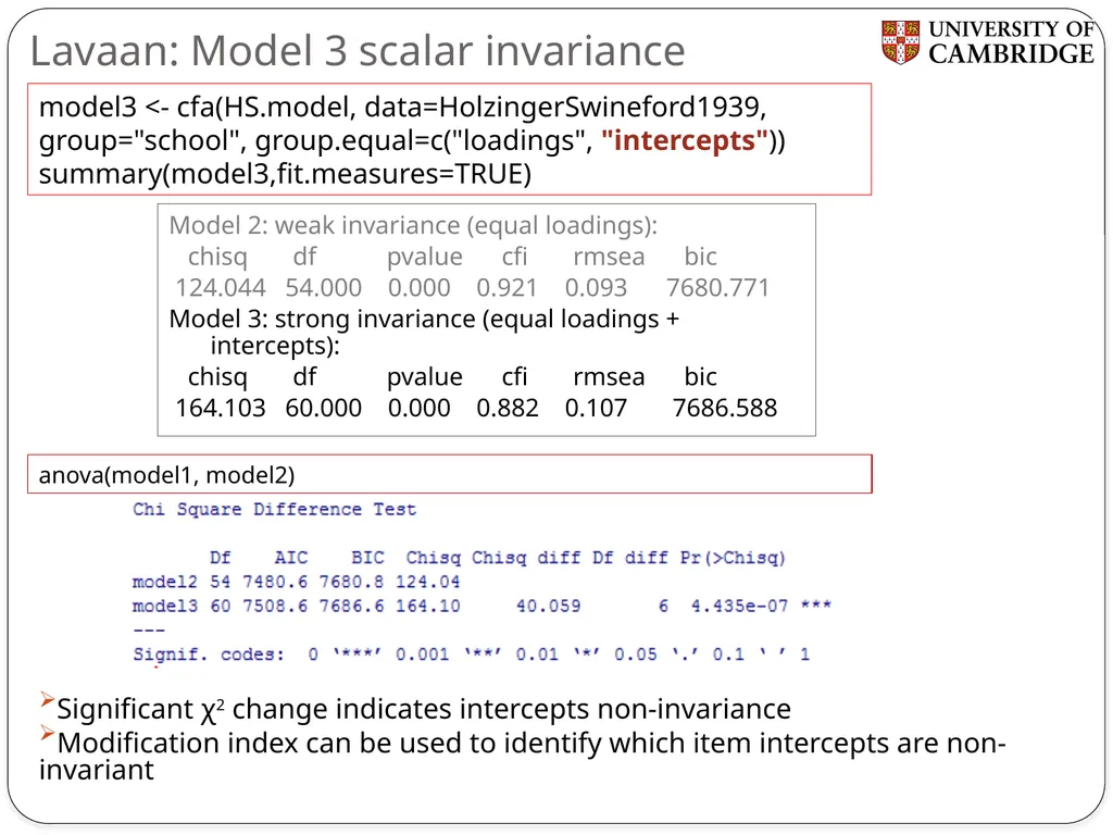
Lavaan: Model 3 scalar invariance Significant χ2 change indicates intercepts non-invariance
Modification index can be used to identify which item intercepts are non-invariant Model 2: weak invariance (equal loadings):
chisq df pvalue cfi rmsea bic
124.044 54.000 0.000 0.921 0.093 7680.771
Model 3: strong invariance (equal loadings + intercepts):
chisq df pvalue cfi rmsea bic
164.103 60.000 0.000 0.882 0.107 7686.588 model3 <- cfa(HS.model, data=HolzingerSwineford1939, group="school", group.equal=c("loadings", "intercepts"))
summary(model3,fit.measures=TRUE) anova(model1, model2)<br>
Modification index can be used to identify which item intercepts are non-invariant Model 2: weak invariance (equal loadings):
chisq df pvalue cfi rmsea bic
124.044 54.000 0.000 0.921 0.093 7680.771
Model 3: strong invariance (equal loadings + intercepts):
chisq df pvalue cfi rmsea bic
164.103 60.000 0.000 0.882 0.107 7686.588 model3 <- cfa(HS.model, data=HolzingerSwineford1939, group="school", group.equal=c("loadings", "intercepts"))
summary(model3,fit.measures=TRUE) anova(model1, model2)<br>
25
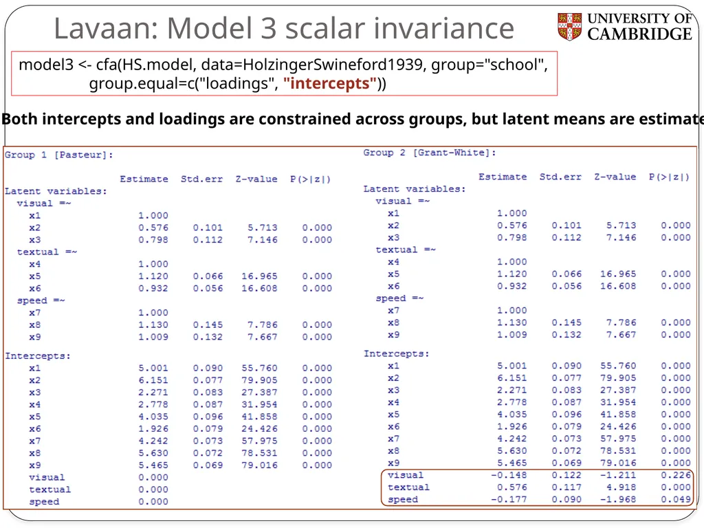
model3 <- cfa(HS.model, data=HolzingerSwineford1939, group="school", group.equal=c("loadings", "intercepts")) Lavaan: Model 3 scalar invariance Both intercepts and loadings are constrained across groups, but latent means are estimated<br>
26
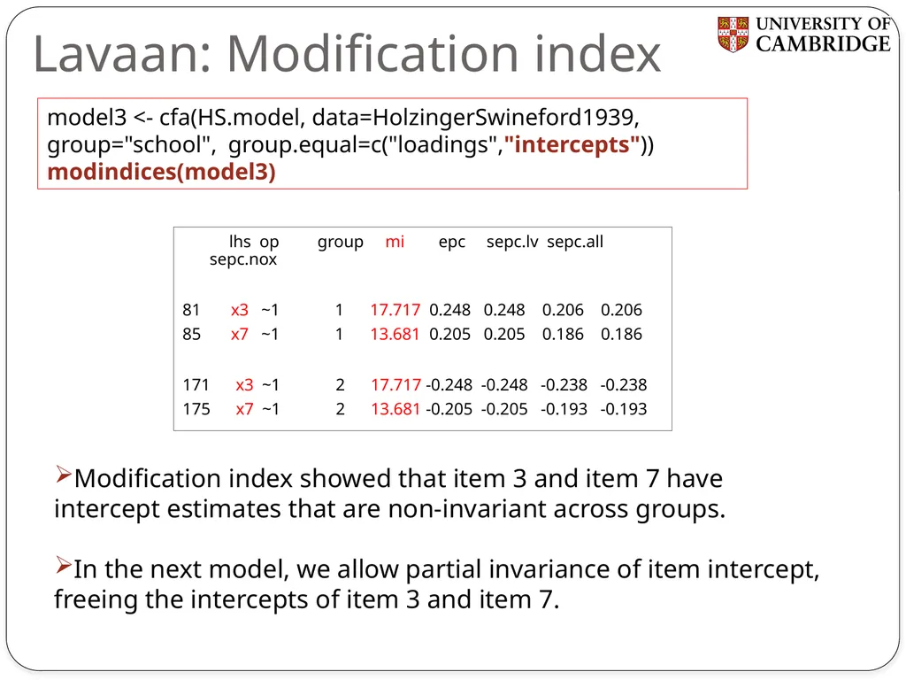
Lavaan: Modification index lhs op group mi epc sepc.lv sepc.all sepc.nox
81 x3 ~1 1 17.717 0.248 0.248 0.206 0.206
85 x7 ~1 1 13.681 0.205 0.205 0.186 0.186
171 x3 ~1 2 17.717 -0.248 -0.248 -0.238 -0.238
175 x7 ~1 2 13.681 -0.205 -0.205 -0.193 -0.193 model3 <- cfa(HS.model, data=HolzingerSwineford1939, group="school", group.equal=c("loadings","intercepts"))
modindices(model3) Modification index showed that item 3 and item 7 have intercept estimates that are non-invariant across groups.
In the next model, we allow partial invariance of item intercept, freeing the intercepts of item 3 and item 7.<br>
81 x3 ~1 1 17.717 0.248 0.248 0.206 0.206
85 x7 ~1 1 13.681 0.205 0.205 0.186 0.186
171 x3 ~1 2 17.717 -0.248 -0.248 -0.238 -0.238
175 x7 ~1 2 13.681 -0.205 -0.205 -0.193 -0.193 model3 <- cfa(HS.model, data=HolzingerSwineford1939, group="school", group.equal=c("loadings","intercepts"))
modindices(model3) Modification index showed that item 3 and item 7 have intercept estimates that are non-invariant across groups.
In the next model, we allow partial invariance of item intercept, freeing the intercepts of item 3 and item 7.<br>
27
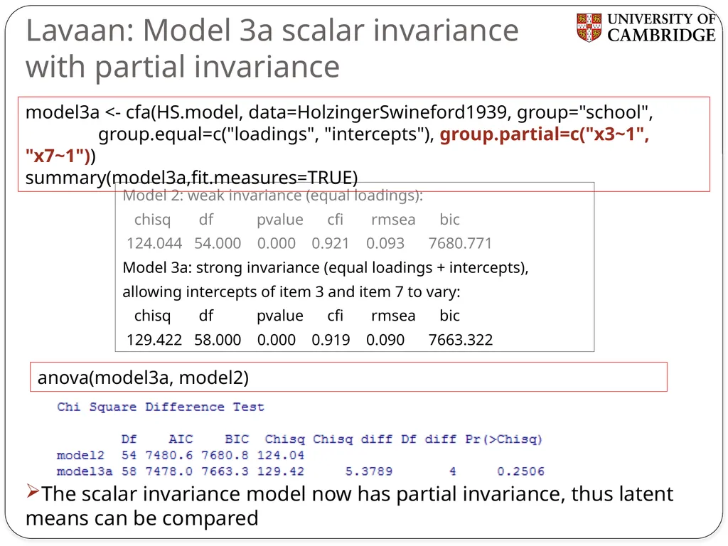
Lavaan: Model 3a scalar invariance with partial invariance Model 2: weak invariance (equal loadings):
chisq df pvalue cfi rmsea bic
124.044 54.000 0.000 0.921 0.093 7680.771
Model 3a: strong invariance (equal loadings + intercepts),
allowing intercepts of item 3 and item 7 to vary:
chisq df pvalue cfi rmsea bic
129.422 58.000 0.000 0.919 0.090 7663.322 model3a <- cfa(HS.model, data=HolzingerSwineford1939, group="school",
group.equal=c("loadings", "intercepts"), group.partial=c("x3~1", "x7~1"))
summary(model3a,fit.measures=TRUE) The scalar invariance model now has partial invariance, thus latent means can be compared anova(model3a, model2)<br>
chisq df pvalue cfi rmsea bic
124.044 54.000 0.000 0.921 0.093 7680.771
Model 3a: strong invariance (equal loadings + intercepts),
allowing intercepts of item 3 and item 7 to vary:
chisq df pvalue cfi rmsea bic
129.422 58.000 0.000 0.919 0.090 7663.322 model3a <- cfa(HS.model, data=HolzingerSwineford1939, group="school",
group.equal=c("loadings", "intercepts"), group.partial=c("x3~1", "x7~1"))
summary(model3a,fit.measures=TRUE) The scalar invariance model now has partial invariance, thus latent means can be compared anova(model3a, model2)<br>
28
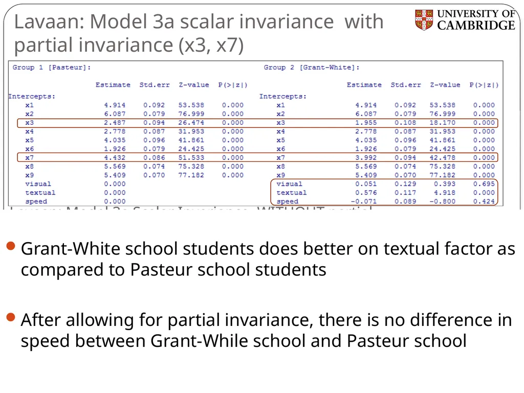
Lavaan: Model 3a scalar invariance with partial invariance (x3, x7) Lavaan: Model 3a Scalar Invariance WITHOUT partial invariance Grant-White school students does better on textual factor as compared to Pasteur school students
After allowing for partial invariance, there is no difference in speed between Grant-While school and Pasteur school<br>
After allowing for partial invariance, there is no difference in speed between Grant-While school and Pasteur school<br>
29
Measurement invariance:
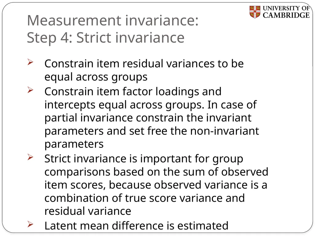
Step 4: Strict invariance Constrain item residual variances to be equal across groups
Constrain item factor loadings and intercepts equal across groups. In case of partial invariance constrain the invariant parameters and set free the non-invariant parameters
Strict invariance is important for group comparisons based on the sum of observed item scores, because observed variance is a combination of true score variance and residual variance
Latent mean difference is estimated<br>
Constrain item factor loadings and intercepts equal across groups. In case of partial invariance constrain the invariant parameters and set free the non-invariant parameters
Strict invariance is important for group comparisons based on the sum of observed item scores, because observed variance is a combination of true score variance and residual variance
Latent mean difference is estimated<br>
30
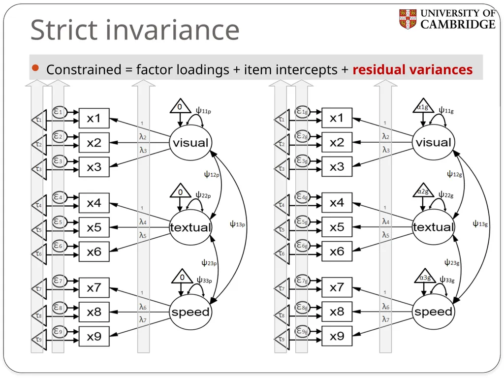
Strict invariance Constrained = factor loadings + item intercepts + residual variances<br>
31
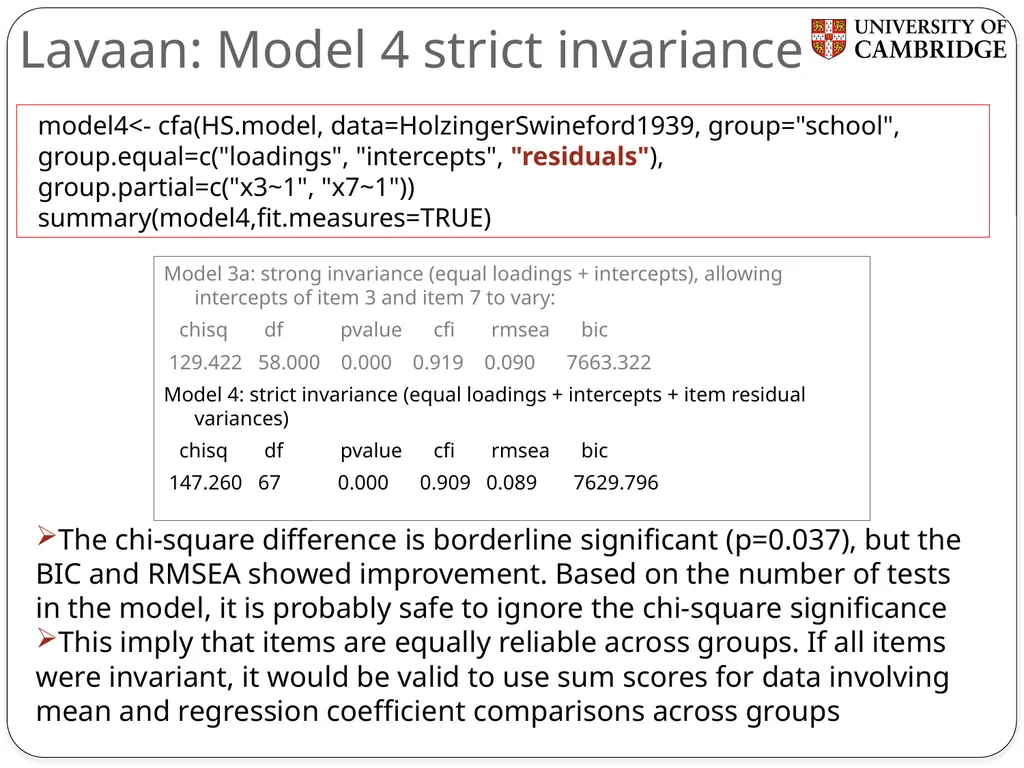
Lavaan: Model 4 strict invariance Model 3a: strong invariance (equal loadings + intercepts), allowing intercepts of item 3 and item 7 to vary:
chisq df pvalue cfi rmsea bic
129.422 58.000 0.000 0.919 0.090 7663.322
Model 4: strict invariance (equal loadings + intercepts + item residual variances)
chisq df pvalue cfi rmsea bic
147.260 67 0.000 0.909 0.089 7629.796 model4<- cfa(HS.model, data=HolzingerSwineford1939, group="school", group.equal=c("loadings", "intercepts", "residuals"), group.partial=c("x3~1", "x7~1"))
summary(model4,fit.measures=TRUE) The chi-square difference is borderline significant (p=0.037), but the BIC and RMSEA showed improvement. Based on the number of tests in the model, it is probably safe to ignore the chi-square significance
This imply that items are equally reliable across groups. If all items were invariant, it would be valid to use sum scores for data involving mean and regression coefficient comparisons across groups<br>
chisq df pvalue cfi rmsea bic
129.422 58.000 0.000 0.919 0.090 7663.322
Model 4: strict invariance (equal loadings + intercepts + item residual variances)
chisq df pvalue cfi rmsea bic
147.260 67 0.000 0.909 0.089 7629.796 model4<- cfa(HS.model, data=HolzingerSwineford1939, group="school", group.equal=c("loadings", "intercepts", "residuals"), group.partial=c("x3~1", "x7~1"))
summary(model4,fit.measures=TRUE) The chi-square difference is borderline significant (p=0.037), but the BIC and RMSEA showed improvement. Based on the number of tests in the model, it is probably safe to ignore the chi-square significance
This imply that items are equally reliable across groups. If all items were invariant, it would be valid to use sum scores for data involving mean and regression coefficient comparisons across groups<br>
32
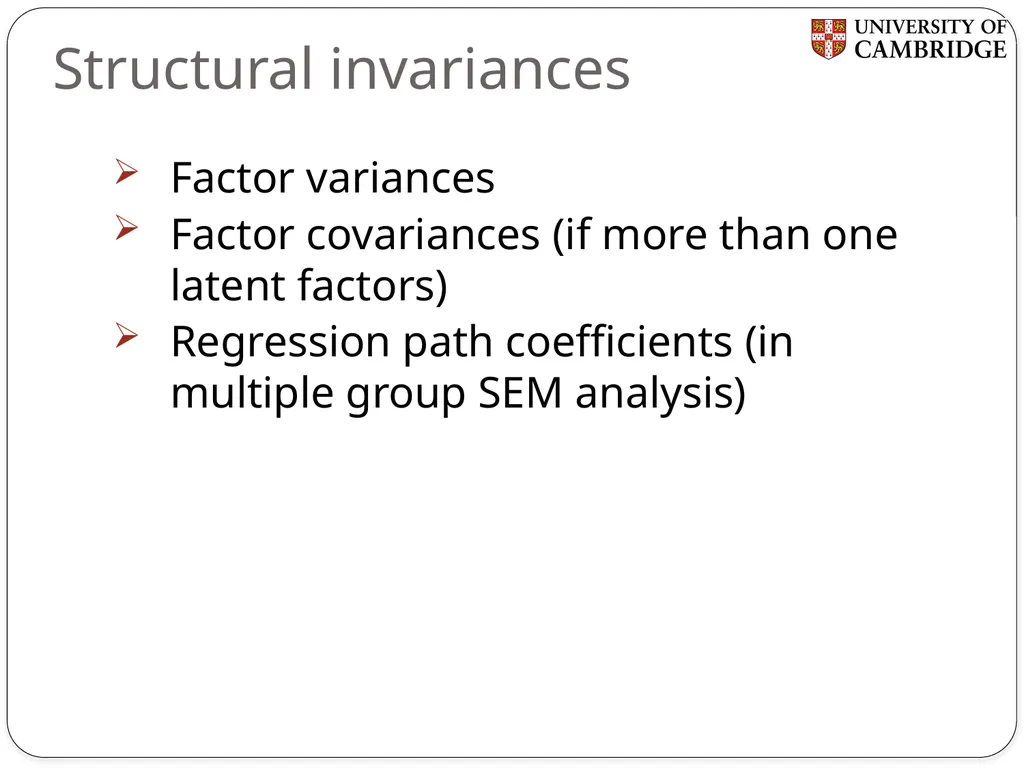
Structural invariances Factor variances
Factor covariances (if more than one latent factors)
Regression path coefficients (in multiple group SEM analysis)<br>
Factor covariances (if more than one latent factors)
Regression path coefficients (in multiple group SEM analysis)<br>
33
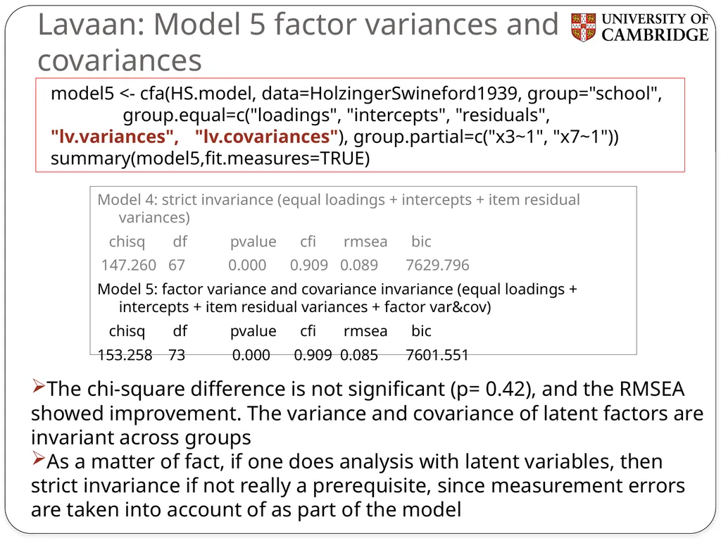
Lavaan: Model 5 factor variances and covariances Model 4: strict invariance (equal loadings + intercepts + item residual variances)
chisq df pvalue cfi rmsea bic
147.260 67 0.000 0.909 0.089 7629.796
Model 5: factor variance and covariance invariance (equal loadings + intercepts + item residual variances + factor var&cov)
chisq df pvalue cfi rmsea bic
153.258 73 0.000 0.909 0.085 7601.551 model5 <- cfa(HS.model, data=HolzingerSwineford1939, group="school",
group.equal=c("loadings", "intercepts", "residuals", "lv.variances", "lv.covariances"), group.partial=c("x3~1", "x7~1"))
summary(model5,fit.measures=TRUE) The chi-square difference is not significant (p= 0.42), and the RMSEA showed improvement. The variance and covariance of latent factors are invariant across groups
As a matter of fact, if one does analysis with latent variables, then strict invariance if not really a prerequisite, since measurement errors are taken into account of as part of the model<br>
chisq df pvalue cfi rmsea bic
147.260 67 0.000 0.909 0.089 7629.796
Model 5: factor variance and covariance invariance (equal loadings + intercepts + item residual variances + factor var&cov)
chisq df pvalue cfi rmsea bic
153.258 73 0.000 0.909 0.085 7601.551 model5 <- cfa(HS.model, data=HolzingerSwineford1939, group="school",
group.equal=c("loadings", "intercepts", "residuals", "lv.variances", "lv.covariances"), group.partial=c("x3~1", "x7~1"))
summary(model5,fit.measures=TRUE) The chi-square difference is not significant (p= 0.42), and the RMSEA showed improvement. The variance and covariance of latent factors are invariant across groups
As a matter of fact, if one does analysis with latent variables, then strict invariance if not really a prerequisite, since measurement errors are taken into account of as part of the model<br>
34
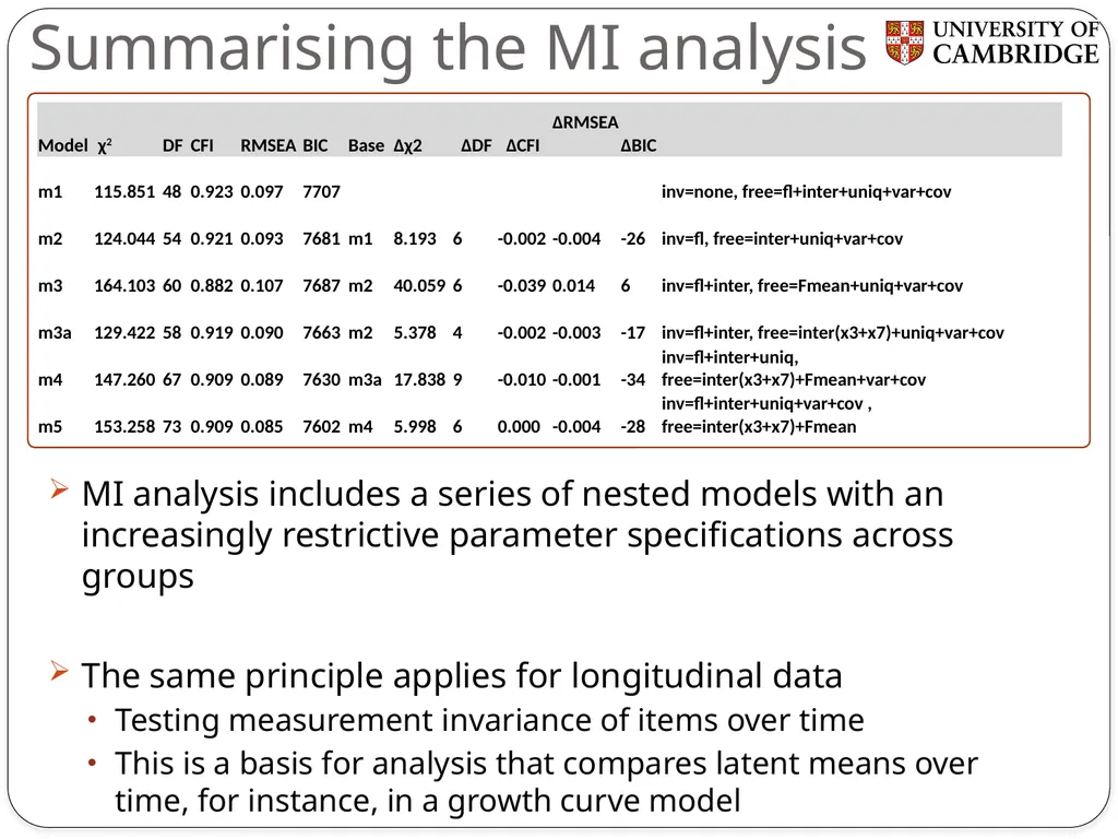
Summarising the MI analysis MI analysis includes a series of nested models with an increasingly restrictive parameter specifications across groups
The same principle applies for longitudinal data
Testing measurement invariance of items over time
This is a basis for analysis that compares latent means over time, for instance, in a growth curve model<br>
The same principle applies for longitudinal data
Testing measurement invariance of items over time
This is a basis for analysis that compares latent means over time, for instance, in a growth curve model<br>
35
Measurement invariance
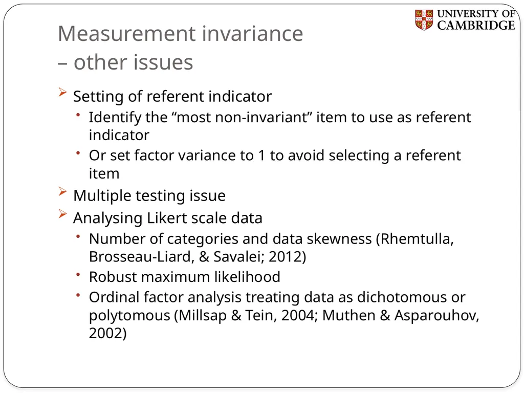
– other issues Setting of referent indicator
Identify the “most non-invariant” item to use as referent indicator
Or set factor variance to 1 to avoid selecting a referent item
Multiple testing issue
Analysing Likert scale data
Number of categories and data skewness (Rhemtulla, Brosseau-Liard, & Savalei; 2012)
Robust maximum likelihood
Ordinal factor analysis treating data as dichotomous or polytomous (Millsap & Tein, 2004; Muthen & Asparouhov, 2002)<br>
Identify the “most non-invariant” item to use as referent indicator
Or set factor variance to 1 to avoid selecting a referent item
Multiple testing issue
Analysing Likert scale data
Number of categories and data skewness (Rhemtulla, Brosseau-Liard, & Savalei; 2012)
Robust maximum likelihood
Ordinal factor analysis treating data as dichotomous or polytomous (Millsap & Tein, 2004; Muthen & Asparouhov, 2002)<br>
36
Some references Sass, D. A. (2011). "Testing Measurement Invariance and Comparing Latent Factor Means Within a Confirmatory Factor Analysis Framework." Journal of Psychoeducational Assessment 29(4): 347-363.
Wicherts, J. M. and C. V. Dolan (2010). "Measurement invariance in confirmatory factor analysis: An illustration using IQ test performance of minorities." Educational Measurement: Issues and Practice 29(3): 39-47.
Gregorich, S. E. (2006). "Do self-report instruments allow meaningful comparisons across diverse population groups? Testing measurement invariance using the confirmatory factor analysis framework." Medical Care 44(11 Suppl 3): S78.
Byrne, B. M., R. J. Shavelson, et al. (1989). "Testing for the equivalence of factor covariance and mean structures: The issue of partial measurement invariance." Psychological bulletin 105(3): 456-466.
Millsap, R. E. and J. Yun-Tein (2004). "Assessing factorial invariance in ordered-categorical measures." Multivariate Behavioral Research 39(3): 479-515.
Meredith, W. (1993). "Measurement invariance, factor analysis and factorial invariance." Psychometrika 58(4): 525-543.
Rhemtulla, M., Brosseau-Liard, P. É., & Savalei, V. (2012). When can categorical variables be treated as continuous? A comparison of robust continuous and categorical SEM estimation methods under suboptimal conditions. Psychological Methods, 17(3), 354-373. doi: 10.1037/a0029315<br>
Wicherts, J. M. and C. V. Dolan (2010). "Measurement invariance in confirmatory factor analysis: An illustration using IQ test performance of minorities." Educational Measurement: Issues and Practice 29(3): 39-47.
Gregorich, S. E. (2006). "Do self-report instruments allow meaningful comparisons across diverse population groups? Testing measurement invariance using the confirmatory factor analysis framework." Medical Care 44(11 Suppl 3): S78.
Byrne, B. M., R. J. Shavelson, et al. (1989). "Testing for the equivalence of factor covariance and mean structures: The issue of partial measurement invariance." Psychological bulletin 105(3): 456-466.
Millsap, R. E. and J. Yun-Tein (2004). "Assessing factorial invariance in ordered-categorical measures." Multivariate Behavioral Research 39(3): 479-515.
Meredith, W. (1993). "Measurement invariance, factor analysis and factorial invariance." Psychometrika 58(4): 525-543.
Rhemtulla, M., Brosseau-Liard, P. É., & Savalei, V. (2012). When can categorical variables be treated as continuous? A comparison of robust continuous and categorical SEM estimation methods under suboptimal conditions. Psychological Methods, 17(3), 354-373. doi: 10.1037/a0029315<br>
37
Acknowledgement:
Dr. Adam Wagner provided thoughtful comments on earlier drafts<br>