Multipole Analysis of Electromagnetic Scattering
Description: Multipole Analysis of Electromagnetic Scattering COMSOL Multipole Expansion The field scattered by a particle, regardless of the particles geometrical shape or composition, can always be expressed through the multipole expansion. The
Related Topics
Download Presentation
"Multipole Analysis of Electromagnetic Scattering" is the property of its rightful owner. Permission is granted to download and print the materials on this website for personal, non-commercial use only, and to display it on your personal computer provided you do not modify the materials and that you retain all copyright notices contained in the materials. By downloading content from our website, you accept the terms of this agreement.
Presentation Transcript
slide1. Multipole Analysis of Electromagnetic Scattering COMSOL<br>
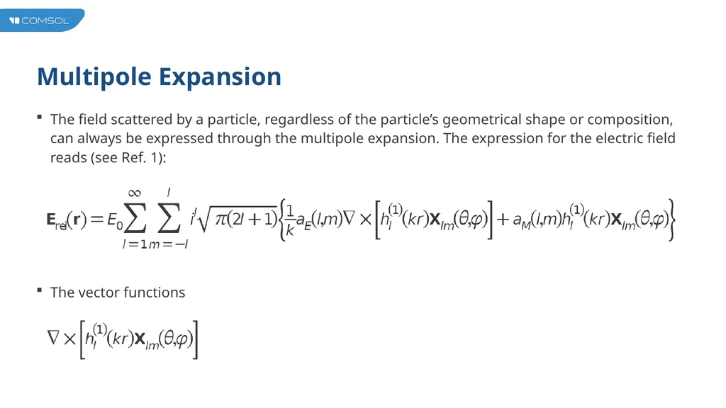
slide2. Multipole Expansion The field scattered by a particle, regardless of the particle’s geometrical shape or composition, can always be expressed through the multipole expansion. The expression for the electric field reads (see Ref. 1): The vector functions<br>
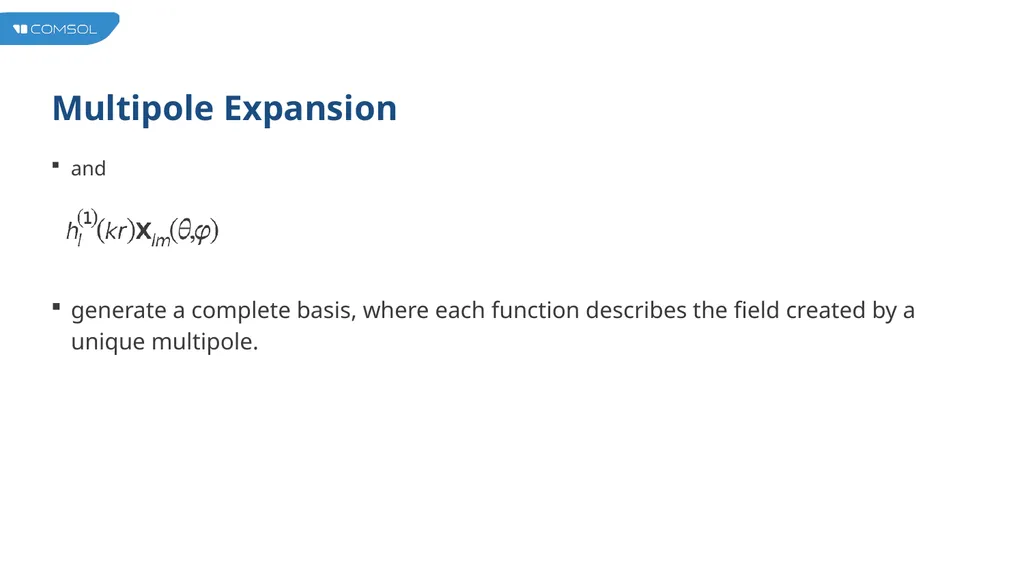
slide3. Multipole Expansion and generate a complete basis, where each function describes the field created by a unique multipole.<br>
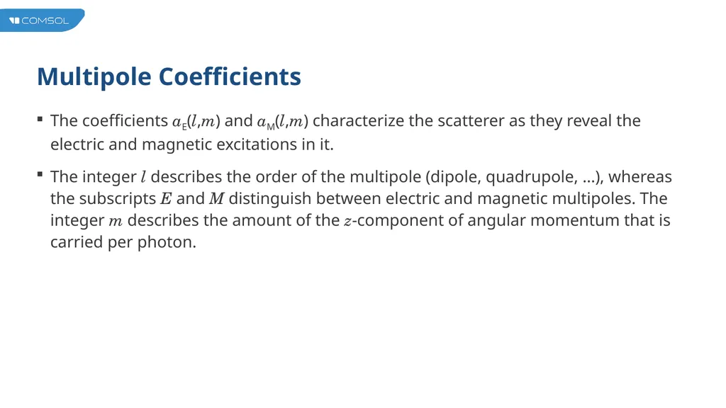
slide4. Multipole Coefficients The coefficients aE(l,m) and aM(l,m) characterize the scatterer as they reveal the electric and magnetic excitations in it.
The integer l describes the order of the multipole (dipole, quadrupole, …), whereas the subscripts E and M distinguish between electric and magnetic multipoles. The integer m describes the amount of the z-component of angular momentum that is carried per photon.<br>
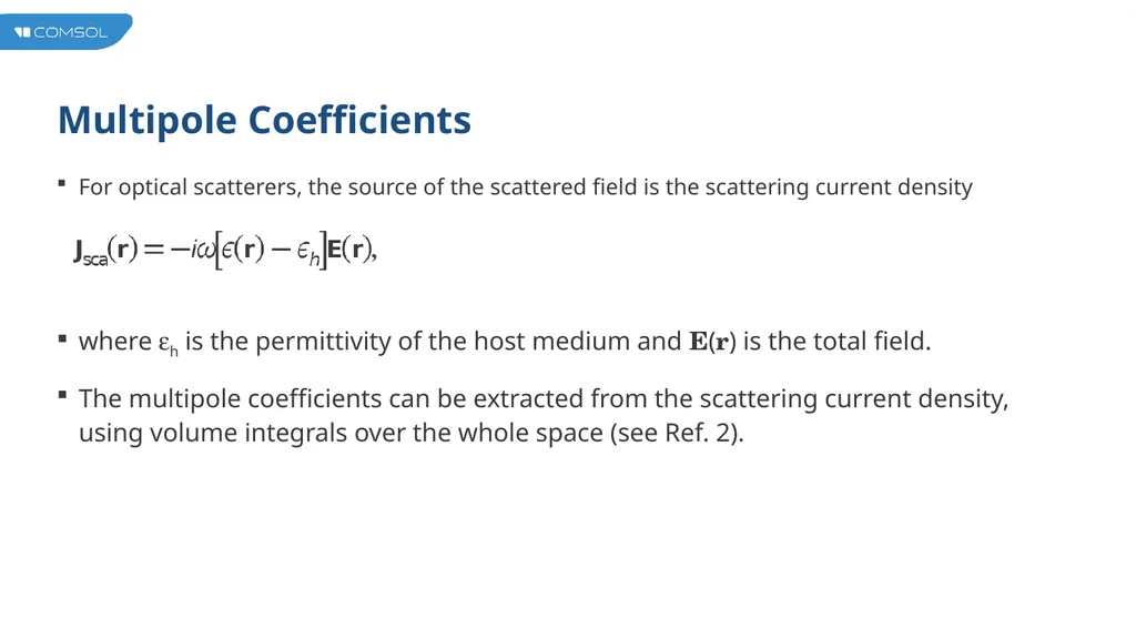
slide5. Multipole Coefficients For optical scatterers, the source of the scattered field is the scattering current density where eh is the permittivity of the host medium and E(r) is the total field.
The multipole coefficients can be extracted from the scattering current density, using volume integrals over the whole space (see Ref. 2).<br>
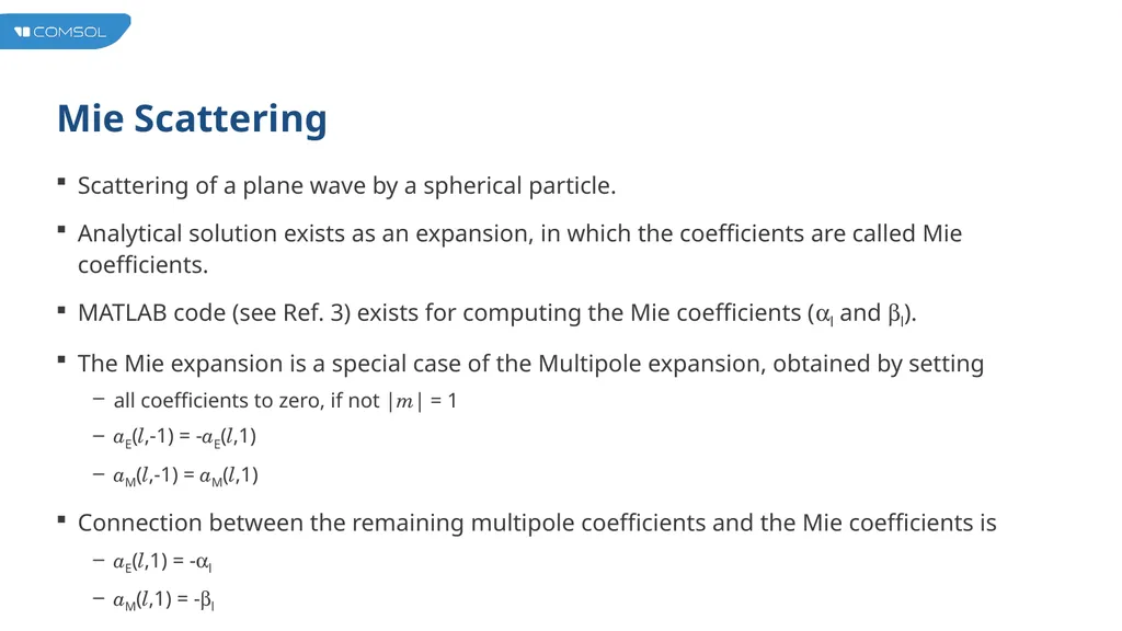
slide6. Mie Scattering Scattering of a plane wave by a spherical particle.
Analytical solution exists as an expansion, in which the coefficients are called Mie coefficients.
MATLAB code (see Ref. 3) exists for computing the Mie coefficients (al and bl).
The Mie expansion is a special case of the Multipole expansion, obtained by setting
all coefficients to zero, if not |m| = 1
aE(l,-1) = -aE(l,1)
aM(l,-1) = aM(l,1)
Connection between the remaining multipole coefficients and the Mie coefficients is
aE(l,1) = -al
aM(l,1) = -bl<br>
slide7. COMSOL Implementation Equations for extracting aE(l,1) and aM(l,1) are implemented in COMSOL using functions and variables
Implementation can be added to any scattering model
Also applicable to periodic systems<br>
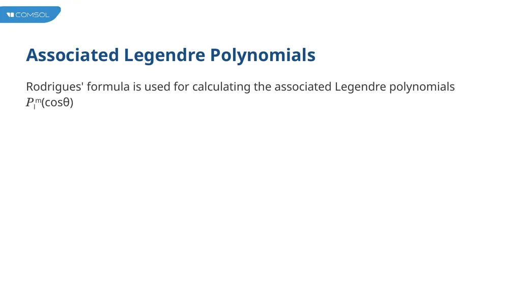
slide8. Associated Legendre Polynomials Rodrigues' formula is used for calculating the associated Legendre polynomials Plm(cosθ)<br>
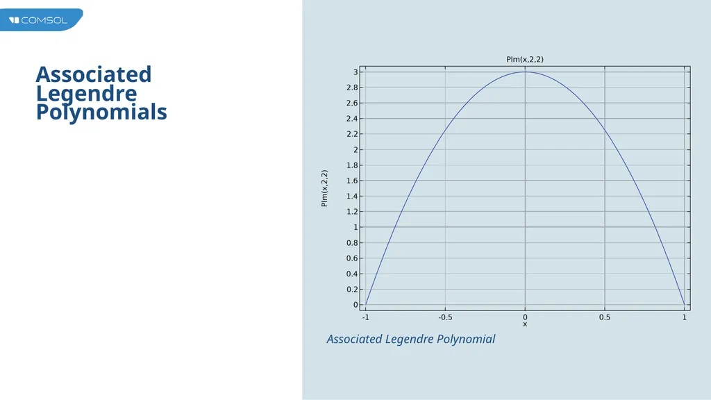
slide9. Associated Legendre Polynomials Associated Legendre Polynomial<br>
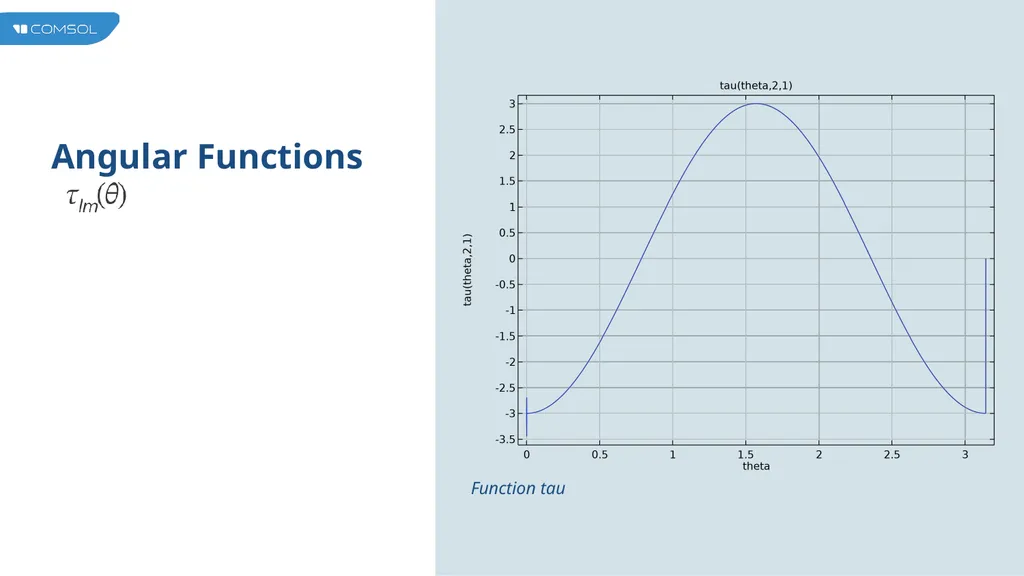
slide10. Angular Functions Function tau<br>
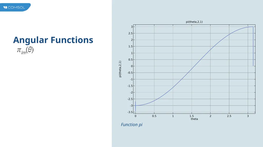
slide11. Angular Functions Function pi<br>
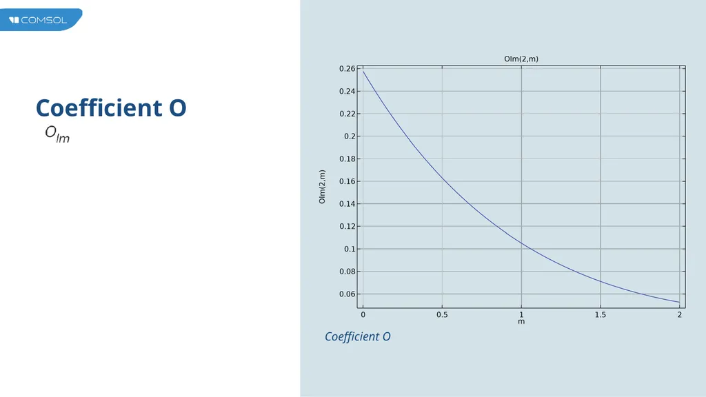
slide12. Coefficient O Coefficient O<br>
slide13. Multipole Variables Calculation of aE(l,1) and aM(l,1)
Defined under Component 1 > Definitions<br>
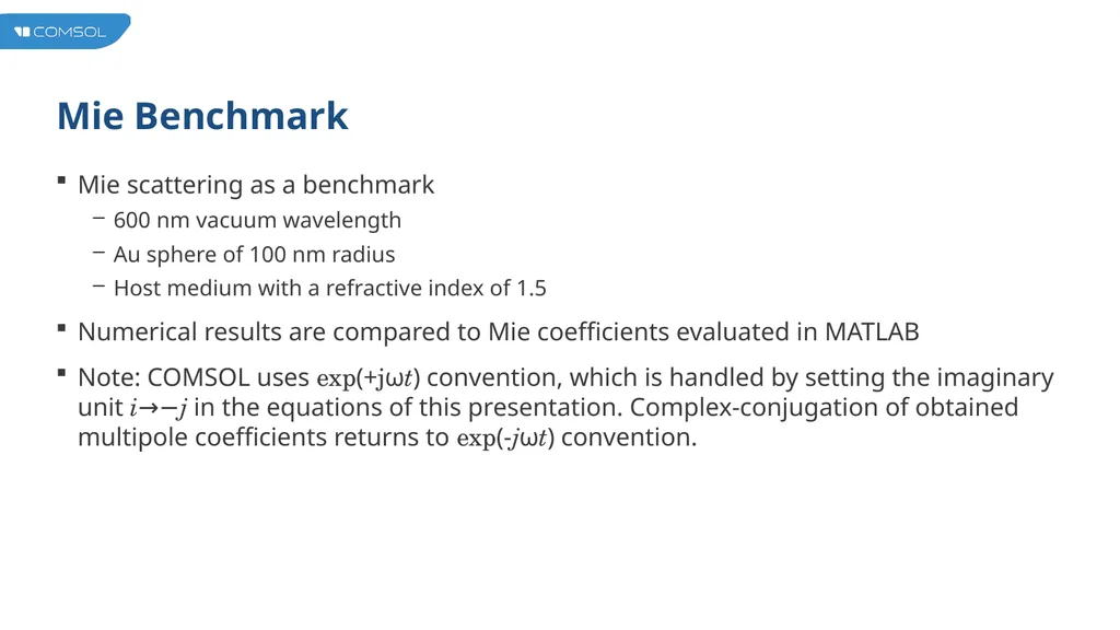
slide14. Mie Benchmark Mie scattering as a benchmark
600 nm vacuum wavelength
Au sphere of 100 nm radius
Host medium with a refractive index of 1.5
Numerical results are compared to Mie coefficients evaluated in MATLAB
Note: COMSOL uses exp(+jωt) convention, which is handled by setting the imaginary unit i→−j in the equations of this presentation. Complex-conjugation of obtained multipole coefficients returns to exp(-jωt) convention.<br>
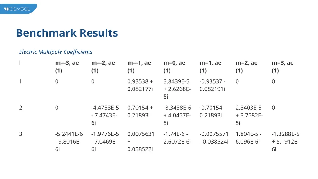
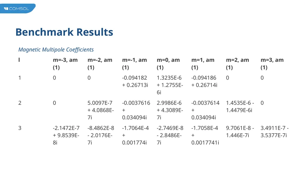
slide15. Benchmark Results<br>
slide16. Benchmark Results<br>
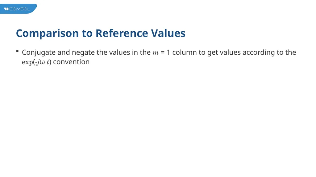
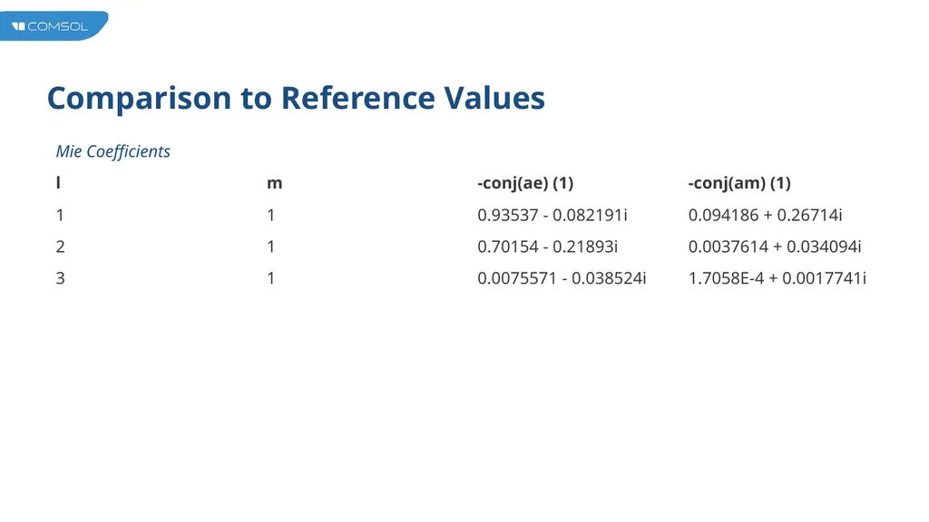
slide17. Comparison to Reference Values Conjugate and negate the values in the m = 1 column to get values according to the exp(-jω t) convention<br>
slide18. Comparison to Reference Values<br>
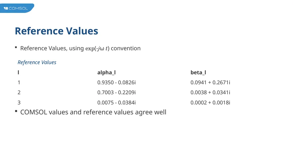
slide19. Reference Values Reference Values, using exp(-jω t) convention COMSOL values and reference values agree well<br>
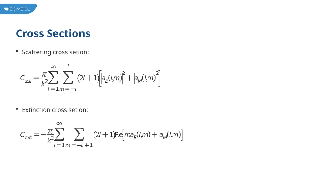
slide20. Cross Sections Scattering cross setion: Extinction cross setion:<br>
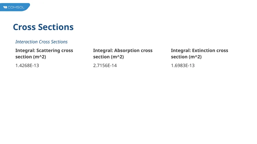
slide21. Cross Sections<br>
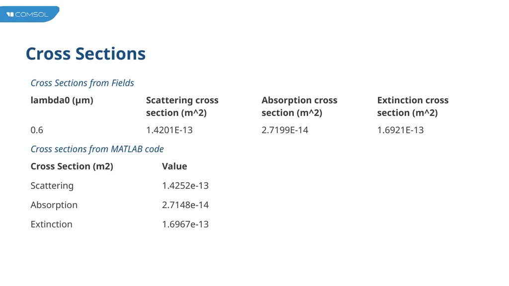
slide22. Cross Sections<br>
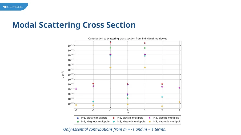
slide23. Modal Scattering Cross Section Only essential contributions from m = -1 and m = 1 terms.<br>
slide24. References J. D. Jackson, Classical Electrodynamics, 3rd Ed., Wiley, 1999.
P. Grahn, A. Shevchenko, and M. Kaivola, "Electromagnetic multipole theory for optical nanomaterials," New Journal of Physics, vol. 14, no. 9, p. 093033, 2012.
C. Mätzler, "MATLAB functions for Mie scattering and absorption, version 2," in IAP Research Report, University of Bern, 2002.<br>

slide2. Multipole Expansion The field scattered by a particle, regardless of the particle’s geometrical shape or composition, can always be expressed through the multipole expansion. The expression for the electric field reads (see Ref. 1): The vector functions<br>
slide3. Multipole Expansion and generate a complete basis, where each function describes the field created by a unique multipole.<br>
slide4. Multipole Coefficients The coefficients aE(l,m) and aM(l,m) characterize the scatterer as they reveal the electric and magnetic excitations in it.
The integer l describes the order of the multipole (dipole, quadrupole, …), whereas the subscripts E and M distinguish between electric and magnetic multipoles. The integer m describes the amount of the z-component of angular momentum that is carried per photon.<br>
slide5. Multipole Coefficients For optical scatterers, the source of the scattered field is the scattering current density where eh is the permittivity of the host medium and E(r) is the total field.
The multipole coefficients can be extracted from the scattering current density, using volume integrals over the whole space (see Ref. 2).<br>
slide6. Mie Scattering Scattering of a plane wave by a spherical particle.
Analytical solution exists as an expansion, in which the coefficients are called Mie coefficients.
MATLAB code (see Ref. 3) exists for computing the Mie coefficients (al and bl).
The Mie expansion is a special case of the Multipole expansion, obtained by setting
all coefficients to zero, if not |m| = 1
aE(l,-1) = -aE(l,1)
aM(l,-1) = aM(l,1)
Connection between the remaining multipole coefficients and the Mie coefficients is
aE(l,1) = -al
aM(l,1) = -bl<br>
slide7. COMSOL Implementation Equations for extracting aE(l,1) and aM(l,1) are implemented in COMSOL using functions and variables
Implementation can be added to any scattering model
Also applicable to periodic systems<br>
slide8. Associated Legendre Polynomials Rodrigues' formula is used for calculating the associated Legendre polynomials Plm(cosθ)<br>
slide9. Associated Legendre Polynomials Associated Legendre Polynomial<br>
slide10. Angular Functions Function tau<br>
slide11. Angular Functions Function pi<br>
slide12. Coefficient O Coefficient O<br>
slide13. Multipole Variables Calculation of aE(l,1) and aM(l,1)
Defined under Component 1 > Definitions<br>
slide14. Mie Benchmark Mie scattering as a benchmark
600 nm vacuum wavelength
Au sphere of 100 nm radius
Host medium with a refractive index of 1.5
Numerical results are compared to Mie coefficients evaluated in MATLAB
Note: COMSOL uses exp(+jωt) convention, which is handled by setting the imaginary unit i→−j in the equations of this presentation. Complex-conjugation of obtained multipole coefficients returns to exp(-jωt) convention.<br>
slide15. Benchmark Results<br>
slide16. Benchmark Results<br>
slide17. Comparison to Reference Values Conjugate and negate the values in the m = 1 column to get values according to the exp(-jω t) convention<br>
slide18. Comparison to Reference Values<br>
slide19. Reference Values Reference Values, using exp(-jω t) convention COMSOL values and reference values agree well<br>
slide20. Cross Sections Scattering cross setion: Extinction cross setion:<br>
slide21. Cross Sections<br>
slide22. Cross Sections<br>
slide23. Modal Scattering Cross Section Only essential contributions from m = -1 and m = 1 terms.<br>
slide24. References J. D. Jackson, Classical Electrodynamics, 3rd Ed., Wiley, 1999.
P. Grahn, A. Shevchenko, and M. Kaivola, "Electromagnetic multipole theory for optical nanomaterials," New Journal of Physics, vol. 14, no. 9, p. 093033, 2012.
C. Mätzler, "MATLAB functions for Mie scattering and absorption, version 2," in IAP Research Report, University of Bern, 2002.<br>