Neural Networks for Machine Learning Lecture 3a
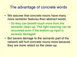
Author : lois-ondreau | Published Date : 2025-05-23
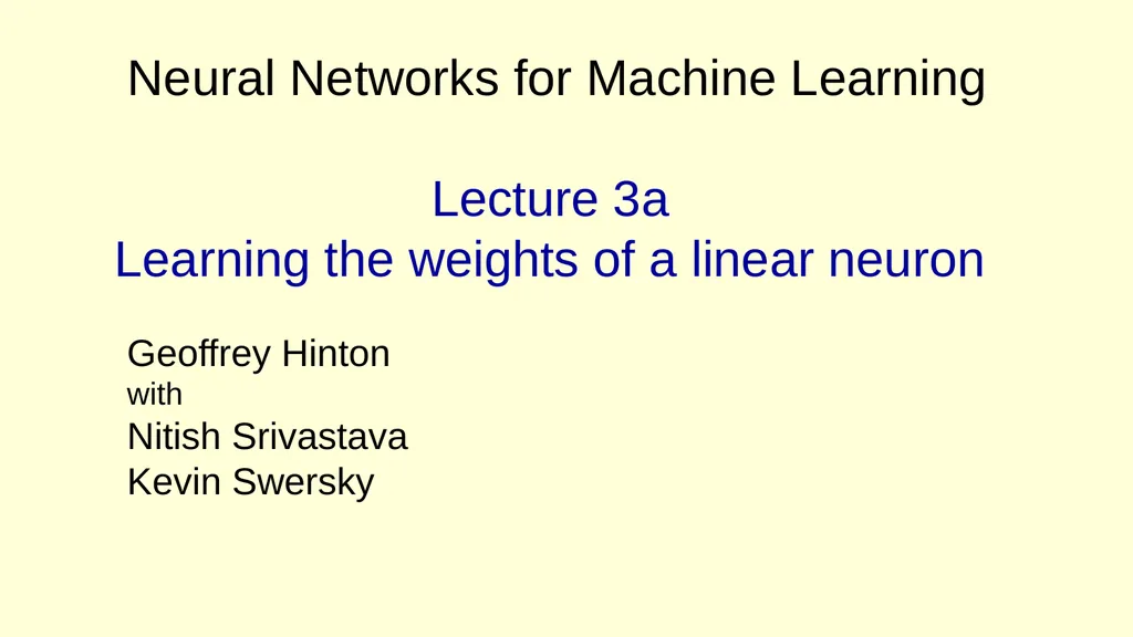
Description: Neural Networks for Machine Learning Lecture 3a Learning the weights of a linear neuron Geoffrey Hinton with Nitish Srivastava Kevin Swersky Why the perceptron learning procedure cannot be generalised to hidden layers The perceptron
Presentation Embed Code
Download Presentation
Download
Presentation The PPT/PDF document
"Neural Networks for Machine Learning Lecture 3a" is the property of its rightful owner.
Permission is granted to download and print the materials on this website for personal, non-commercial use only,
and to display it on your personal computer provided you do not modify the materials and that you retain all
copyright notices contained in the materials. By downloading content from our website, you accept the terms of
this agreement.
Transcript:Neural Networks for Machine Learning Lecture 3a:
Neural Networks for Machine Learning Lecture 3a Learning the weights of a linear neuron Geoffrey Hinton with Nitish Srivastava Kevin Swersky Why the perceptron learning procedure cannot be generalised to hidden layers The perceptron convergence procedure works by ensuring that every time the weights change, they get closer to every “generously feasible” set of weights. This type of guarantee cannot be extended to more complex networks in which the average of two good solutions may be a bad solution. So “multi-layer” neural networks do not use the perceptron learning procedure. They should never have been called multi-layer perceptrons. A different way to show that a learning procedure makes progress Instead of showing the weights get closer to a good set of weights, show that the actual output values get closer the target values. This can be true even for non-convex problems in which there are many quite different sets of weights that work well and averaging two good sets of weights may give a bad set of weights. It is not true for perceptron learning. The simplest example is a linear neuron with a squared error measure. Linear neurons (also called linear filters) The neuron has a real-valued output which is a weighted sum of its inputs The aim of learning is to minimize the error summed over all training cases. The error is the squared difference between the desired output and the actual output. neuron’s estimate of the desired output input vector weight vector Why don’t we solve it analytically? It is straight-forward to write down a set of equations, one per training case, and to solve for the best set of weights. This is the standard engineering approach so why don’t we use it? Scientific answer: We want a method that real neurons could use. Engineering answer: We want a method that can be generalized to multi-layer, non-linear neural networks. The analytic solution relies on it being linear and having a squared error measure. Iterative methods are usually less efficient but they are much easier to generalize. A toy example to illustrate the iterative method Each day you get lunch at the cafeteria. Your diet consists of fish, chips, and ketchup. You get several portions of each. The cashier only tells you the total price of the meal After several days, you should be able to figure out the price of each portion. The iterative approach: Start with