Neural Networks NNs are a study of parallel and

Transcript:Neural Networks NNs are a study of parallel and:
Neural Networks NNs are a study of parallel and distributed processing systems (PDPs) the idea is that the representation is distributed across a network structure an individual node itself does not have meaning, or does not represent a concept, unlike a semantic network NN terminology is similar to that of neurology, but don’t confuse a NN and the brain, there are far more differences than similarities 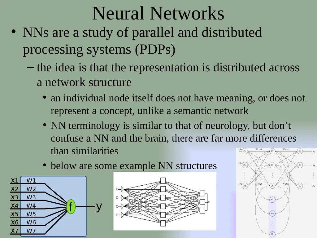below are some example NN structures NN Appeal They are trained rather than programmed so development does not entail the cost of an expert system They provide a form of graceful degradation if part of the representation is damaged (destroyed, removed), the performance degrades “gracefully” rather than completely as with a brittle expert system which might lack the proper knowledge They are particularly useful at solving certain classes of problems low-level classification/recognition optimization content addressable memory Most of these problems are very difficult to solve by expert system Inspiration from the Brain NNs are inspired by the structure of neurons in the brain neurons connect to other neurons by synapses neurons will “fire” which sends electrochemical activity to neighboring neurons across synapses if the neuron excites another neuron, then the excited neuron has a greater chance to fire – such a connection (or link) is known as an excitation link if the neuron inhibits another neuron, then the inhibited neuron has less of a chance to fire – this is an inhibition link NNs Are Not Brains The NN uses the idea of “spreading activation” to determine which nodes fire and which nodes do not The NN learns whether a node should excite or inhibit another node by adjusting the edge weights on the link between them but this analogy should not be taken too far! NNs differ greatly in structure and learning algorithms, we will explore the earliest form for an introduction before looking at several newer and more useful forms the interesting aspects, as noted, are that NNs are trained rather than programmed that they are superior at solving certain low-level tasks than symbolic systems that they can achieve graceful degradation An Artificial Neuron A neural network is a collection of artificial neurons the neuron responds to input, in this case coming from x1, x2, …, xn the neuron computes its output value, denoted here as f(net) the computation for f(net) takes the values of the inputs and multiplies each input by