
Non-experimental methods for transport impact

Description: Non-experimental methods for transport impact evaluation overview In this sessions, we will discuss: the logic of impact evaluation The various methods of non-experimental impact evaluation A case study, to which all major non-experimental
Related Topics
Download Presentation
"Non-experimental methods for transport impact" is the property of its rightful owner. Permission is granted to download and print the materials on this website for personal, non-commercial use only, and to display it on your personal computer provided you do not modify the materials and that you retain all copyright notices contained in the materials. By downloading content from our website, you accept the terms of this agreement.
Presentation Transcript
slide1. Non-experimental methods for transport impact evaluation<br>
slide2. overview In this sessions, we will discuss:
the logic of impact evaluation
The various methods of non-experimental impact evaluation
A case study, to which all major non-experimental methods will be applied<br>
slide3. overview Today: non-experimental methods for impact evaluation
Tomorrow: randomized controlled trials (RCTs)
Wednesday: sampling and power calculations for impact evaluation<br>
slide4. Why impact evaluation? We want to implement the most effective policies and programs
So we need a method that enables us to understand what works and what does not work
The means we need to understand cause and effect
We must measure what happened
We must also find a way to measure the counterfactual (what would have happened if we had not implemented the program)<br>
slide5. M&E versus impact evaluation Monitoring and evaluation
Tracks whether project activities were conducted (inputs)
Counts the project outputs that were delivered/constructed
Was the road built? Was it on time, and did it meet technical standards?
Are people/vehicles using the road?<br>
slide6. M&E versus impact evaluation This standard M&E approach remains very important
But it does not tell us:
Did the road lead to increased economic growth/reduced poverty?
What is the most precise estimate of this economic growth? How does it compare to alternate uses of scarce resources?
Did all groups benefit? Were their winners and losers? To what extent?<br>
slide7. Causal inference and counterfactuals Fundamentally, to know the effect of our project, we want to observe something that is fundamentally unobservable: the counterfactual
What happened to the village where we built a road, compared to what would have happened to the same village if we did not build the road<br>
slide8. Causal inference and counterfactuals Since we can never observe the same village at the same time both with and without the road, we must use other methods to develop a valid comparison group<br>
slide9. impact evaluation A historical example:
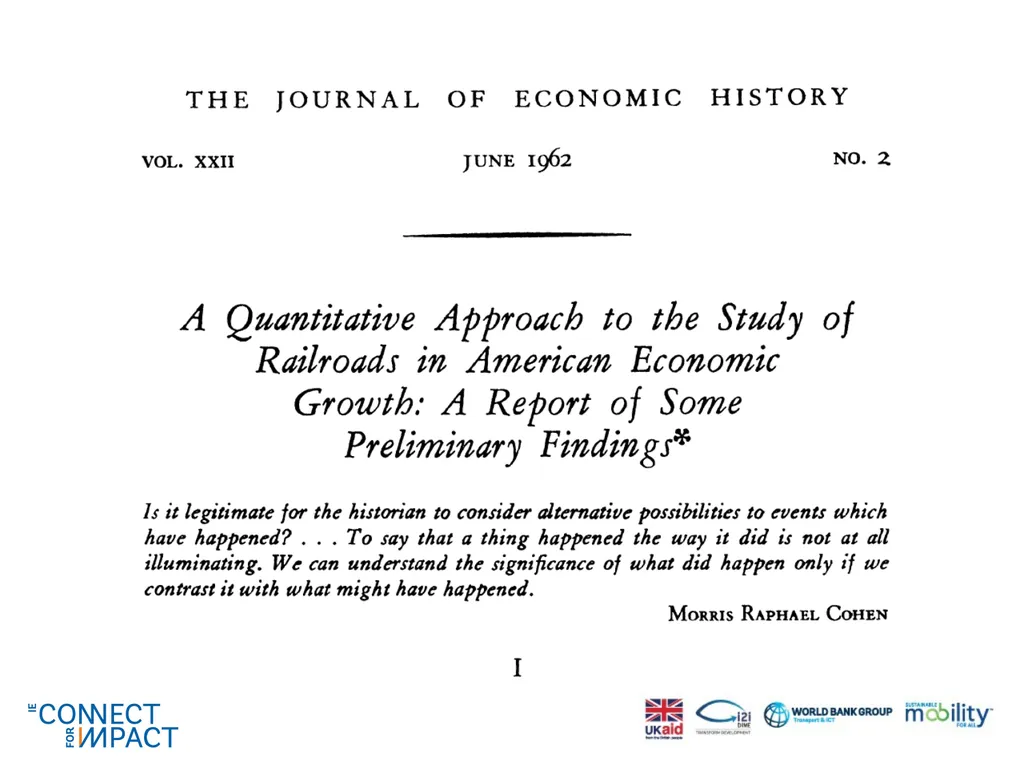
Did the expansion of railways in the late 19th century US contribute to economic growth?
The Fogel hypothesis:<br>
slide11. Building a road (or a railroad) is probably a good thing. But how good, relative to other investments?
“the level of per capita income achieved by January 1, 1890 would have been reached by March 31, 1890, if railroads had never been invented.” Source: Lance Davis, https://eh.net/book_reviews/railroads-and-american-economic-growth-essays-in-econometric-history<br>
slide12. By contrast, new data sources and methods give a very different answer. (Donaldson and Hornbeck 2016)<br>
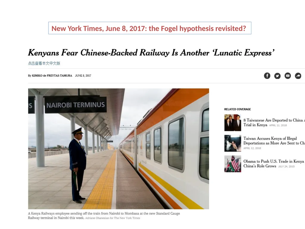
slide13. New York Times, June 8, 2017: the Fogel hypothesis revisited?<br>
slide14. Case study The Republic of Atlantis is planning a rural road rehabilitation program
Agricultural households cannot sell goods at market because poor roads, high transport costs no profit for cash crop production
If you fix the roads, they can produce and sell crops at market -- > higher household incomes and consumption, less poverty<br>
slide15. Case study: the program First they class all villages into groups:
9,000 villages in the country qualify as high priority for road rehabilitation
Given budget limits, the Dept of Transportation opens up the program to 2,000 villages and invites them to apply.
Eligible villages must apply by a certain date, otherwise cannot receive program
By program deadline, 1,021 villages have applied out of 2,000 these villages receive the program<br>
slide16. Case study: the evaluation Minister of Finance:
Roads are expensive – if they want this program to be scaled up, he wants evidence on the economic return
So the team consults with researchers at Atlantis National University on how to design an evaluation that can inform this decision
What is the main question that they must answer with this evaluation?<br>
slide17. Case study: the evaluation Project team has done detailed M&E on previous projects
Tracked that roads were actually built up to standard in project villages
Also measured that, in project villages:
travel time to market centers decreased
Vehicle operating costs for car owners decreased
Did it have any effect incomes or poverty?<br>
slide18. Case study: the evaluation Based on conversation with evaluation team, they improve methods:
Collect information not just about travel times, but collect detailed household consumption data from households
They collect this data in both the program villages (“treatment”) and the comparison villages<br>
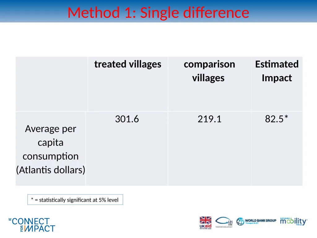
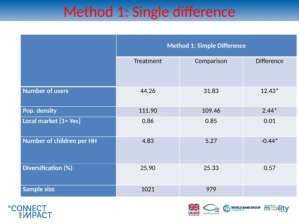
slide19. Method 1: Single difference * = statistically significant at 5% level<br>
slide20. Method 1: Single difference What does this method tell us about the impact of road upgrading on households’ welfare?<br>
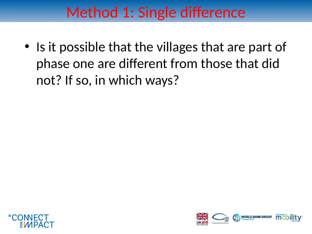
slide21. Method 1: Single difference Is it possible that the villages that are part of phase one are different from those that did not? If so, in which ways?<br>
slide22. Method 1: Single difference<br>
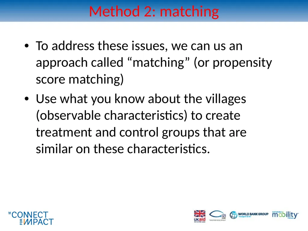
slide23. Method 2: matching To address these issues, we can us an approach called “matching” (or propensity score matching)
Use what you know about the villages (observable characteristics) to create treatment and control groups that are similar on these characteristics.<br>
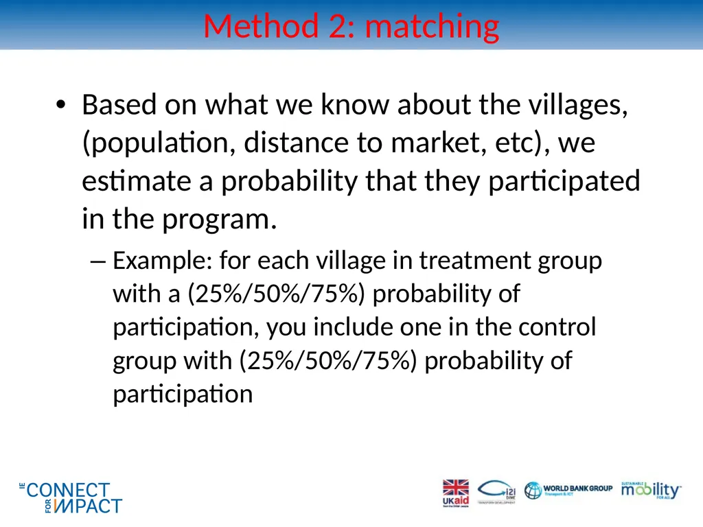
slide24. Method 2: matching Based on what we know about the villages, (population, distance to market, etc), we estimate a probability that they participated in the program.
Example: for each village in treatment group with a (25%/50%/75%) probability of participation, you include one in the control group with (25%/50%/75%) probability of participation<br>
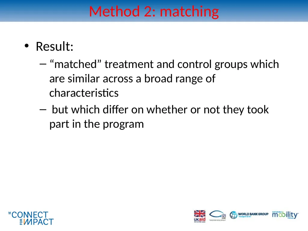
slide25. Method 2: matching Result:
“matched” treatment and control groups which are similar across a broad range of characteristics
but which differ on whether or not they took part in the program<br>
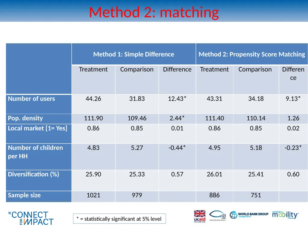
slide26. Method 2: matching * = statistically significant at 5% level<br>
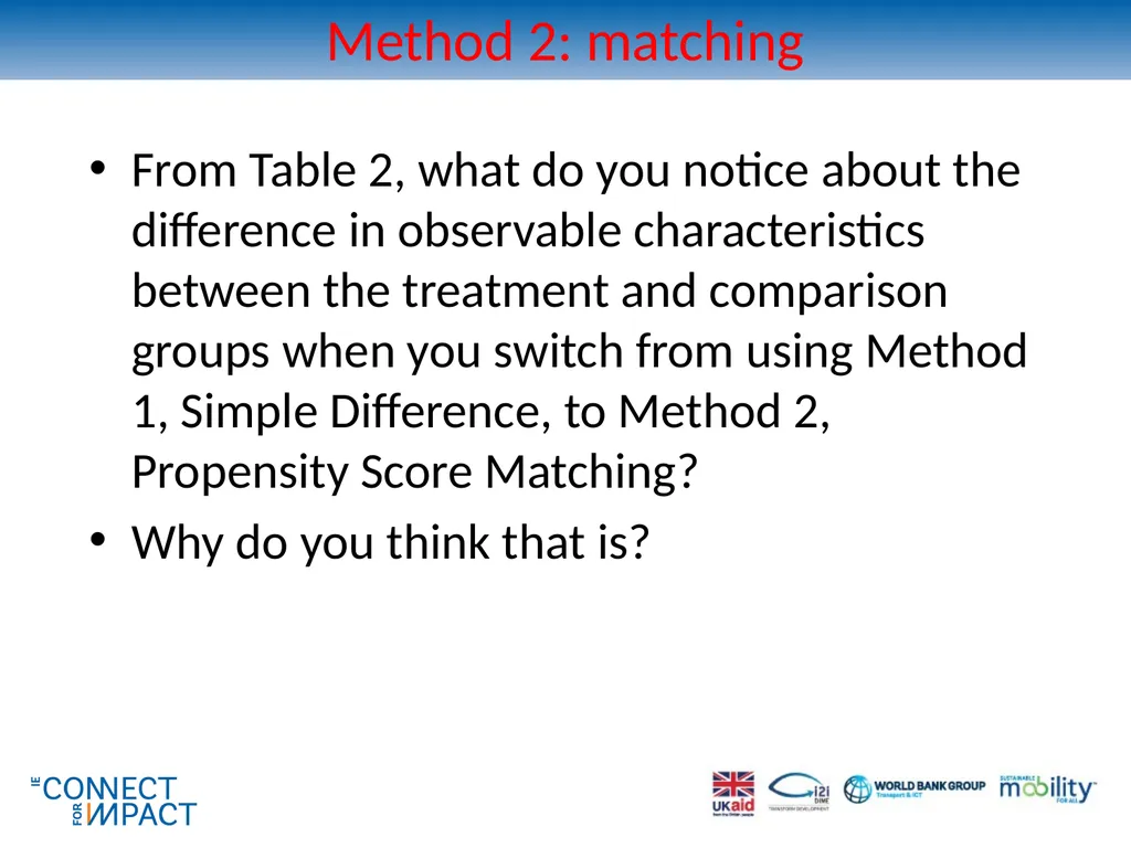
slide27. Method 2: matching From Table 2, what do you notice about the difference in observable characteristics between the treatment and comparison groups when you switch from using Method 1, Simple Difference, to Method 2, Propensity Score Matching?
Why do you think that is?<br>
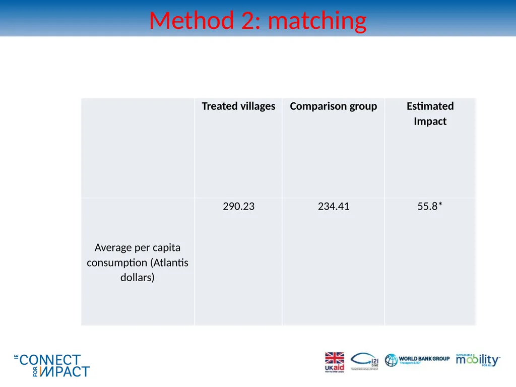
slide28. Method 2: matching<br>
slide29. Method 2: matching Why do you think that the estimated impact of the upgrading using Method 2 is smaller than the impact estimated using Method 1?<br>
slide30. Method 2: matching Notes:
This only accounts for observable traits
May lose sample size
(e.g if you have villages with 99% probability in treatment group but none in control, these will be dropped, and vice versa)<br>
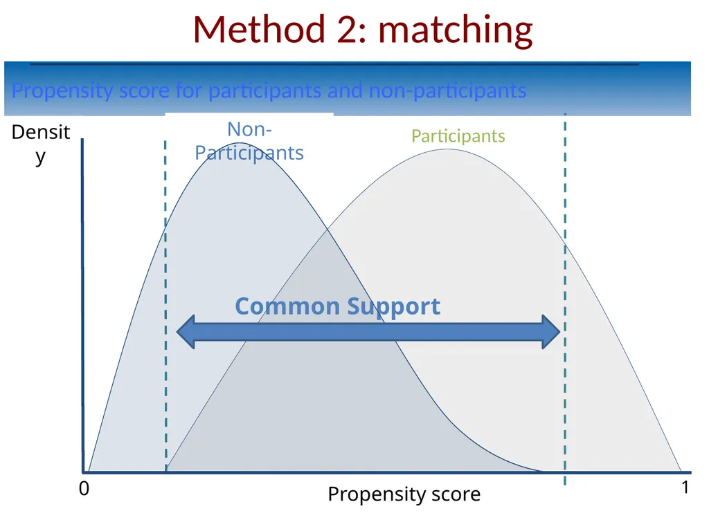
slide31. Propensity score for participants and non-participants Density Propensity score 0 1 Participants Non-Participants Common Support Method 2: matching<br>
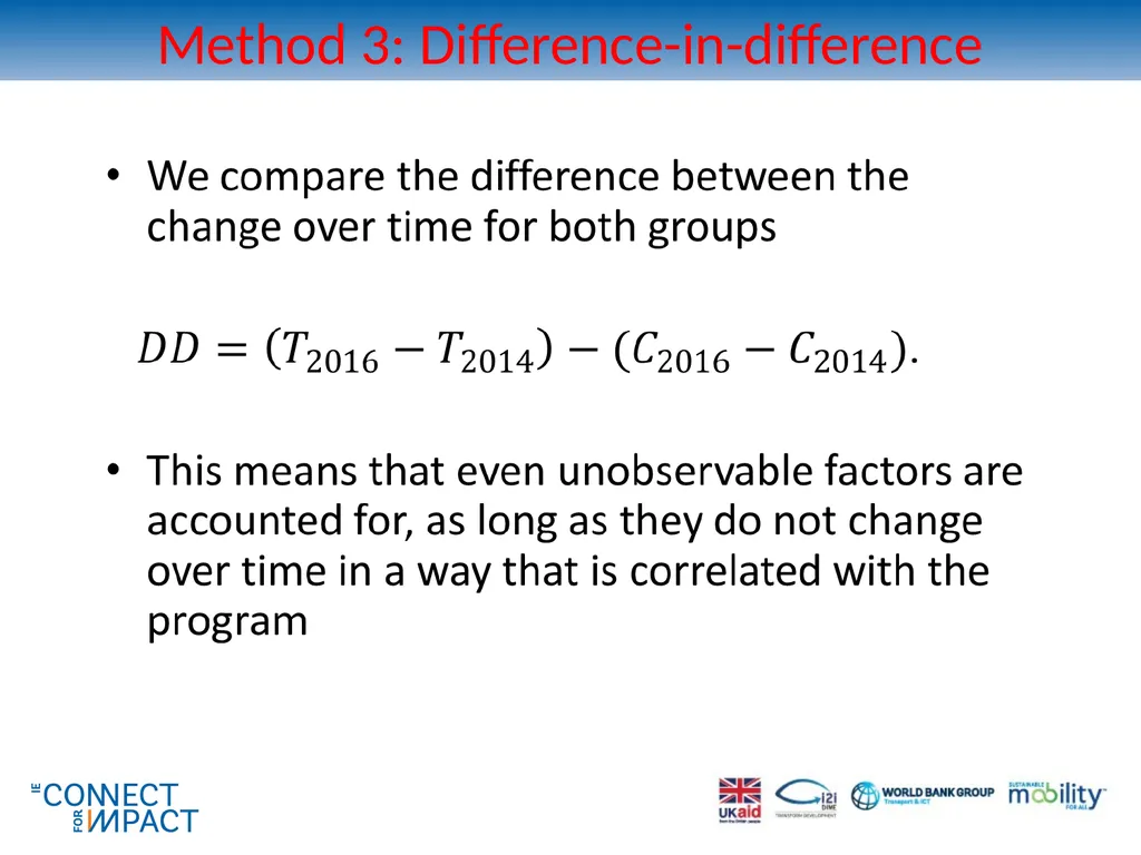
slide32. Method 3: Difference-in-difference There is still the possibility that the two groups are fundamentally different
The difference-in-difference method can help when this is the case.
We measure household consumption before and after the program, and focus on the change over time, rather than the absolute difference<br>
slide33. Method 3: Difference-in-difference<br>
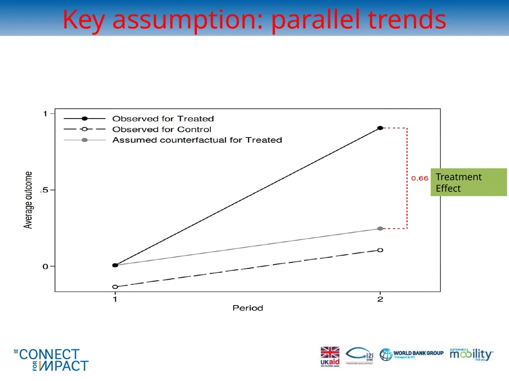
slide34. Key assumption: parallel trends Treatment Effect<br>
slide35. Method 3: Difference-in-difference<br>
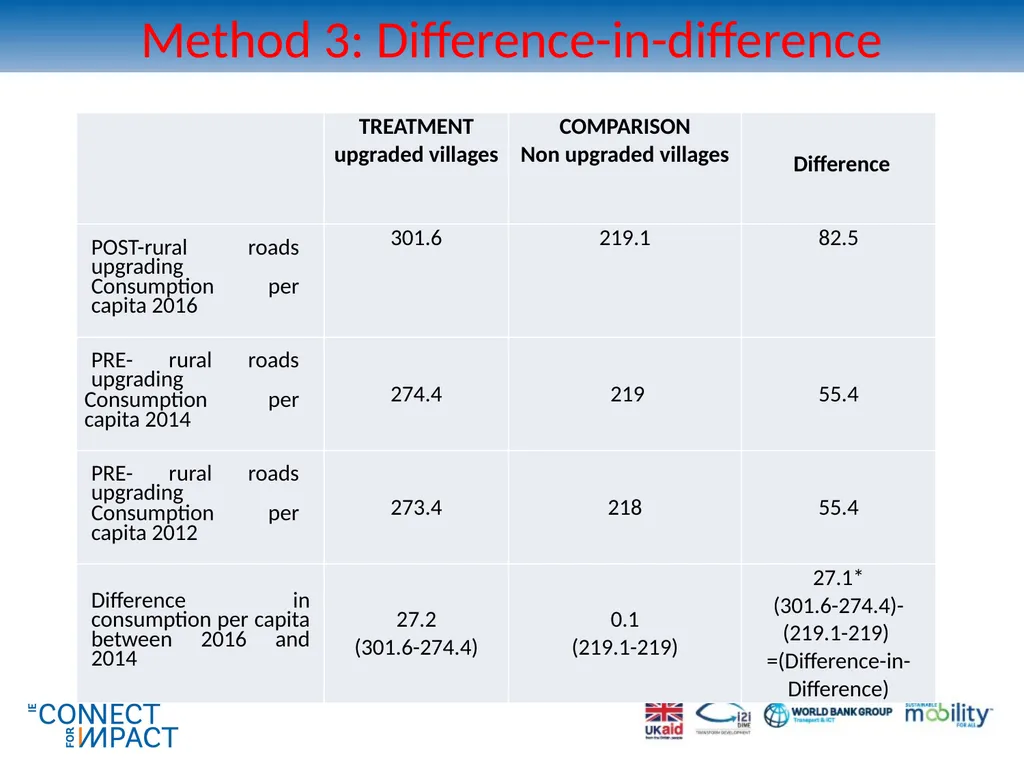
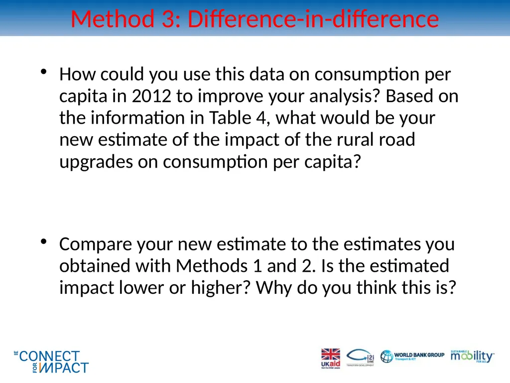
slide36. Method 3: Difference-in-difference How could you use this data on consumption per capita in 2012 to improve your analysis? Based on the information in Table 4, what would be your new estimate of the impact of the rural road upgrades on consumption per capita?
Compare your new estimate to the estimates you obtained with Methods 1 and 2. Is the estimated impact lower or higher? Why do you think this is?<br>
slide37. Method 3: Difference-in-difference Extra notes
Can also use triple difference
matching + DD is a common method
More powerful when there is significant data before treatment so trends can be examined (and controlled for).
important weakness:
Projects often deliberately targeted based on expectations of differential rates of change
“we targeted roads at villages with especially high potential for agricultural growth.”<br>
slide38. Method 4: Regression discontinuity (RD) Now imagine that instead of allocating the road project to villages that applied on time, the team instead ranked eligible villages
based on relevant criteria such as poverty, distance to markets, condition of existing roads
All 2,000 villages are ranked, and all villages with scores above some threshold receive the program, and those below it do not.<br>
slide39. Method 4: Regression discontinuity (RD) Treatment and control will be very different in general, except immediately above and below the threshold
Imagine that the cutoff is 500
Wealthy village near the capital = ranked 995
Poor remote village 1,000 km from capital = ranked 15
These cannot be meaningfully compared<br>
slide40. Method 4: Regression discontinuity (RD) But what about villages 498, 499, 500, 501, 502?
Presence above or below treatment threshold is essentially arbitrary, (close to) random.
Villages 499 and 501 are likely very good comparators for each other<br>
slide41. Method 4: Regression discontinuity (RD) Assignment to the treatment depends on continuous “score” or ranking
observations ordered by looking at the score
there is a cut-off point for “eligibility” – clearly defined criterion determined ex ante
cut-off determines the assignment to treatment<br>
slide42. conclusions High quality non-experimental IE is data-intensive
Advances in big data (remote sensing, high frequency/high resolution administrative data, new survey methods) are making this more feasible
Many examples in forthcoming presentations<br>
slide43. conclusions To design conduct high quality impact evaluations of major transport infrastructure projects, we may need the full toolkit of IE methods<br>
slide44. conclusions In Phase 1 of ieConnect, we have IEs which have:
A non-experimental component which estimates the impact of transport infrastructure (a road, a corridor, a BRT system)
Complementary experimental interventions which test key components of program logic<br>
slide2. overview In this sessions, we will discuss:
the logic of impact evaluation
The various methods of non-experimental impact evaluation
A case study, to which all major non-experimental methods will be applied<br>
slide3. overview Today: non-experimental methods for impact evaluation
Tomorrow: randomized controlled trials (RCTs)
Wednesday: sampling and power calculations for impact evaluation<br>
slide4. Why impact evaluation? We want to implement the most effective policies and programs
So we need a method that enables us to understand what works and what does not work
The means we need to understand cause and effect
We must measure what happened
We must also find a way to measure the counterfactual (what would have happened if we had not implemented the program)<br>
slide5. M&E versus impact evaluation Monitoring and evaluation
Tracks whether project activities were conducted (inputs)
Counts the project outputs that were delivered/constructed
Was the road built? Was it on time, and did it meet technical standards?
Are people/vehicles using the road?<br>
slide6. M&E versus impact evaluation This standard M&E approach remains very important
But it does not tell us:
Did the road lead to increased economic growth/reduced poverty?
What is the most precise estimate of this economic growth? How does it compare to alternate uses of scarce resources?
Did all groups benefit? Were their winners and losers? To what extent?<br>
slide7. Causal inference and counterfactuals Fundamentally, to know the effect of our project, we want to observe something that is fundamentally unobservable: the counterfactual
What happened to the village where we built a road, compared to what would have happened to the same village if we did not build the road<br>
slide8. Causal inference and counterfactuals Since we can never observe the same village at the same time both with and without the road, we must use other methods to develop a valid comparison group<br>
slide9. impact evaluation A historical example:
Did the expansion of railways in the late 19th century US contribute to economic growth?
The Fogel hypothesis:<br>
slide11. Building a road (or a railroad) is probably a good thing. But how good, relative to other investments?
“the level of per capita income achieved by January 1, 1890 would have been reached by March 31, 1890, if railroads had never been invented.” Source: Lance Davis, https://eh.net/book_reviews/railroads-and-american-economic-growth-essays-in-econometric-history<br>
slide12. By contrast, new data sources and methods give a very different answer. (Donaldson and Hornbeck 2016)<br>
slide13. New York Times, June 8, 2017: the Fogel hypothesis revisited?<br>
slide14. Case study The Republic of Atlantis is planning a rural road rehabilitation program
Agricultural households cannot sell goods at market because poor roads, high transport costs no profit for cash crop production
If you fix the roads, they can produce and sell crops at market -- > higher household incomes and consumption, less poverty<br>
slide15. Case study: the program First they class all villages into groups:
9,000 villages in the country qualify as high priority for road rehabilitation
Given budget limits, the Dept of Transportation opens up the program to 2,000 villages and invites them to apply.
Eligible villages must apply by a certain date, otherwise cannot receive program
By program deadline, 1,021 villages have applied out of 2,000 these villages receive the program<br>
slide16. Case study: the evaluation Minister of Finance:
Roads are expensive – if they want this program to be scaled up, he wants evidence on the economic return
So the team consults with researchers at Atlantis National University on how to design an evaluation that can inform this decision
What is the main question that they must answer with this evaluation?<br>
slide17. Case study: the evaluation Project team has done detailed M&E on previous projects
Tracked that roads were actually built up to standard in project villages
Also measured that, in project villages:
travel time to market centers decreased
Vehicle operating costs for car owners decreased
Did it have any effect incomes or poverty?<br>
slide18. Case study: the evaluation Based on conversation with evaluation team, they improve methods:
Collect information not just about travel times, but collect detailed household consumption data from households
They collect this data in both the program villages (“treatment”) and the comparison villages<br>
slide19. Method 1: Single difference * = statistically significant at 5% level<br>
slide20. Method 1: Single difference What does this method tell us about the impact of road upgrading on households’ welfare?<br>
slide21. Method 1: Single difference Is it possible that the villages that are part of phase one are different from those that did not? If so, in which ways?<br>
slide22. Method 1: Single difference<br>
slide23. Method 2: matching To address these issues, we can us an approach called “matching” (or propensity score matching)
Use what you know about the villages (observable characteristics) to create treatment and control groups that are similar on these characteristics.<br>
slide24. Method 2: matching Based on what we know about the villages, (population, distance to market, etc), we estimate a probability that they participated in the program.
Example: for each village in treatment group with a (25%/50%/75%) probability of participation, you include one in the control group with (25%/50%/75%) probability of participation<br>
slide25. Method 2: matching Result:
“matched” treatment and control groups which are similar across a broad range of characteristics
but which differ on whether or not they took part in the program<br>
slide26. Method 2: matching * = statistically significant at 5% level<br>
slide27. Method 2: matching From Table 2, what do you notice about the difference in observable characteristics between the treatment and comparison groups when you switch from using Method 1, Simple Difference, to Method 2, Propensity Score Matching?
Why do you think that is?<br>
slide28. Method 2: matching<br>
slide29. Method 2: matching Why do you think that the estimated impact of the upgrading using Method 2 is smaller than the impact estimated using Method 1?<br>
slide30. Method 2: matching Notes:
This only accounts for observable traits
May lose sample size
(e.g if you have villages with 99% probability in treatment group but none in control, these will be dropped, and vice versa)<br>
slide31. Propensity score for participants and non-participants Density Propensity score 0 1 Participants Non-Participants Common Support Method 2: matching<br>
slide32. Method 3: Difference-in-difference There is still the possibility that the two groups are fundamentally different
The difference-in-difference method can help when this is the case.
We measure household consumption before and after the program, and focus on the change over time, rather than the absolute difference<br>
slide33. Method 3: Difference-in-difference<br>
slide34. Key assumption: parallel trends Treatment Effect<br>
slide35. Method 3: Difference-in-difference<br>
slide36. Method 3: Difference-in-difference How could you use this data on consumption per capita in 2012 to improve your analysis? Based on the information in Table 4, what would be your new estimate of the impact of the rural road upgrades on consumption per capita?
Compare your new estimate to the estimates you obtained with Methods 1 and 2. Is the estimated impact lower or higher? Why do you think this is?<br>
slide37. Method 3: Difference-in-difference Extra notes
Can also use triple difference
matching + DD is a common method
More powerful when there is significant data before treatment so trends can be examined (and controlled for).
important weakness:
Projects often deliberately targeted based on expectations of differential rates of change
“we targeted roads at villages with especially high potential for agricultural growth.”<br>
slide38. Method 4: Regression discontinuity (RD) Now imagine that instead of allocating the road project to villages that applied on time, the team instead ranked eligible villages
based on relevant criteria such as poverty, distance to markets, condition of existing roads
All 2,000 villages are ranked, and all villages with scores above some threshold receive the program, and those below it do not.<br>
slide39. Method 4: Regression discontinuity (RD) Treatment and control will be very different in general, except immediately above and below the threshold
Imagine that the cutoff is 500
Wealthy village near the capital = ranked 995
Poor remote village 1,000 km from capital = ranked 15
These cannot be meaningfully compared<br>
slide40. Method 4: Regression discontinuity (RD) But what about villages 498, 499, 500, 501, 502?
Presence above or below treatment threshold is essentially arbitrary, (close to) random.
Villages 499 and 501 are likely very good comparators for each other<br>
slide41. Method 4: Regression discontinuity (RD) Assignment to the treatment depends on continuous “score” or ranking
observations ordered by looking at the score
there is a cut-off point for “eligibility” – clearly defined criterion determined ex ante
cut-off determines the assignment to treatment<br>
slide42. conclusions High quality non-experimental IE is data-intensive
Advances in big data (remote sensing, high frequency/high resolution administrative data, new survey methods) are making this more feasible
Many examples in forthcoming presentations<br>
slide43. conclusions To design conduct high quality impact evaluations of major transport infrastructure projects, we may need the full toolkit of IE methods<br>
slide44. conclusions In Phase 1 of ieConnect, we have IEs which have:
A non-experimental component which estimates the impact of transport infrastructure (a road, a corridor, a BRT system)
Complementary experimental interventions which test key components of program logic<br>