
Non-Parametric Normalizing Flow Modeling of Binary

Description: Non-Parametric Normalizing Flow Modeling of Binary Black Hole Populations for Unbiased Dark Siren Cosmology Leonardo Iampieri, Simone Mastrogiovanni Paris Workshop - 21052025 Discrepancy in the measured values of the Hubble Constant
Related Topics
Download Presentation
"Non-Parametric Normalizing Flow Modeling of Binary" is the property of its rightful owner. Permission is granted to download and print the materials on this website for personal, non-commercial use only, and to display it on your personal computer provided you do not modify the materials and that you retain all copyright notices contained in the materials. By downloading content from our website, you accept the terms of this agreement.
Presentation Transcript
slide1. Non-Parametric Normalizing Flow Modeling of Binary Black Hole Populations for Unbiased Dark Siren Cosmology
Leonardo Iampieri, Simone Mastrogiovanni
Paris Workshop - 21/05/2025 ‹#›<br>
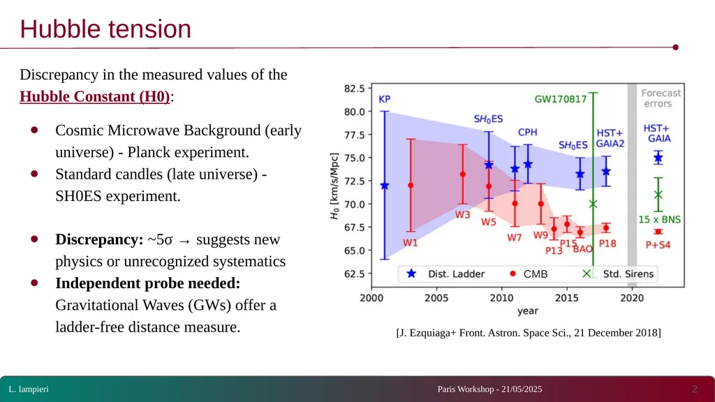
slide2. Discrepancy in the measured values of the Hubble Constant (H0):
Cosmic Microwave Background (early universe) - Planck experiment.
Standard candles (late universe) - SH0ES experiment.
Discrepancy: ~5σ → suggests new physics or unrecognized systematics
Independent probe needed: Gravitational Waves (GWs) offer a ladder-free distance measure. Hubble tension [J. Ezquiaga+ Front. Astron. Space Sci., 21 December 2018] ‹#› L. Iampieri Paris Workshop - 21/05/2025 CMB<br>
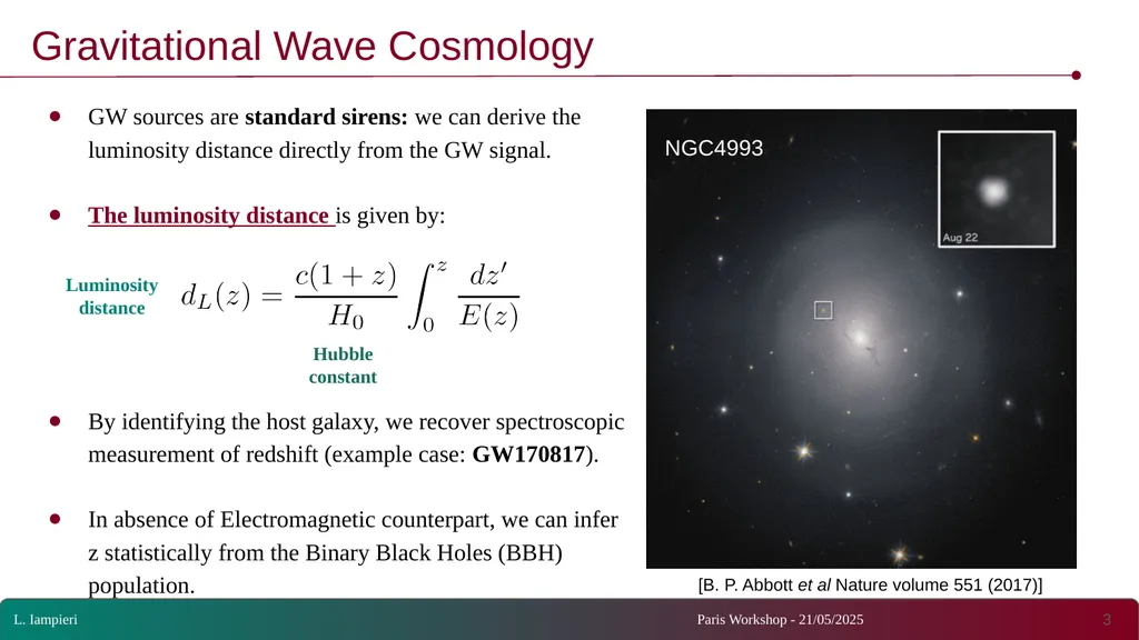
slide3. GW sources are standard sirens: we can derive the luminosity distance directly from the GW signal.
The luminosity distance is given by:
By identifying the host galaxy, we recover spectroscopic measurement of redshift (example case: GW170817).
In absence of Electromagnetic counterpart, we can infer z statistically from the Binary Black Holes (BBH) population. Gravitational Wave Cosmology ‹#› L. Iampieri Paris Workshop - 21/05/2025 Luminosity distance Hubble constant [B. P. Abbott et al Nature volume 551 (2017)] NGC4993<br>
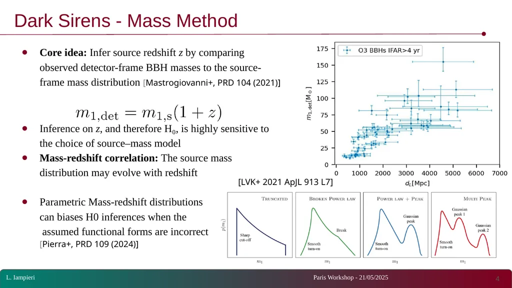
slide4. Core idea: Infer source redshift z by comparing observed detector-frame BBH masses to the source-frame mass distribution [Mastrogiovanni+, PRD 104 (2021)]
Inference on z, and therefore H₀, is highly sensitive to the choice of source–mass model
Mass-redshift correlation: The source mass distribution may evolve with redshift
Parametric Mass-redshift distributions
can biases H0 inferences when the
assumed functional forms are incorrect [Pierra+, PRD 109 (2024)] Dark Sirens - Mass Method ‹#› L. Iampieri Paris Workshop - 21/05/2025 NGC993 [LVK+ 2021 ApJL 913 L7]<br>
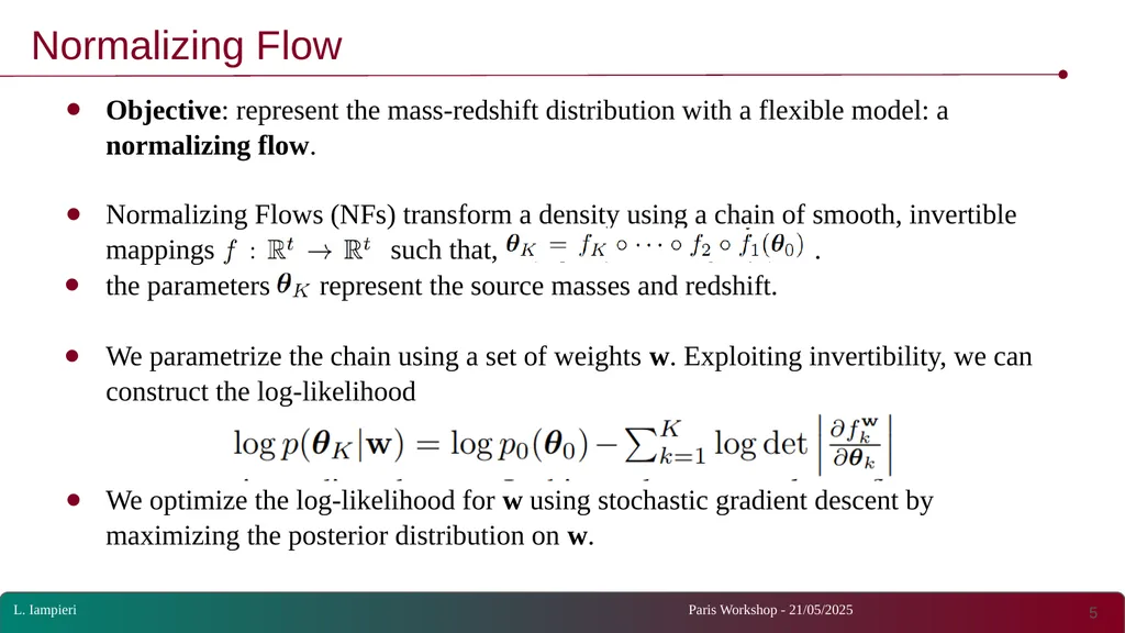
slide5. Objective: represent the mass-redshift distribution with a flexible model: a normalizing flow.
Normalizing Flows (NFs) transform a density using a chain of smooth, invertible mappings such that, .
the parameters represent the source masses and redshift.
We parametrize the chain using a set of weights w. Exploiting invertibility, we can construct the log-likelihood
We optimize the log-likelihood for w using stochastic gradient descent by maximizing the posterior distribution on w. Normalizing Flow ‹#› L. Iampieri Paris Workshop - 21/05/2025<br>
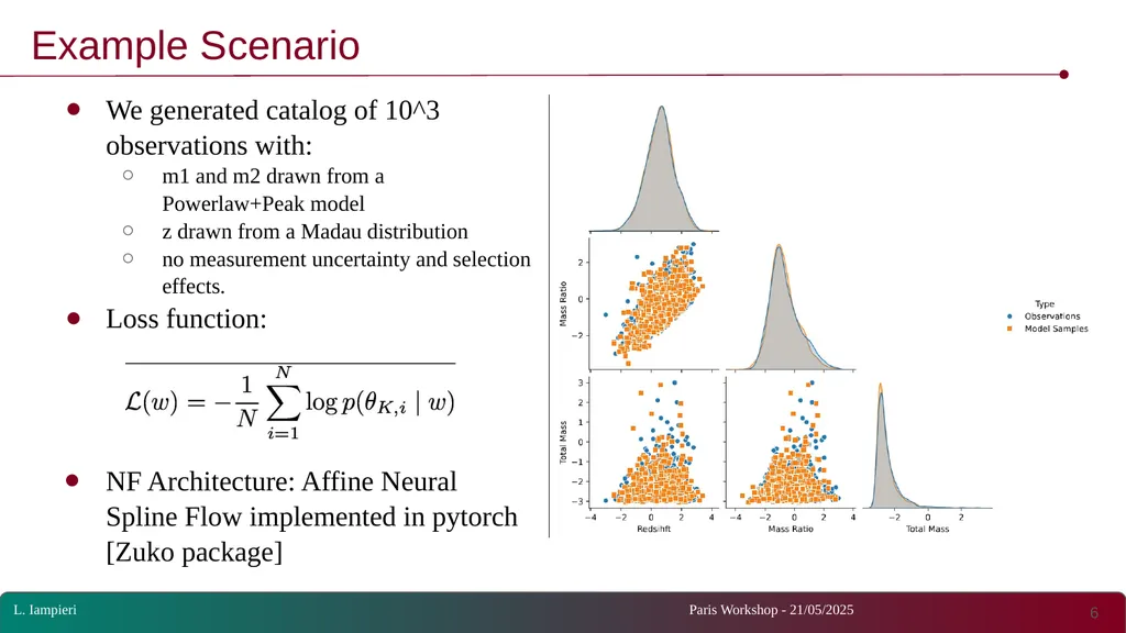
slide6. We generated catalog of 10^3 observations with:
m1 and m2 drawn from a Powerlaw+Peak model
z drawn from a Madau distribution
no measurement uncertainty and selection effects.
Loss function:
NF Architecture: Affine Neural Spline Flow implemented in pytorch [Zuko package] Example Scenario ‹#› L. Iampieri Paris Workshop - 21/05/2025<br>
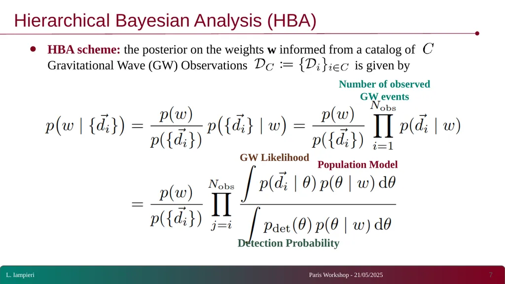
slide7. HBA scheme: the posterior on the weights w informed from a catalog of Gravitational Wave (GW) Observations is given by Hierarchical Bayesian Analysis (HBA) ‹#› L. Iampieri Paris Workshop - 21/05/2025 Detection Probability Population Model GW Likelihood Number of observed GW events<br>
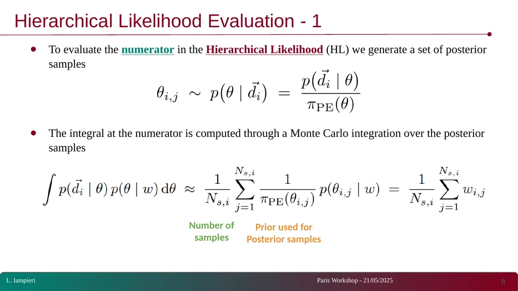
slide8. To evaluate the numerator in the Hierarchical Likelihood (HL) we generate a set of posterior samples
The integral at the numerator is computed through a Monte Carlo integration over the posterior samples Hierarchical Likelihood Evaluation - 1 ‹#› L. Iampieri Paris Workshop - 21/05/2025 Number of samples Prior used for Posterior samples<br>
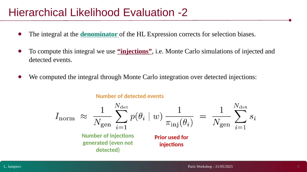
slide9. Hierarchical Likelihood Evaluation -2 ‹#› L. Iampieri Paris Workshop - 21/05/2025 The integral at the denominator of the HL Expression corrects for selection biases.
To compute this integral we use “injections”, i.e. Monte Carlo simulations of injected and detected events.
We computed the integral through Monte Carlo integration over detected injections: Number of detected events Number of injections generated (even not detected) Prior used for injections<br>
slide10. In the presence of noise uncertainty and selection biases, the loss to minimize becomes Loss Function ‹#› L. Iampieri Paris Workshop - 21/05/2025 Number of PE samples Prior used for Posterior samples Prior used for injections Number of total injections Number of detected injections Number of observations<br>
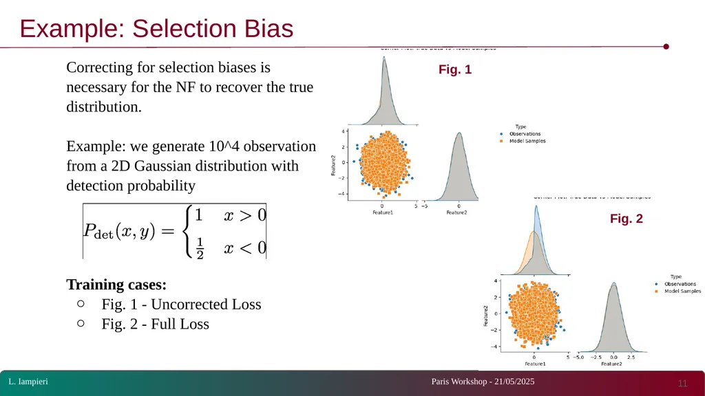
slide11. Correcting for selection biases is necessary for the NF to recover the true distribution.
Example: we generate 10^4 observation from a 2D Gaussian distribution with detection probability
Training cases:
Fig. 1 - Uncorrected Loss
Fig. 2 - Full Loss Example: Selection Bias ‹#› L. Iampieri Paris Workshop - 21/05/2025 Fig. 1 Fig. 2<br>
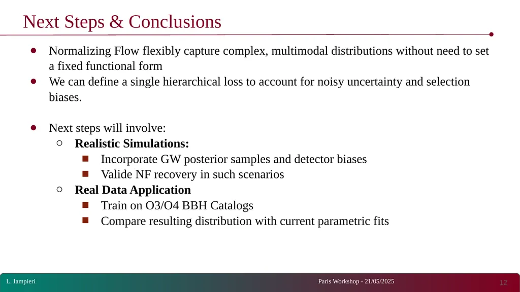
slide12. Next Steps & Conclusions Normalizing Flow flexibly capture complex, multimodal distributions without need to set a fixed functional form
We can define a single hierarchical loss to account for noisy uncertainty and selection biases.
Next steps will involve:
Realistic Simulations:
Incorporate GW posterior samples and detector biases
Valide NF recovery in such scenarios
Real Data Application
Train on O3/O4 BBH Catalogs
Compare resulting distribution with current parametric fits ‹#› L. Iampieri Paris Workshop - 21/05/2025<br>
Leonardo Iampieri, Simone Mastrogiovanni
Paris Workshop - 21/05/2025 ‹#›<br>
slide2. Discrepancy in the measured values of the Hubble Constant (H0):
Cosmic Microwave Background (early universe) - Planck experiment.
Standard candles (late universe) - SH0ES experiment.
Discrepancy: ~5σ → suggests new physics or unrecognized systematics
Independent probe needed: Gravitational Waves (GWs) offer a ladder-free distance measure. Hubble tension [J. Ezquiaga+ Front. Astron. Space Sci., 21 December 2018] ‹#› L. Iampieri Paris Workshop - 21/05/2025 CMB<br>
slide3. GW sources are standard sirens: we can derive the luminosity distance directly from the GW signal.
The luminosity distance is given by:
By identifying the host galaxy, we recover spectroscopic measurement of redshift (example case: GW170817).
In absence of Electromagnetic counterpart, we can infer z statistically from the Binary Black Holes (BBH) population. Gravitational Wave Cosmology ‹#› L. Iampieri Paris Workshop - 21/05/2025 Luminosity distance Hubble constant [B. P. Abbott et al Nature volume 551 (2017)] NGC4993<br>
slide4. Core idea: Infer source redshift z by comparing observed detector-frame BBH masses to the source-frame mass distribution [Mastrogiovanni+, PRD 104 (2021)]
Inference on z, and therefore H₀, is highly sensitive to the choice of source–mass model
Mass-redshift correlation: The source mass distribution may evolve with redshift
Parametric Mass-redshift distributions
can biases H0 inferences when the
assumed functional forms are incorrect [Pierra+, PRD 109 (2024)] Dark Sirens - Mass Method ‹#› L. Iampieri Paris Workshop - 21/05/2025 NGC993 [LVK+ 2021 ApJL 913 L7]<br>
slide5. Objective: represent the mass-redshift distribution with a flexible model: a normalizing flow.
Normalizing Flows (NFs) transform a density using a chain of smooth, invertible mappings such that, .
the parameters represent the source masses and redshift.
We parametrize the chain using a set of weights w. Exploiting invertibility, we can construct the log-likelihood
We optimize the log-likelihood for w using stochastic gradient descent by maximizing the posterior distribution on w. Normalizing Flow ‹#› L. Iampieri Paris Workshop - 21/05/2025<br>
slide6. We generated catalog of 10^3 observations with:
m1 and m2 drawn from a Powerlaw+Peak model
z drawn from a Madau distribution
no measurement uncertainty and selection effects.
Loss function:
NF Architecture: Affine Neural Spline Flow implemented in pytorch [Zuko package] Example Scenario ‹#› L. Iampieri Paris Workshop - 21/05/2025<br>
slide7. HBA scheme: the posterior on the weights w informed from a catalog of Gravitational Wave (GW) Observations is given by Hierarchical Bayesian Analysis (HBA) ‹#› L. Iampieri Paris Workshop - 21/05/2025 Detection Probability Population Model GW Likelihood Number of observed GW events<br>
slide8. To evaluate the numerator in the Hierarchical Likelihood (HL) we generate a set of posterior samples
The integral at the numerator is computed through a Monte Carlo integration over the posterior samples Hierarchical Likelihood Evaluation - 1 ‹#› L. Iampieri Paris Workshop - 21/05/2025 Number of samples Prior used for Posterior samples<br>
slide9. Hierarchical Likelihood Evaluation -2 ‹#› L. Iampieri Paris Workshop - 21/05/2025 The integral at the denominator of the HL Expression corrects for selection biases.
To compute this integral we use “injections”, i.e. Monte Carlo simulations of injected and detected events.
We computed the integral through Monte Carlo integration over detected injections: Number of detected events Number of injections generated (even not detected) Prior used for injections<br>
slide10. In the presence of noise uncertainty and selection biases, the loss to minimize becomes Loss Function ‹#› L. Iampieri Paris Workshop - 21/05/2025 Number of PE samples Prior used for Posterior samples Prior used for injections Number of total injections Number of detected injections Number of observations<br>
slide11. Correcting for selection biases is necessary for the NF to recover the true distribution.
Example: we generate 10^4 observation from a 2D Gaussian distribution with detection probability
Training cases:
Fig. 1 - Uncorrected Loss
Fig. 2 - Full Loss Example: Selection Bias ‹#› L. Iampieri Paris Workshop - 21/05/2025 Fig. 1 Fig. 2<br>
slide12. Next Steps & Conclusions Normalizing Flow flexibly capture complex, multimodal distributions without need to set a fixed functional form
We can define a single hierarchical loss to account for noisy uncertainty and selection biases.
Next steps will involve:
Realistic Simulations:
Incorporate GW posterior samples and detector biases
Valide NF recovery in such scenarios
Real Data Application
Train on O3/O4 BBH Catalogs
Compare resulting distribution with current parametric fits ‹#› L. Iampieri Paris Workshop - 21/05/2025<br>