Open-Channel Flow Contents Free surface flow

slide1. Open-Channel Flow Contents
Free surface flow –basic concepts
Velocity and Pressure Distribution
Energy and Momentum Principles
GRADUALLY VARIED FLOW GVF.
RAPIDLY VARIED FLOW RVF.
UNSTEADY FLOW.
Chapter one Preface
Open channel flow occurs when a liquid flowing due to gravity is only partial enclosed by its solid boundary. The flow in an open channel or in a closed conduit<br>
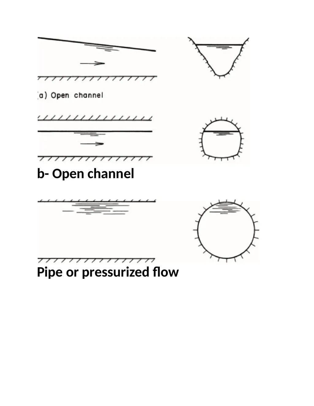
slide2. having a free surface is referred to as free-surface flow or open-channel flow. Here the only force affected is the gravitational force. Some open channel flow occurs naturally as in the case of creeks and rivers, which have generally irregular cross sections A varies with depth. occurs Open channel flow may also in artificial (i.e human construction) channels such as flumes and canals. If there is no free surface and the conduit is flowing full, then the flow is called pipe flow, or pressurized flow.<br>
slide3. b- Open channel Pipe or pressurized flow<br>
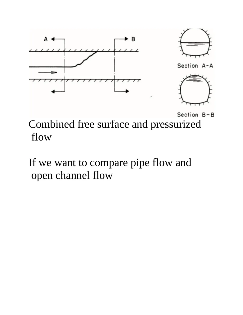
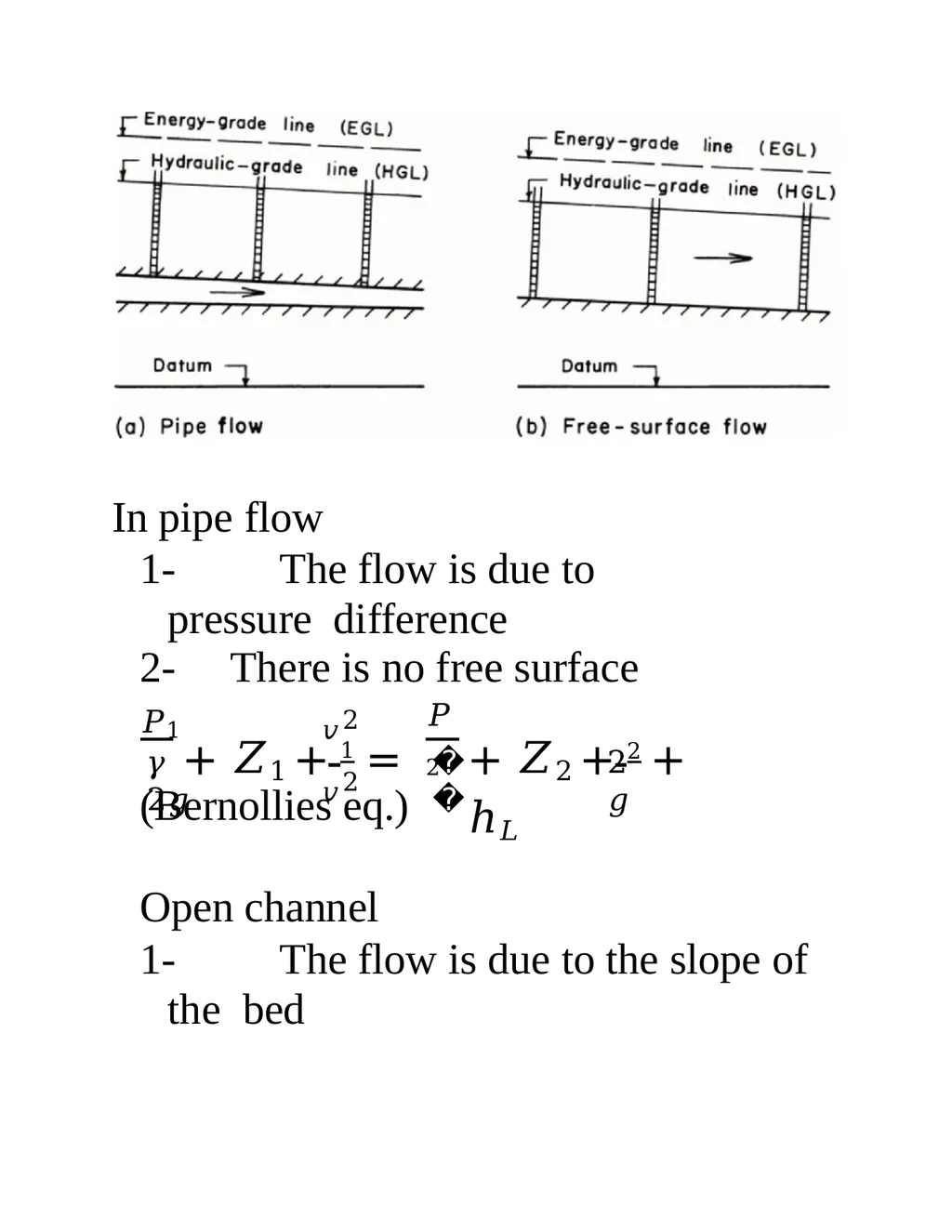
slide4. Combined free surface and pressurized flow If we want to compare pipe flow and open channel flow<br>
slide5. In pipe flow 1- The flow is due to pressure difference 2- There is no free surface
𝑃1 𝛾 2𝑔 + 𝑍1 + 1 = 𝑃2 𝛾 𝑣2 𝑣2 2𝑔 + 𝑍2 + 2 + ℎ𝐿 (Bernollies eq.)

Open channel
1- The flow is due to the slope of the bed<br>
slide6. 2- The hydraulic line is the water 𝟏 𝟏 𝟐𝒈 𝟐 𝟐 surface
3- The pressure is atmospheric
The same eq. applied on open channel
𝒗𝟐 𝒗𝟐 𝟐𝒈 𝒚 + 𝒁 + 𝟏 = 𝒚 + 𝒁 + 𝟐 + 𝒉 𝑳 𝒑
𝜸 = 𝒑𝒓𝒆𝒔𝒔𝒖𝒓𝒆 𝒇𝒐𝒓𝒄𝒆 (𝒎) Z= gravity force , V2/2g= inertia force (velocity head), hL= losses or viscous force

Classification of flow in open channels Based on different criteria, free-surface flows may be classified into various types
1- Steady and Unsteady Flows<br>
slide7. If the flow velocity at a given point does not change with respect to time, then the flow is called steady flow. However, if the velocity at a given location changes with respect to time, then the flow is called unsteady flow.
Note that this classification is based on the time variation of velocity v at a acceleration, ∂v/∂t, is zero specified location. Thus, the local
in steady flows. In two- or three-dimensional steady flows, the time variation of all components of velocity is zero.

2- Uniform and Non-uniform flows
If the flow velocity at a given instant of time does not vary within a given length of channel, then the flow is called uniform flow. However, if the flow velocity at a time varies with<br>
slide8. respect to distance, then the flow is called non-uniform flow, or varied flow. This classification is based on the variation of flow velocity with respect to space at a specified instant of time. Thus, the convective acceleration in uniform flow is zero. In mathematical terms, the partial derivatives of the velocity components with respect to x, y, and z direction are all zero. However, many times this strict restriction is somewhat relaxed by allowing a non- uniform velocity distribution at a channel section. In other words, a flow is considered uniform as long as the velocity in the direction of flow at different locations along a channel remains the same. Depending upon the rate of variation with respect to distance, flows may be classified as<br>
slide9. gradually varied flow or rapidly varied flow. As the name implies, the flow is called gradually varied flow, if the flow depth varies at a slow rate with respect to distance, whereas the flow is called rapidly varied flow if the flow depth varies significantly in a short distance. Note that the steady and unsteady flows are characterized by the variation with respect to time at a given location, whereas uniform or varied flows are characterized by the variation at a given instant of time with respect to distance. Thus, in a steady, uniform flow, the total derivative dV/dt = 0. In one- dimensional flow, this means that ∂v/∂t
= 0, and ∂v/∂x = 0. In two- and three- dimensional flow, the partial
derivatives of the velocity components in the other two coordinate directions<br>
slide10. with respect to time and space are also zero.
The flow can be steady uniform or steady non uniform but unsteady uniform flow (impossible case)
3- Laminar and Turbulent Flows
The flow is called laminar flow if the liquid definite particles smooth appear paths to move in and the flow appears to be as a movement of thin layers on top of each other. In turbulent flow, the liquid particles move in irregular paths which are not fixed with respect to either time or space. The relative magnitude of viscous and inertial forces determines whether the flow is laminar or turbulent: The flow is laminar if the viscous forces dominate, and the flow is turbulent if the inertial forces dominate. The ratio of viscous and<br>
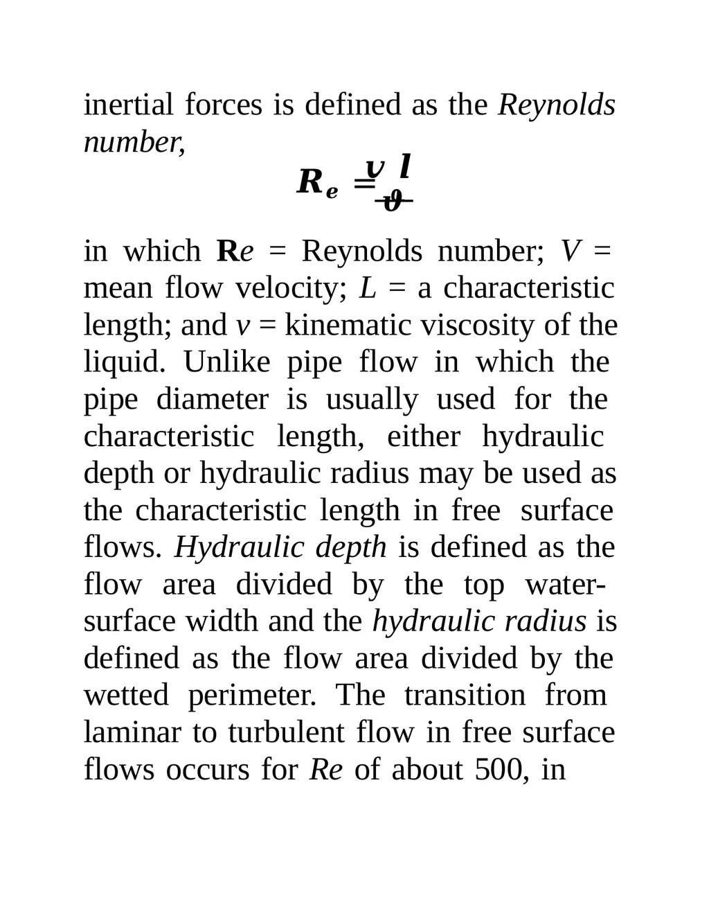
slide11. inertial forces is defined as the Reynolds number,
𝒗 𝒍
𝑹𝒆 = 𝝑
in which Re = Reynolds number; V = mean flow velocity; L = a characteristic length; and ν = kinematic viscosity of the liquid. Unlike pipe flow in which the pipe diameter is usually used for the characteristic length, either hydraulic depth or hydraulic radius may be used as the characteristic length in free surface flows. Hydraulic depth is defined as the flow area divided by the top water- surface width and the hydraulic radius is defined as the flow area divided by the wetted perimeter. The transition from laminar to turbulent flow in free surface flows occurs for Re of about 500, in<br>
slide12. which Re is based on the hydraulic radius as the characteristic length.
If Re< 500 or 600 laminar flow Re= 500-2000 transition flow Re>2000 turbulent
Subcritical, Supercritical, and Critical Flows
A flow is called critical if the flow
velocity is equal to the velocity of a gravity wave having small amplitude. A gravity wave may be produced by a change in the flow depth. The flow is called subcritical flow, if the flow velocity is less than the critical velocity, and the flow is called supercritical flow if the flow velocity is greater than the critical velocity. The Froude number, Fr, is equal to the ratio of inertial and gravitational forces and, for a rectangular channel, it is defined as<br>
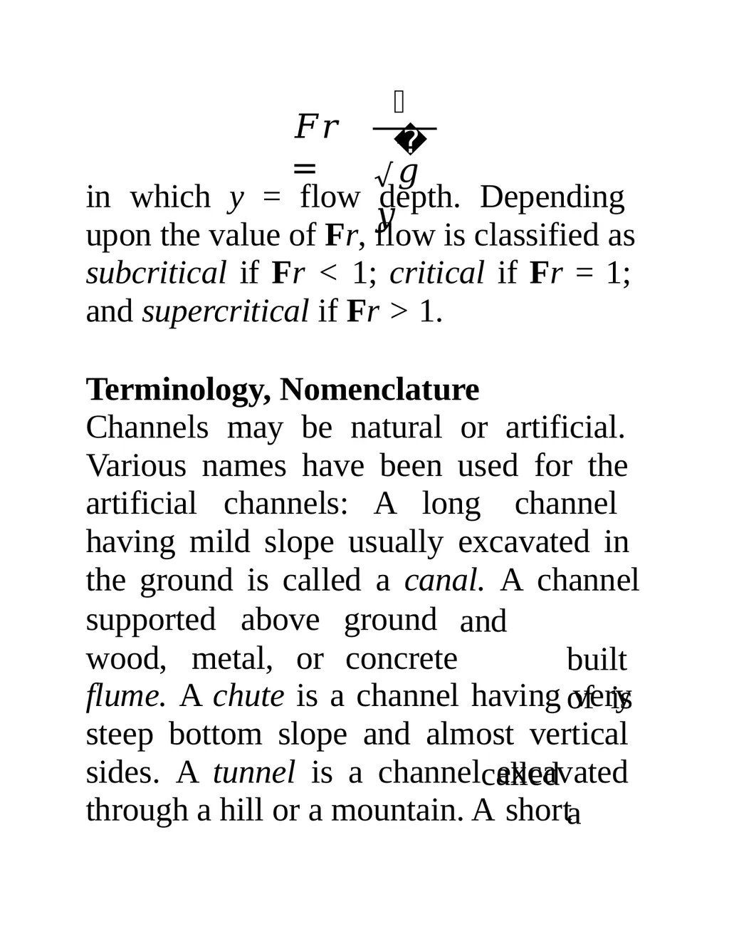
slide13. 𝐹𝑟 = 𝑉 √𝑔𝑦 in which y = flow depth. Depending upon the value of Fr, flow is classified as subcritical if Fr < 1; critical if Fr = 1; and supercritical if Fr > 1.

Terminology, Nomenclature
Channels may be natural or artificial. Various names have been used for the artificial channels: A long channel having mild slope usually excavated in the ground is called a canal. A channel wood, metal, or supported above ground
concrete and built of is called a flume. A chute is a channel having very steep bottom slope and almost vertical sides. A tunnel is a channel excavated through a hill or a mountain. A short<br>
slide14. channel flowing partly full is referred to as a culvert.
A channel having the same cross section and bottom slope throughout is referred to as a prismatic channel, whereas a
channel having varying cross section and/or bottom slope is called a non- prismatic channel. A long channel may be comprised of several prismatic
channels. A cross section taken normal to
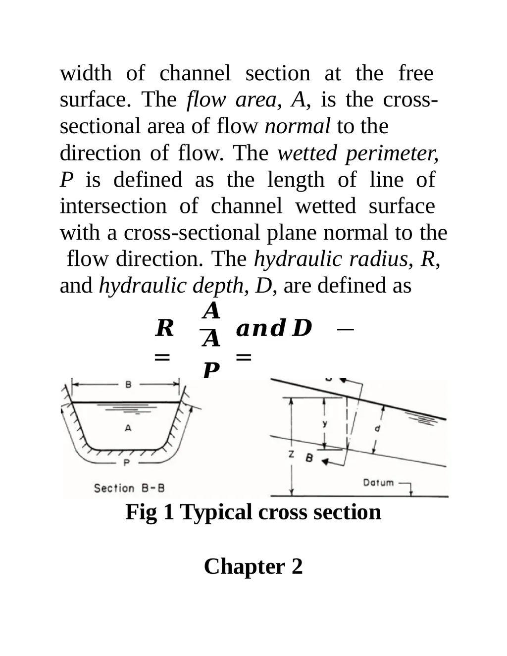
the direction of flow (e.g., Section BB in Fig. 1) is called a channel section. The depth of flow, y, at a section is the vertical distance of the lowest point of the channel section from the free surface. The depth of flow section, d, is the depth of flow normal to the direction of flow. The stage, Z, is the elevation or vertical distance of free surface above a specified datum ( Fig.1). The top width, B, is the<br>
slide15. width of channel section at the free surface. The flow area, A, is the cross- sectional area of flow normal to the direction of flow. The wetted perimeter, P is defined as the length of line of intersection of channel wetted surface with a cross-sectional plane normal to the flow direction. The hydraulic radius, R, and hydraulic depth, D, are defined as 𝑹 = 𝒂𝒏𝒅 𝑫 = 𝑨 𝑨
𝑷 𝑩 Fig 1 Typical cross section

Chapter 2<br>
slide16. Velocity and Pressure Distribution
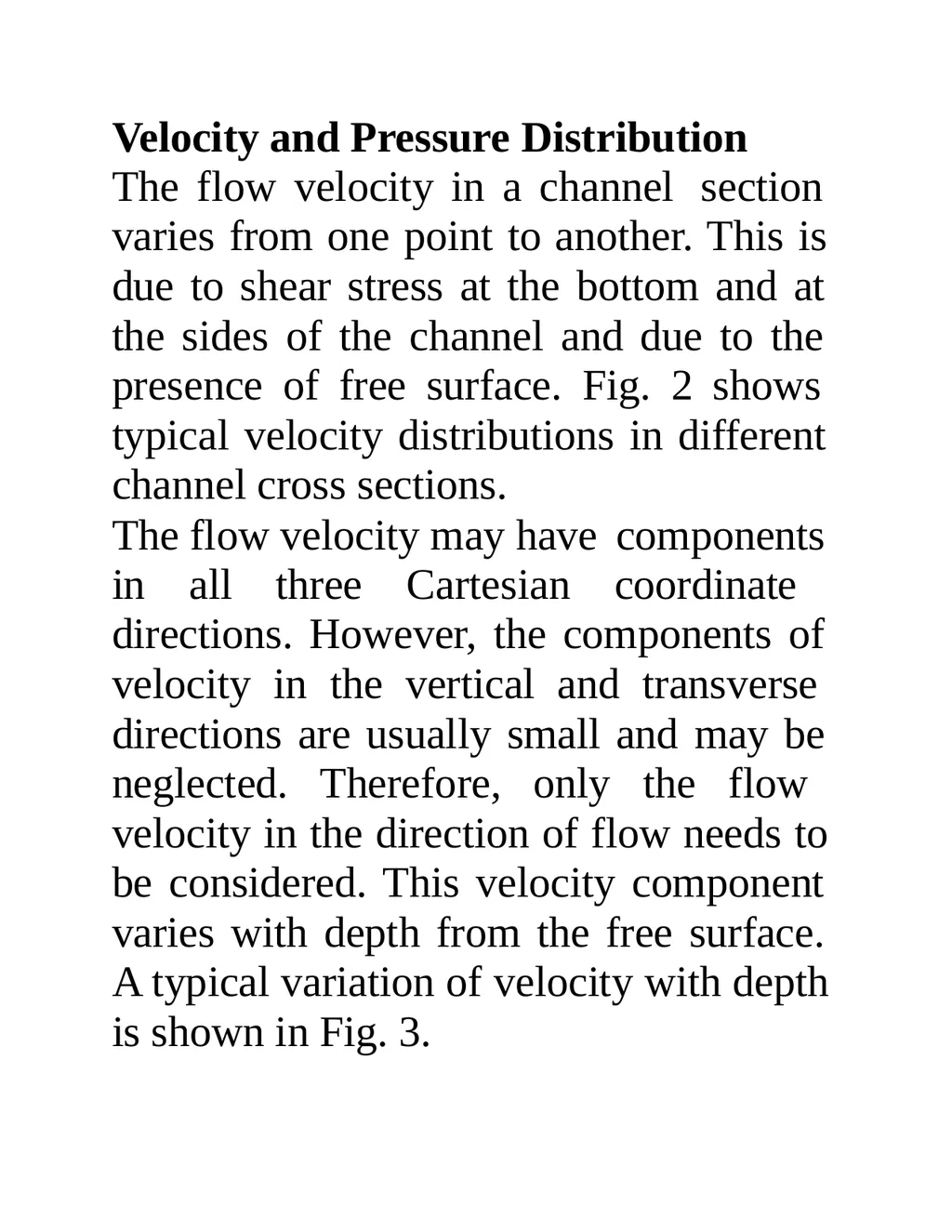
The flow velocity in a channel section varies from one point to another. This is due to shear stress at the bottom and at the sides of the channel and due to the presence of free surface. Fig. 2 shows typical velocity distributions in different channel cross sections.
The flow velocity may have components
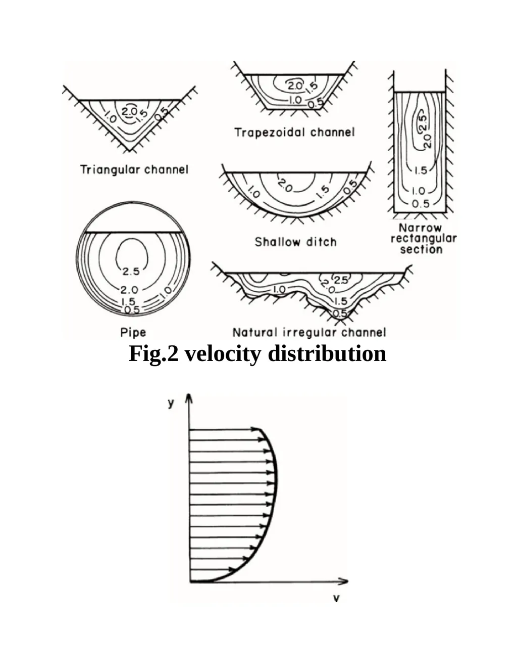
in all three Cartesian coordinate directions. However, the components of velocity in the vertical and transverse directions are usually small and may be neglected. Therefore, only the flow velocity in the direction of flow needs to be considered. This velocity component varies with depth from the free surface. A typical variation of velocity with depth is shown in Fig. 3.<br>
slide17. Fig.2 velocity distribution<br>
slide18. Fig. 3 Typical velocity variation with depth
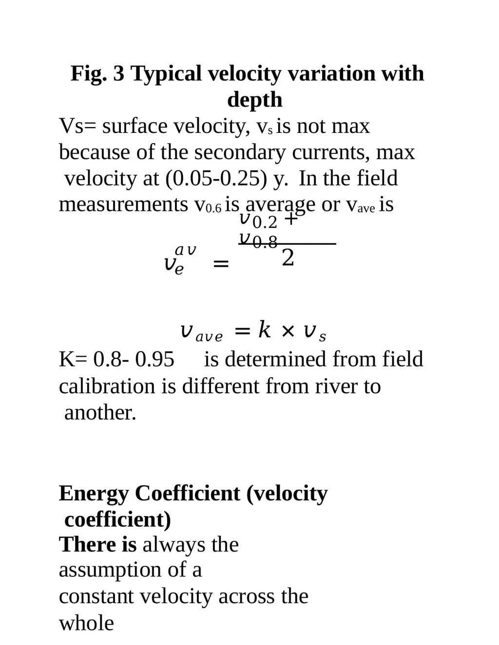
Vs= surface velocity, vs is not max because of the secondary currents, max velocity at (0.05-0.25) y. In the field measurements v0.6 is average or vave is 𝑎𝑣𝑒 𝑣0.2 + 𝑣0.8
𝑣 = 2 K= 0.8- 0.95 𝑣𝑎𝑣𝑒 = 𝑘 × 𝑣𝑠
is determined from field calibration is different from river to another.

Energy Coefficient (velocity coefficient)
There is always the assumption of a
constant velocity across the whole<br>
slide19. section of the flows but this is never true in practice because viscous drag makes the velocity lower near the solid boundaries.
As discussed in the previous paragraphs,
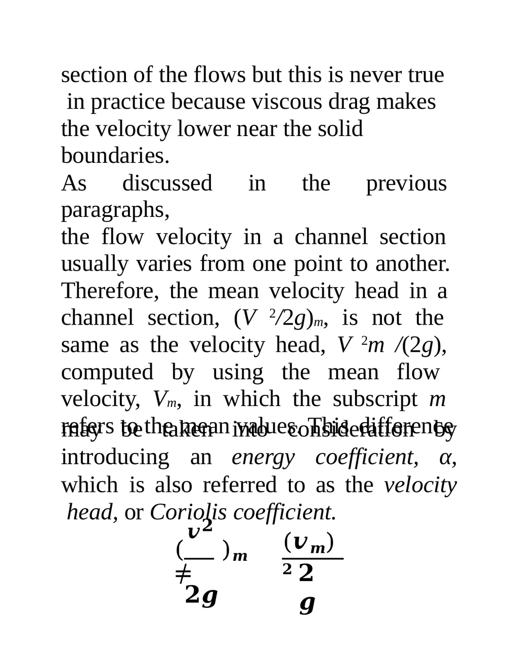
the flow velocity in a channel section usually varies from one point to another. Therefore, the mean velocity head in a channel section, (V 2/2g)m, is not the same as the velocity head, V 2m /(2g), computed by using the mean flow velocity, Vm, in which the subscript m refers to the mean values. This difference introducing an energy coefficient, may be taken into consideration by
α, which is also referred to as the velocity head, or Coriolis coefficient. 𝒗𝟐
( )𝒎 ≠
𝟐𝒈 (𝒗𝒎)𝟐 𝟐𝒈<br>
slide20. (v2/2g)m true mean velocity head BASIC CONCEPTS
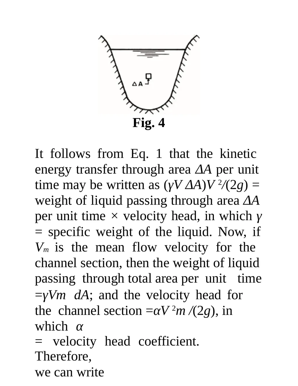
Referring to Fig. 4, the mass of liquid flowing through area ΔA per unit time = ρV ΔA, in which ρ = mass density of the liquid. Since, the kinetic energy of mass m traveling at velocity V is (1/2)mV 2, we can write
Kinetic energy transfer through area ΔA
per unit time 𝟐 𝟏 𝟐 𝟑 = 𝝆 𝑽 ∆ 𝑨 = 𝟏 𝝆 𝑽 ∆ 𝑨𝑽𝟐 (1)
(1) Kinetic energy transfer through area A
per unit time 𝟏 𝟐 𝟑 = 𝝆 ∫ 𝑽 𝑨 (2)<br>
slide21. Fig. 4 It follows from Eq. 1 that the kinetic energy transfer through area ΔA per unit time may be written as (γV ΔA)V 2/(2g) = weight of liquid passing through area ΔA per unit time × velocity head, in which γ
= specific weight of the liquid. Now, if
Vm is the mean flow velocity for the channel section, then the weight of liquid passing through total area per unit time
=γVm dA; and the velocity head for the channel section =αV 2m /(2g), in which α
= velocity head coefficient. Therefore,
we can write<br>
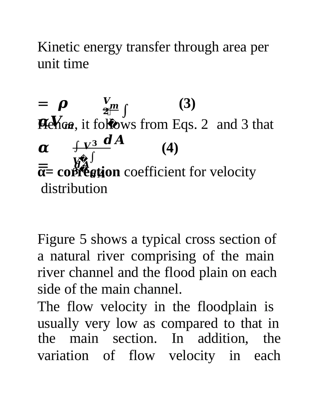
slide22. Kinetic energy transfer through area per unit time = 𝝆 𝜶𝑽𝒎 𝑽𝟐 𝟐 𝒎 ∫ 𝒅𝑨 (3) Hence, it follows from Eqs. 2 and 3 that 𝜶 = ∫ 𝑽𝟑 𝒅𝑨 𝒎 𝑽𝟑 ∫ 𝒅𝑨 (4) α= correction coefficient for velocity distribution

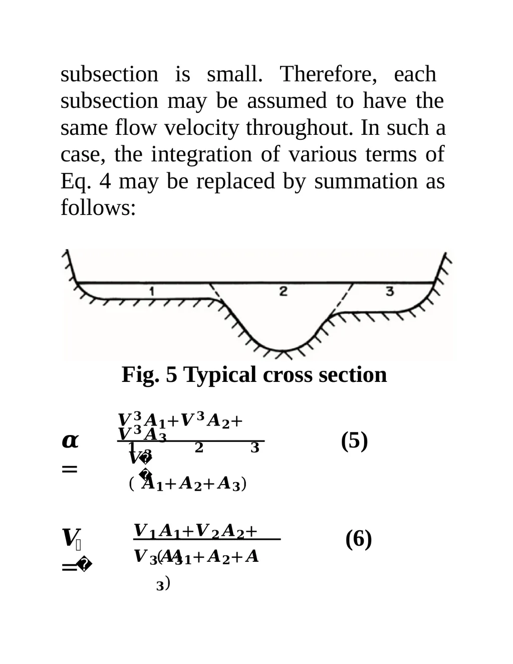
Figure 5 shows a typical cross section of a natural river comprising of the main river channel and the flood plain on each side of the main channel.
The flow velocity in the floodplain is usually very low as compared to that in variation of flow velocity in the main section. In addition, the
each<br>
slide23. subsection is small. Therefore, each subsection may be assumed to have the same flow velocity throughout. In such a case, the integration of various terms of Eq. 4 may be replaced by summation as follows: Fig. 5 Typical cross section 𝜶 = 𝑽𝟑𝑨𝟏+𝑽𝟑𝑨𝟐+ 𝑽𝟑𝑨𝟑
𝟏 𝟐 𝟑 𝒎 𝑽𝟑 ( 𝑨𝟏+𝑨𝟐+𝑨𝟑) (5) 𝒎 𝑽 = 𝑽𝟏𝑨𝟏+𝑽𝟐𝑨𝟐+ 𝑽𝟑𝑨𝟑 ( 𝑨𝟏+𝑨𝟐+𝑨𝟑) (6)<br>
slide24. By substituting Eq. 6 into Eq. 5 and simplifying, we obtain (𝑽𝟑𝑨𝟏+𝑽𝟑𝑨𝟐+ 𝑽𝟑𝑨𝟑) (𝑨𝟏+𝑨𝟐+𝑨𝟑)𝟐
𝟏 𝟐 𝟑
(𝑽𝟏𝑨𝟏+𝑽𝟐𝑨𝟐+𝑽𝟑𝑨𝟑) 𝟑 𝜶 =
(7) Note that Eq. 7 is written for a section which may be divided into three subsections each having uniform velocity distribution. For a general case in which total area A may be subdivided into N such subareas each having uniform velocity, an equation similar to Eq. 7 may be written as 𝜶 = ∑𝑵 (𝑽𝟑𝑨𝒊) .(∑ 𝑨𝒊)𝟐 𝒊=𝟏 𝒊
(∑ 𝑽𝒊𝑨𝒊) 𝟑 (8) Momentum Coefficient<br>
slide25. Similar to the energy coefficient, a coefficient for the momentum transfer through a channel section may be introduced to account for non uniform velocity distribution. This coefficient, also called Boussinesq coefficient, is denoted by β. An expression for this may be obtained as follows:

BASIC CONCEPTS
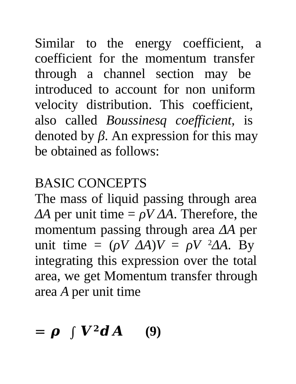
The mass of liquid passing through area ΔA per unit time = ρV ΔA. Therefore, the momentum passing through area ΔA per unit time = (ρV ΔA)V = ρV 2ΔA. By integrating this expression over the total area, we get Momentum transfer through area A per unit time

= 𝝆 ∫ 𝑽𝟐𝒅𝑨 (9)<br>
slide26. By introducing the momentum coefficient, β, we may write the momentum transfer through area A in terms of the mean flow velocity, Vm, for the channel section, i.e.,
Momentum transfer through area A per unit time = 𝜷𝝆 𝑽𝟐 ∫ 𝒅𝑨 (10)
𝒎

Hence, it follows from Eqs. 9 and 10 that 𝜷 = ∫ 𝑽𝟐𝒅𝑨 𝒎 𝑽𝟐 ∫ 𝒅𝑨 (11) Theoretical values for α and β can be derived from the power law and the logarithmic law for velocity distribution in wide channels. For turbulent flow in a straight channel having a rectangular, trapezoidal, or circular cross section, α is<br>
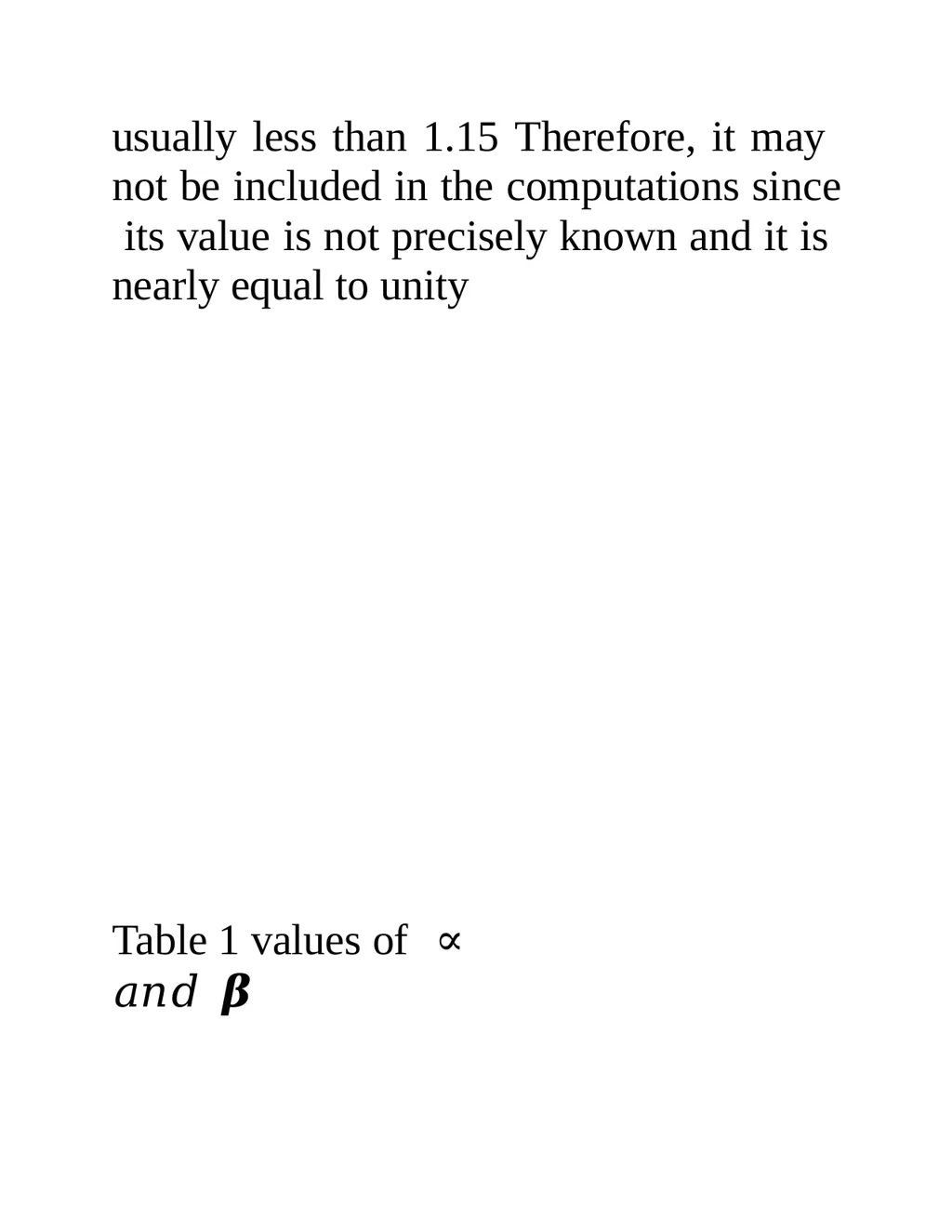
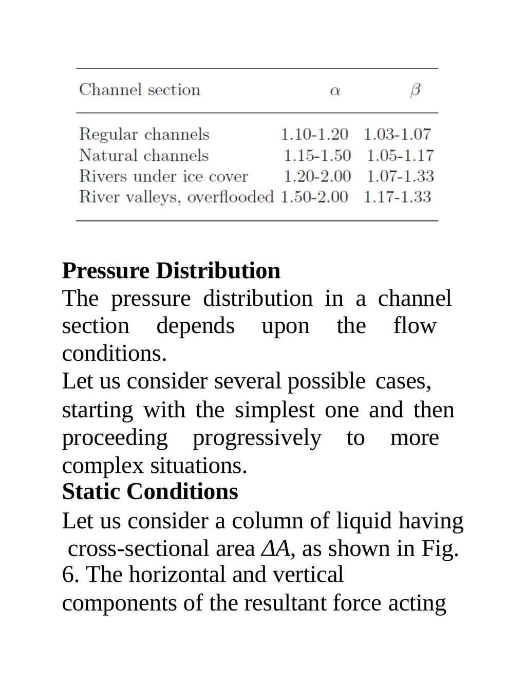
slide27. usually less than 1.15 Therefore, it may not be included in the computations since its value is not precisely known and it is nearly equal to unity Table 1 values of ∝ 𝑎𝑛𝑑 𝜷<br>
slide28. Pressure Distribution
The pressure distribution in a channel section depends upon the flow conditions.
Let us consider several possible cases,
starting with the simplest one and then proceeding progressively to more complex situations.
Static Conditions
Let us consider a column of liquid having cross-sectional area ΔA, as shown in Fig.
6. The horizontal and vertical
components of the resultant force acting<br>
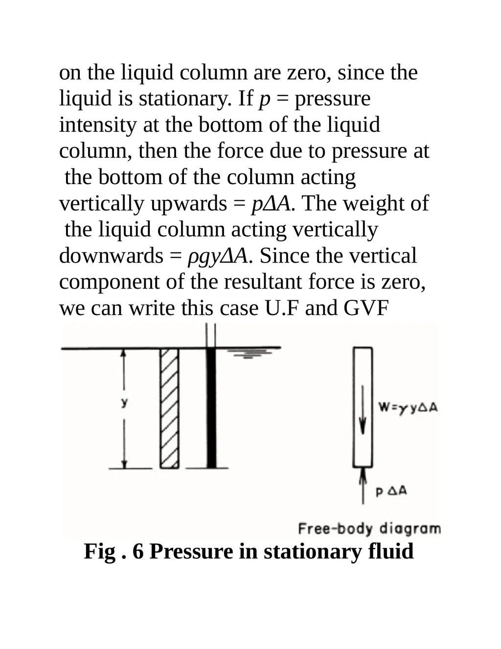
slide29. on the liquid column are zero, since the liquid is stationary. If p = pressure intensity at the bottom of the liquid column, then the force due to pressure at the bottom of the column acting vertically upwards = pΔA. The weight of the liquid column acting vertically downwards = ρgyΔA. Since the vertical component of the resultant force is zero, we can write this case U.F and GVF Fig . 6 Pressure in stationary fluid<br>
slide30. 𝒑 ∆𝑨 = 𝝆𝒈 𝒚 ∆ 𝑨

𝒑 = 𝝆𝒈 𝒚
In other words, the pressure intensity is directly proportional to the depth below the free surface. Since ρ is constant for typical engineering applications, the relationship between the pressure intensity and depth plots as a straight line, and the liquid rises to the level of the free surface in a piezometer, as shown in Fig. 6. The linear relationship, based on the assumption that ρ is constant, is usually valid except at very large depths, where large pressures result in increased density.

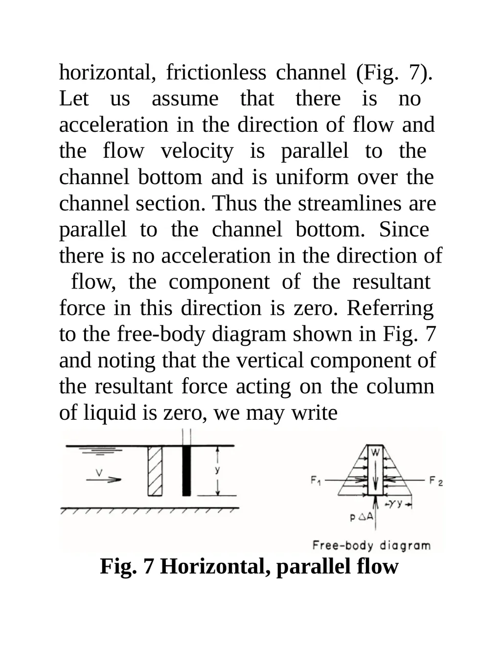
Horizontal, Parallel Flow
Let us now consider the forces acting on a vertical column of liquid flowing in a<br>
slide31. horizontal, frictionless channel (Fig. 7). Let us assume that there is no acceleration in the direction of flow and the flow velocity is parallel to the channel bottom and is uniform over the channel section. Thus the streamlines are parallel to the channel bottom. Since there is no acceleration in the direction of flow, the component of the resultant force in this direction is zero. Referring to the free-body diagram shown in Fig. 7 and noting that the vertical component of the resultant force acting on the column of liquid is zero, we may write Fig. 7 Horizontal, parallel flow<br>
slide32. 𝒑 𝒈 𝒚∆𝑨 = 𝝆 ∆ 𝑨

𝒑 = 𝝆𝒈 𝒚 = 𝜸 𝒚
in which γ = ρg = specific weight of the liquid. Note that this pressure distribution is the same as if the liquid were stationary; it is, therefore, referred to as the hydrostatic pressure distribution

Parallel Flow in Sloping Channels
Let us now consider the flow conditions in a sloping channel such that there is no acceleration in the flow direction, the flow velocity is uniform at a channel cross section and is parallel to the channel bottom; i.e., the streamlines are parallel to the channel bottom. Figure 8 shows the free-body diagram of a column of liquid normal to the channel bottom.
The cross-sectional area of the column is<br>
slide33. ΔA. If θ = slope of the channel bottom, then the component of the weight of column acting along the column is ρgdΔAcos θ and the force acting at the bottom of the column is pΔA. There is no acceleration in a direction along the column length, since the flow velocity is parallel to the channel bottom. Fig. 8 Parallel flow in a sloping channel

Hence, we can write pΔA = ρgdΔAcos θ, or p = ρgd cos θ = γd cos θ.
By substituting d = y cos θ into this
equation (y = flow depth measured vertically, as shown in Fig. 8, we obtain<br>
slide34. 𝒑 = 𝝆𝒈 𝒚 = 𝜸 𝒚𝒄𝒐𝒔 𝜽𝟐
Note that in this case the pressure distribution is not hydrostatic in spite of the fact that we have parallel flow and there is no acceleration in the direction of flow. However, if the slope of the channel bottom is small, then cos θ _ 1 and d _ y. Hence,
𝒑 ≅ 𝝆𝒈 𝒅 ≅ 𝝆𝒈 𝒚
In several derivations we assume that the slope of the channel bottom is small. With this assumption, the pressure distribution may be assumed to be hydrostatic if the streamlines are almost parallel and straight, and the flow depths measured vertically or normal to the channel bottom are approximately the same.<br>
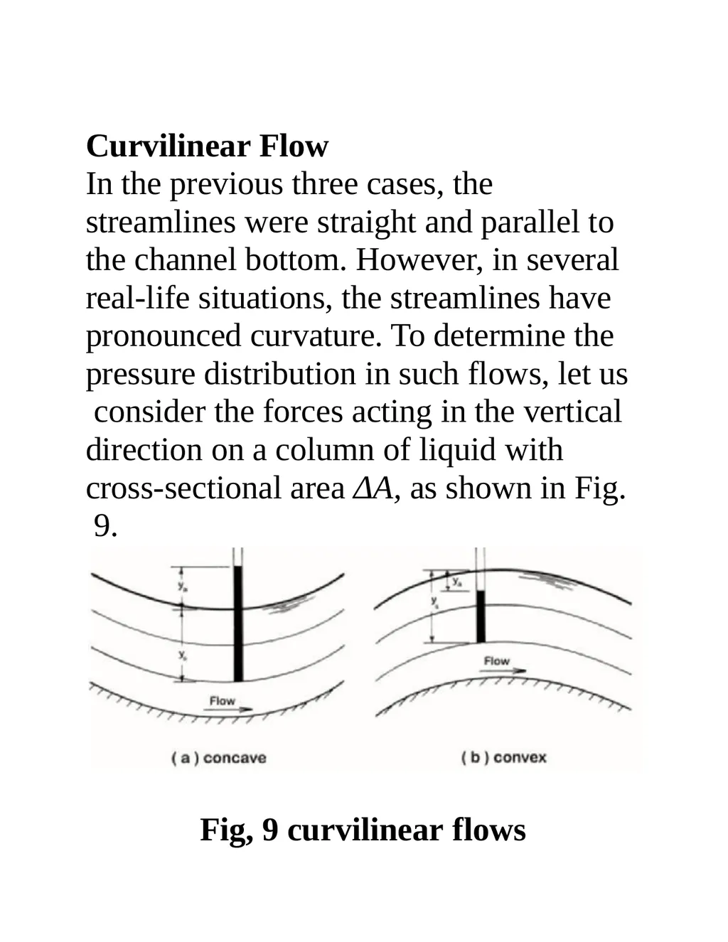
slide35. Curvilinear Flow
In the previous three cases, the streamlines were straight and parallel to the channel bottom. However, in several real-life situations, the streamlines have pronounced curvature. To determine the pressure distribution in such flows, let us consider the forces acting in the vertical direction on a column of liquid with cross-sectional area ΔA, as shown in Fig. 9. Fig, 9 curvilinear flows<br>
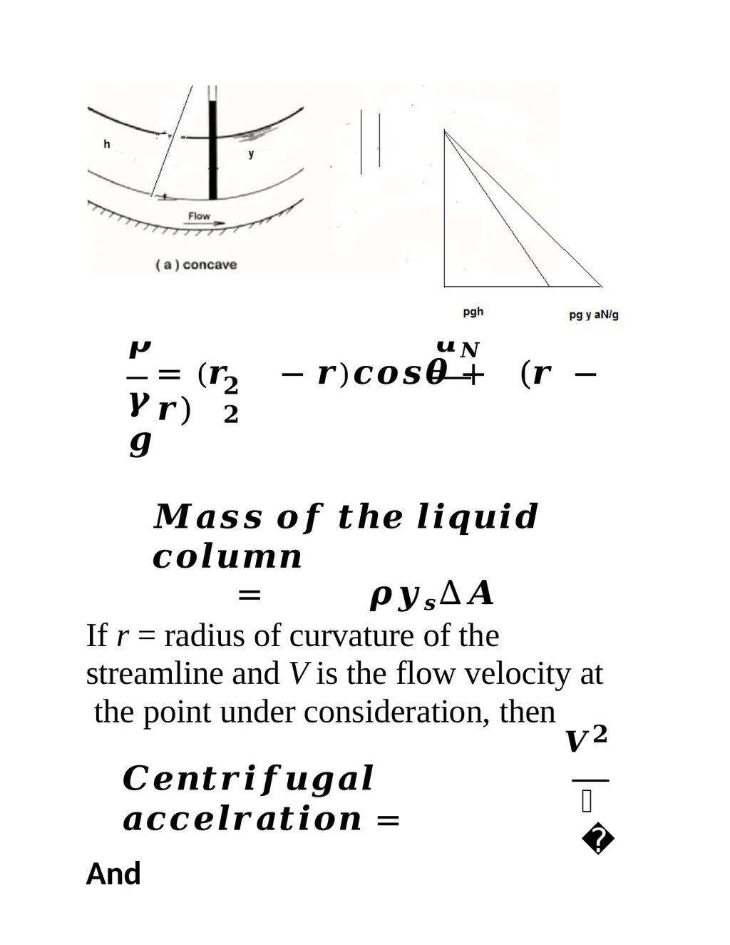
slide36. 𝜸 𝒈 𝟐 𝟐 𝒑 𝒂𝑵
= (𝒓 − 𝒓)𝒄𝒐𝒔𝜽 + (𝒓 − 𝒓) 𝑴𝒂𝒔𝒔 𝒐𝒇 𝒕𝒉𝒆 𝒍𝒊𝒒𝒖𝒊𝒅 𝒄𝒐𝒍𝒖𝒎𝒏
= 𝝆𝒚𝒔∆𝑨 If r = radius of curvature of the streamline and V is the flow velocity at the point under consideration, then
𝑽𝟐 𝒓 𝑪𝒆𝒏𝒕𝒓𝒊𝒇𝒖𝒈𝒂𝒍 𝒂𝒄𝒄𝒆𝒍𝒓𝒂𝒕𝒊𝒐𝒏 =
And<br>
slide37. 𝑪𝒆𝒏𝒕𝒓𝒊𝒇𝒖𝒈𝒂𝒍 𝒇𝒐𝒓𝒄𝒆 = 𝝆𝒚𝒔∆𝑨 𝑽𝟐 𝒓 Dividing the centrifugal force by the area of the column and converting the pressure to pressure head, we obtain the following expression for the pressure head, ya, acting at the bottom of the liquid column due to centrifugal acceleration 𝟏
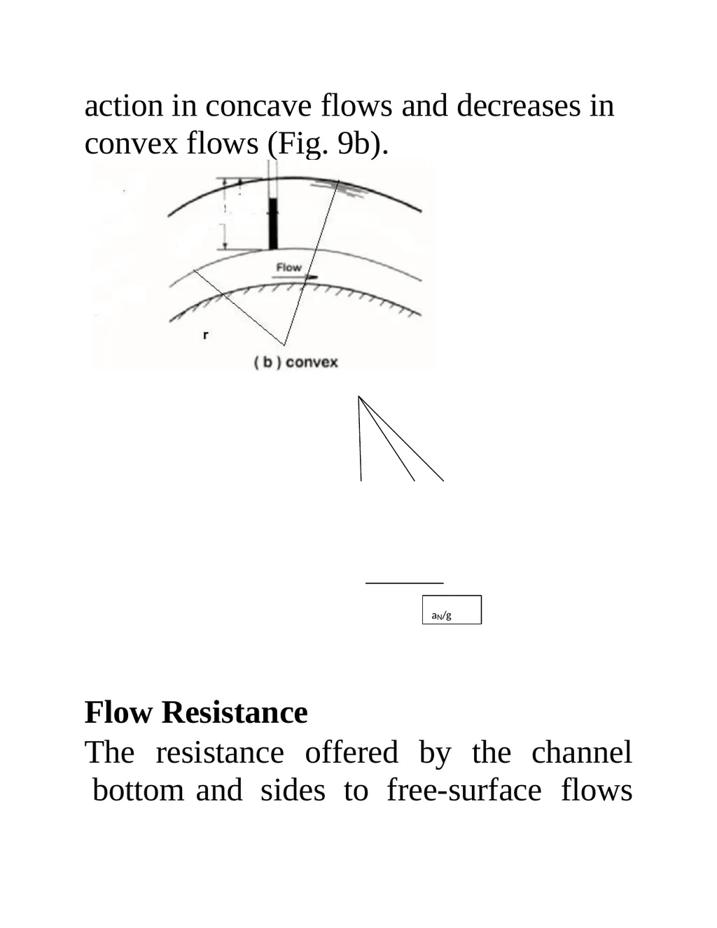
𝒚𝒂 = 𝒈 𝒚𝒔 𝑽𝟐 𝒓 The pressure due to centrifugal force is in the same direction as the weight of column if the curvature is concave, as shown in Fig. 9 a, and it is in a direction opposite to the weight if the curvature is convex (Fig. 9b). Therefore, the total<br>
slide38. pressure head acting at the bottom of the column is an algebraic sum of the pressure due to centrifugal action and the weight of the liquid column, i.e., 𝒔 𝑻𝒐𝒕𝒂𝒍 𝒑𝒓𝒆𝒔𝒔𝒖𝒓𝒆 𝒉𝒆𝒂𝒅 = 𝒚 (𝟏 ∓ 𝟏 𝑽 𝟐 𝒈 𝒓 ) ( a)

A positive sign is used if the streamline is concave, and a negative sign is used if the streamline is convex. Note that the first term in Eq. a is the pressure head due to static conditions while the second term is the pressure head due to centrifugal action. Thus, the liquid in a piezometer inserted into the flow rises, as shown in Fig. 9a. In other words, pressure increases due to centrifugal<br>
slide39. action in concave flows and decreases in convex flows (Fig. 9b). Flow Resistance
The resistance offered by the channel bottom and sides to free-surface flows aN/g<br>
slide40. and its effects on the velocity distribution in an excellent manner as follows :
“The water of straight rivers is the swifter the farther away it is from the walls, because of resistance. Water has
higher speed on the surface than at the bottom. This happens because water on the surface borders on air which is of little resistance, because lighter than
water, and the water at the bottom is
touching the earth which is of higher resistance, because heavier than water and not moving. From this follows that the part which is more distant from the bottom has less resistance than that below. Because of the variation in resistance along the wetted perimeter and because of the shape of the channel cross section, secondary currents are usually set up in free-surface flows even if the<br>
slide41. channel is straight. In addition, the shear resistance offered to flow at the channel boundaries is not uniform. However, to simplify the analysis, we will assume that the flow is one-dimensional – i.e., there are no secondary currents in the flow and the shear resistance to flow at the boundaries is uniform.
Flow Resistance Equations
In this section, we present several equations relating the channel resistance to various flow variables. For a general derivation, we first derive an equation for non uniform flow and then simplify it for uniform flow as a special case of non uniform flow.
Chezy Equation
To derive the Chezy equation, we make the following assumptions: The flow is<br>
slide42. steady; the slope of the channel bottom is small; and the channel is prismatic.
Let us consider a control volume of length Δx, as shown in Fig. 10. At the upstream side of this control volume, let
the distance be x, flow velocity be V , and the flow depth be y. Then, the values of these variables at the downstream side are x + Δx, V + (dV/dx)Δx, and y +
(dy/dx)Δx).
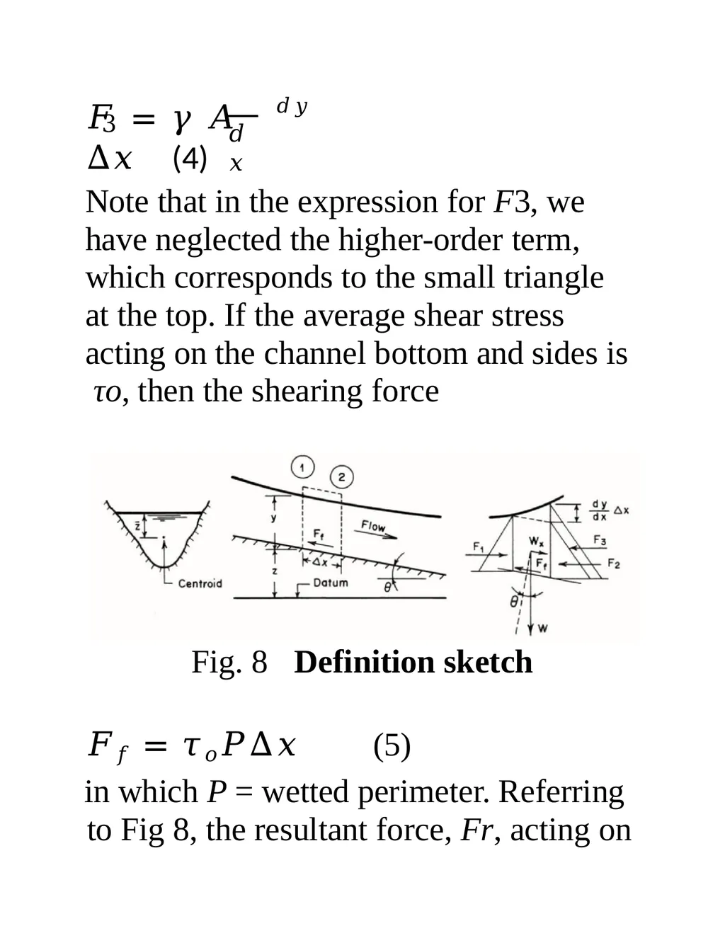
The following forces are acting on the control volume: pressure force on the upstream side, F1; pressure forces on the downstream side, F2 and F3; a component of the weight of water in the control volume in the downstream direction, Wx; and the shear force, Ff , acting on the channel bottom and the sides. Referring to Fig. 10, the expression<br>
slide43. for these forces may be written as follows

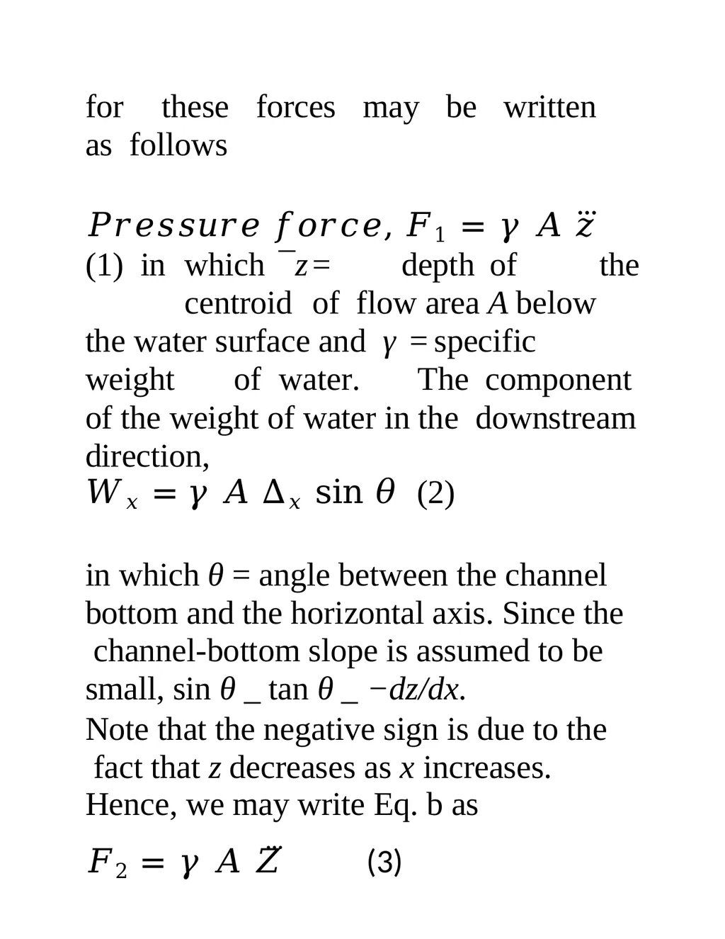
𝑃𝑟𝑒𝑠𝑠𝑢𝑟𝑒 𝑓𝑜𝑟𝑐𝑒, 𝐹1 = 𝛾 𝐴 𝑧⃛ (1) in which ¯z = depth of the centroid of flow area A below the water surface and γ = specific weight of water. The component of the weight of water in the downstream direction,
𝑊𝑥 = 𝛾 𝐴 ∆𝑥 sin 𝜃 (2)

in which θ = angle between the channel bottom and the horizontal axis. Since the channel-bottom slope is assumed to be small, sin θ _ tan θ _ −dz/dx.
Note that the negative sign is due to the fact that z decreases as x increases.
Hence, we may write Eq. b as
𝐹2 = 𝛾 𝐴 𝑍⃛ (3)<br>
slide44. 3 𝑑𝑥 𝐹 = 𝛾 𝐴 𝑑𝑦 ∆𝑥 (4) Note that in the expression for F3, we have neglected the higher-order term, which corresponds to the small triangle at the top. If the average shear stress acting on the channel bottom and sides is τo, then the shearing force Fig. 8 Definition sketch

𝐹𝑓 = 𝜏𝑜𝑃∆𝑥 (5)
in which P = wetted perimeter. Referring to Fig 8, the resultant force, Fr, acting on<br>
slide45. the control volume in the downstream direction is
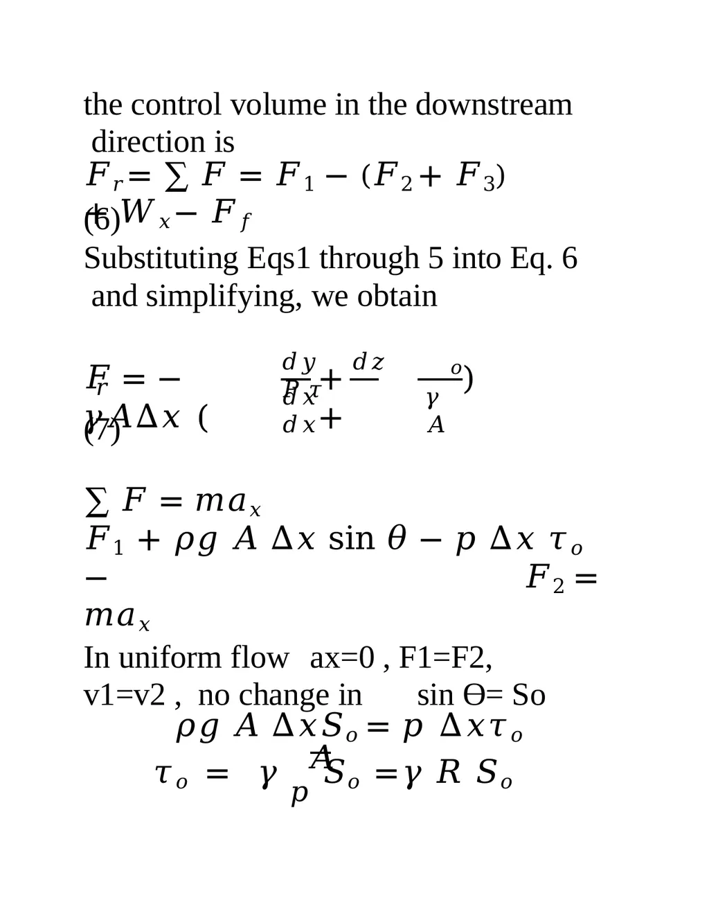
𝐹𝑟 = ∑ 𝐹 = 𝐹1 − (𝐹2 + 𝐹3) + 𝑊𝑥 − 𝐹𝑓 (6)
Substituting Eqs1 through 5 into Eq. 6 and simplifying, we obtain 𝐹 = − 𝛾𝐴∆𝑥 ( 𝑑𝑥 𝑑𝑥 + + 𝑑𝑦 𝑑𝑧 𝑃 𝜏 𝑜 𝛾 𝐴 ) 𝑟
(7) ∑ 𝐹 = 𝑚𝑎𝑥
𝐹1 + 𝜌𝑔 𝐴 ∆𝑥 sin 𝜃 − 𝑝 ∆𝑥 𝜏𝑜 − 𝐹2 =
𝑚𝑎𝑥
In uniform flow ax=0 , F1=F2, v1=v2 , no change in sin Ɵ= So
𝜌𝑔 𝐴 ∆𝑥𝑆𝑜 = 𝑝 ∆𝑥𝜏𝑜
𝐴
𝜏𝑜 = 𝛾 𝑝 𝑆𝑜 = 𝛾 𝑅 𝑆𝑜<br>
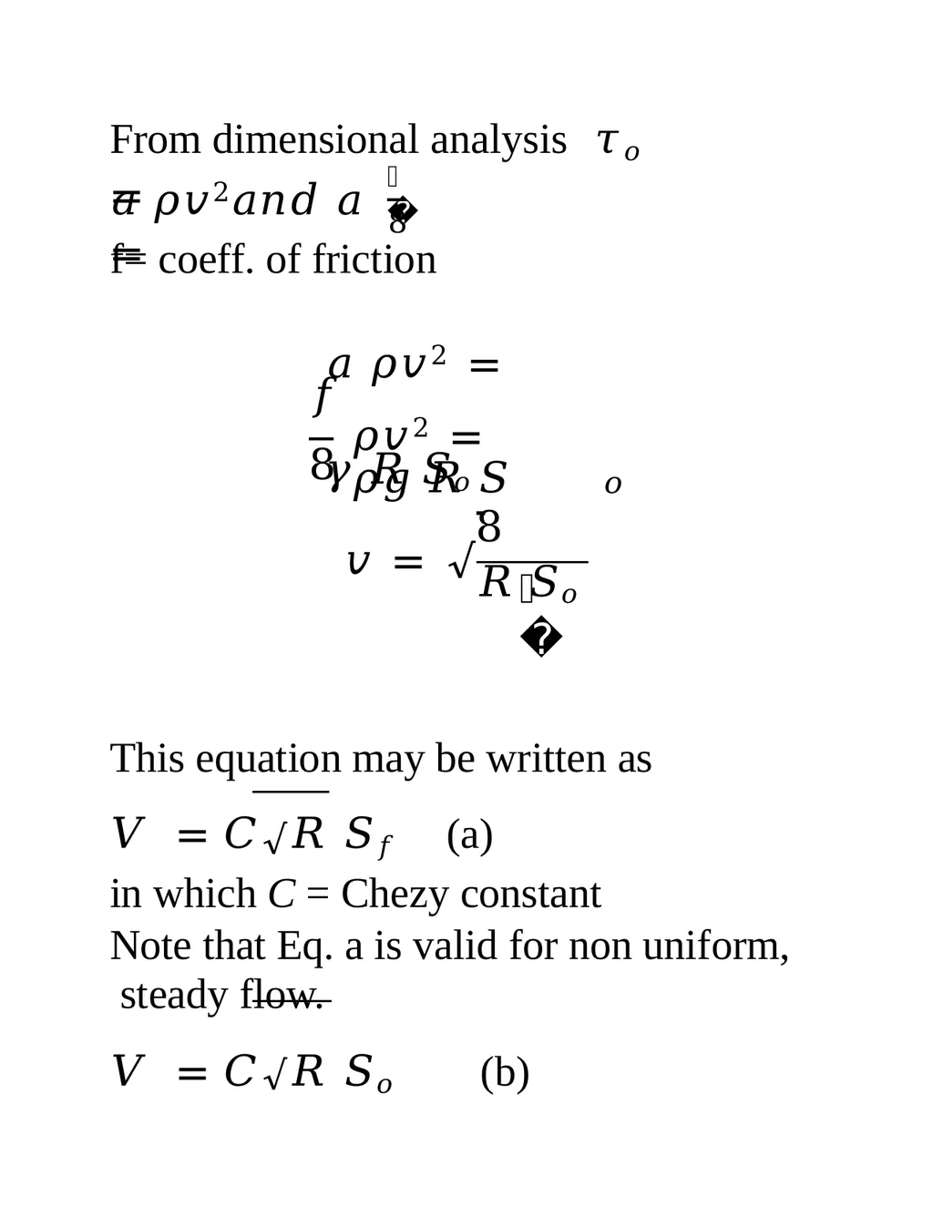
slide46. From dimensional analysis 𝜏𝑜 = 𝑎 𝜌𝑣2𝑎𝑛𝑑 𝑎 = 𝑓 8 f= coeff. of friction

𝑎 𝜌𝑣2 = 𝛾 𝑅 𝑆𝑜 8 𝑓
𝜌𝑣2 = 𝜌𝑔 𝑅 𝑆 𝑜 𝑣 = √ 8 𝑅 𝑆𝑜 𝑓 This equation may be written as
𝑉 = 𝐶√𝑅 𝑆𝑓 (a)
in which C = Chezy constant
Note that Eq. a is valid for non uniform, steady flow.
𝑉 = 𝐶√𝑅 𝑆𝑜 (b)<br>
slide47. For uniform flow we use Eqs b is valid. It is clear from Eq. a or b that C has dimensions of √ length/time, as compared to the Darcy Weisbach friction factor, f, which is dimensionless.
However, like f, C depends upon the channel roughness and the Reynolds number, Re. In addition, it may depend upon the channel cross-sectional shape as well, although this dependence appears to be small and may be neglected. Because the channel roughness may vary over a wide range, its effect on C has not been as thoroughly investigated as that on f.
Let us now compare the Chezy equation, Eq. a, for open channels with the Darcy- Weisbach friction formula for pipes,<br>
slide48. 𝐿 𝑣2
ℎ𝑓 = 𝑓 𝐷 2𝑔
in which hf = head loss in a pipe of diameter D and length L. The slope of the energy grade line, S = hf/L. Therefore, we may write this equation as 𝑉 = √ 2𝑔 𝐷 𝑆 𝑓 Noting that the hydraulic radius, R, for a pipe is equal to D/4, Eq. a
Becomes 𝐷 𝑆
𝑉 = 𝐶√ 4<br>
slide49. It follows from the above two equations that 8𝑔
𝐶 = √ 𝑓
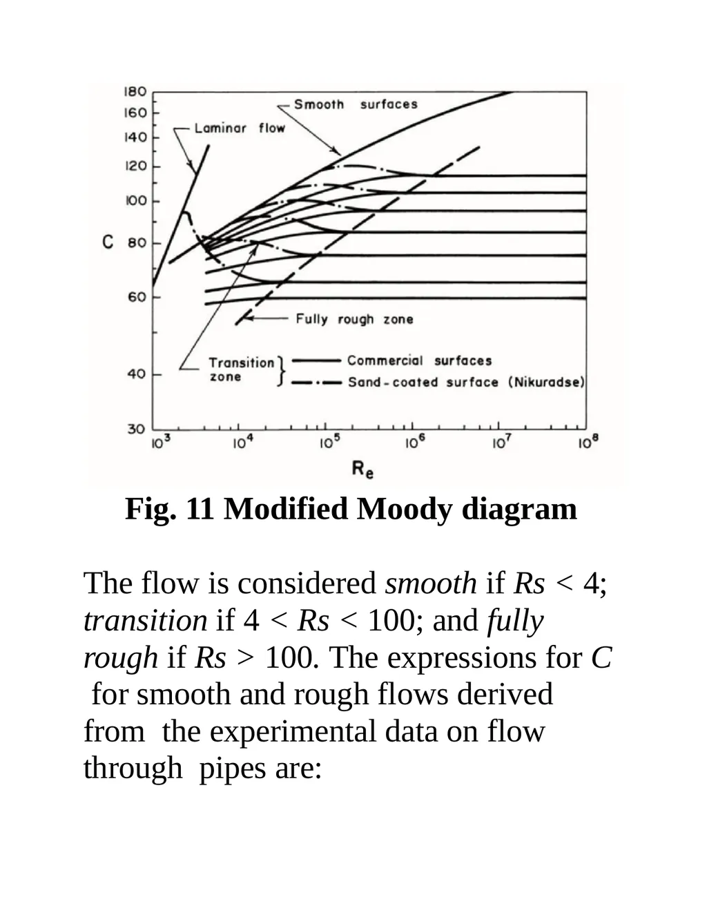
Figure 11 shows the Moody diagram plotted with C as the ordinate instead of f . This diagram is divided into three regions: hydraulically smooth, transition, and fully rough. A flow may be considered hydraulically smooth even though the channel surface is rough provided the projections of the surface roughness are covered by the laminar sublayer. increases, As the Reynolds number the thickness of this layer decreases and the effect of roughness projections on flow becomes important. Then, the flow is in the transition region. However, when the roughness projections are not covered by the<br>
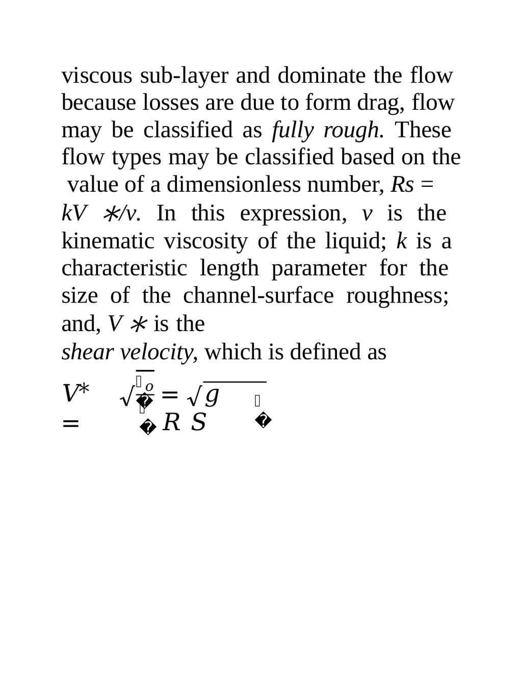
slide50. viscous sub-layer and dominate the flow because losses are due to form drag, flow may be classified as fully rough. These flow types may be classified based on the value of a dimensionless number, Rs = kV ∗/ν. In this expression, ν is the kinematic viscosity of the liquid; k is a characteristic length parameter for the size of the channel-surface roughness; and, V ∗ is the
shear velocity, which is defined as ∗ 𝑉 = √ 𝜏 𝑜 𝜌 √ = 𝑔 𝑅 𝑆 𝑓<br>
slide51. Fig. 11 Modified Moody diagram

The flow is considered smooth if Rs < 4; transition if 4 < Rs < 100; and fully rough if Rs > 100. The expressions for C for smooth and rough flows derived from the experimental data on flow through pipes are:<br>
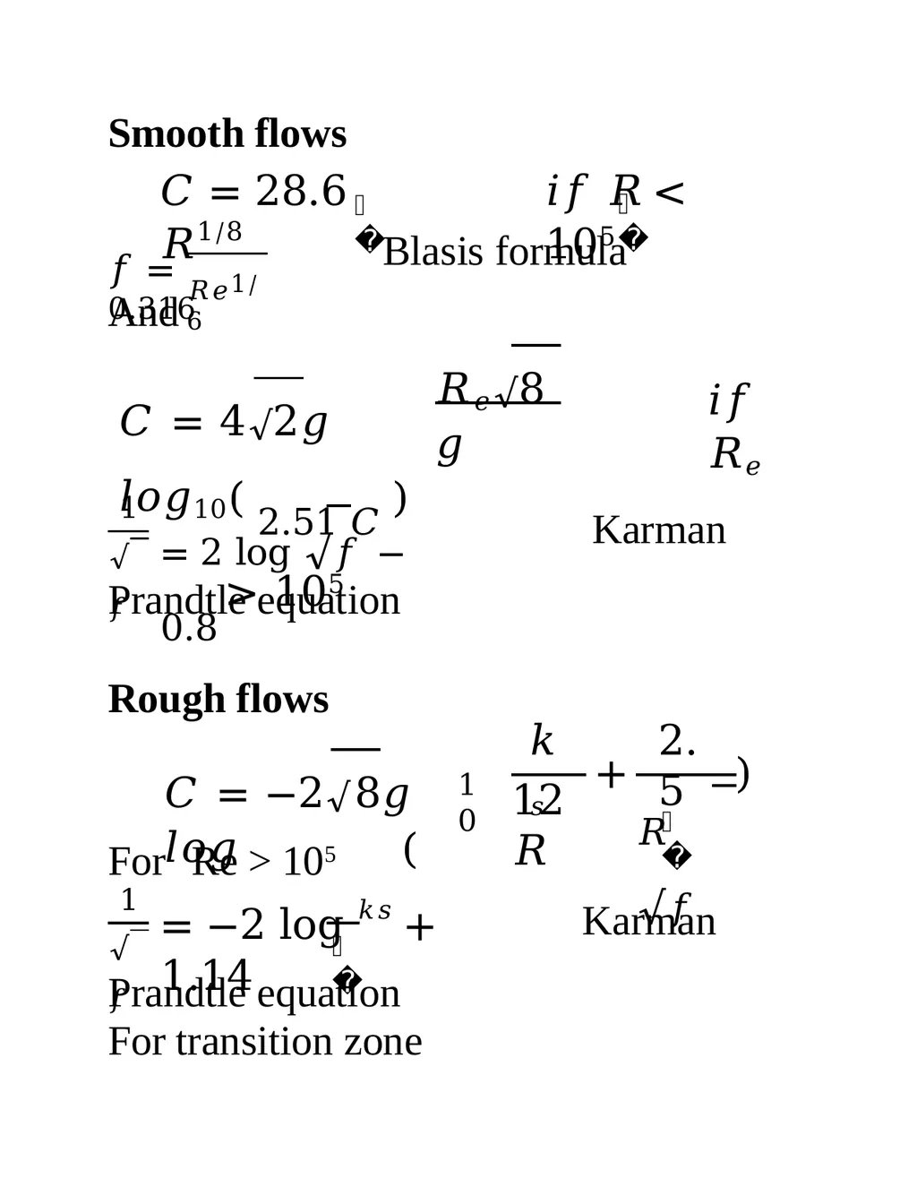
slide52. 𝑒 Smooth flows
𝐶 = 28.6 𝑅1/8 𝑒 𝑖𝑓 𝑅 < 105 𝑓 = 0.316 𝑅𝑒1/6 Blasis formula And 𝑅𝑒√8𝑔 𝑖𝑓 𝑅𝑒 𝐶 = 4√2𝑔 𝑙𝑜𝑔10( 2.51 𝐶 )
> 105 1 √𝑓 = 2 log √𝑓 − 0.8 Karman Prandtle equation

Rough flows 10 𝐶 = −2√8𝑔 𝑙𝑜𝑔 ( 𝑘𝑠 12𝑅 + 2.5 𝑒 𝑅 √𝑓 ) For Re > 105 1 √𝑓 𝐷 = −2 log 𝑘𝑠 + 1.14 Karman Prandtle equation For transition zone<br>
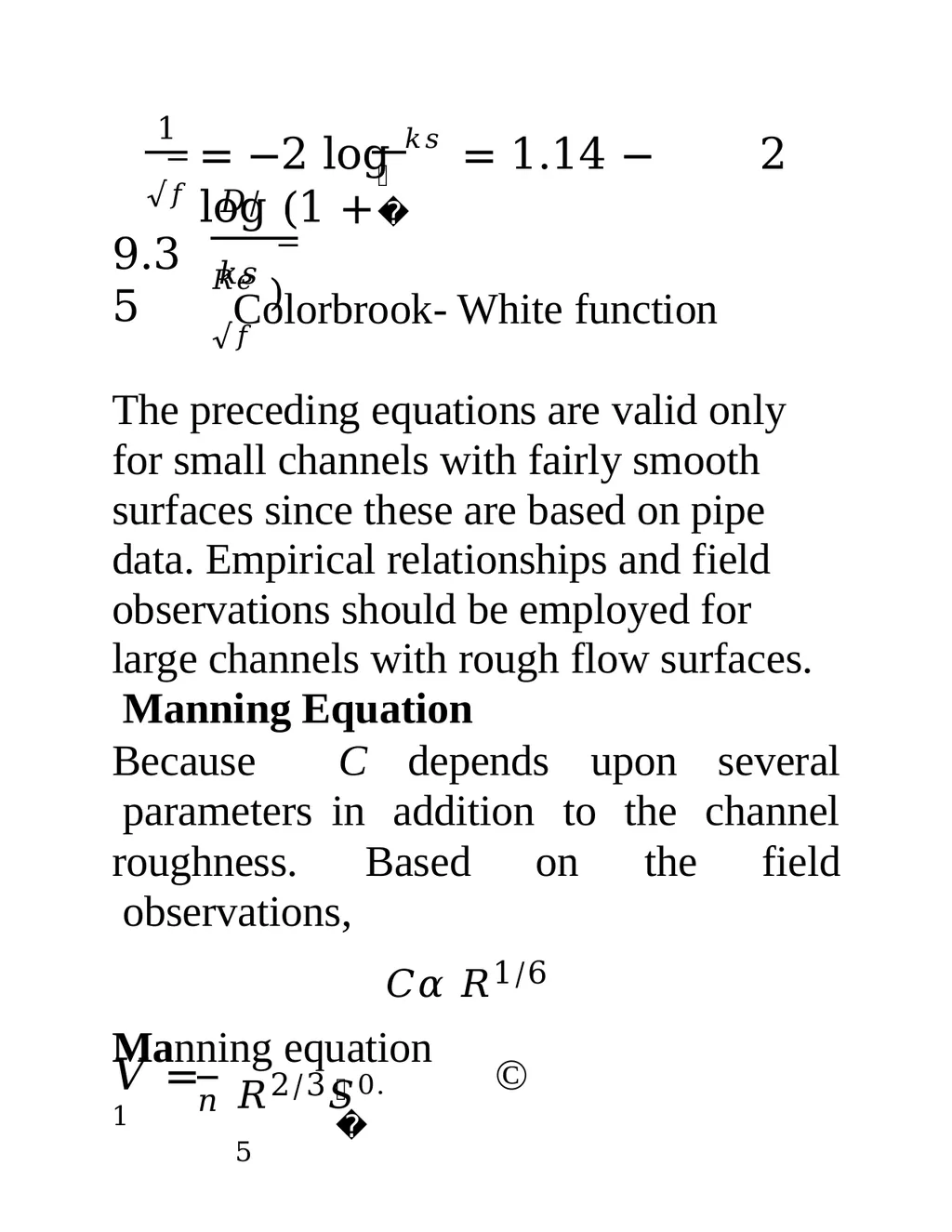
slide53. 1 𝐷 = −2 log 𝑘𝑠 = 1.14 − 2 log (1 + √𝑓
9.35 𝑅𝑒 √𝑓 𝐷/𝑘𝑠 ) Colorbrook- White function

The preceding equations are valid only for small channels with fairly smooth surfaces since these are based on pipe data. Empirical relationships and field observations should be employed for large channels with rough flow surfaces. Manning Equation
Because C depends upon several parameters in addition to the channel roughness. Based on the field observations, 𝐶𝛼 𝑅1/6
Manning equation 𝑉 = 1 𝑛 𝑓 𝑅2/3𝑆0.5 ©<br>
slide54. in which n = Manning coefficient. This is the Manning equation, which has been very widely used.
Again note that n is not a dimensionless constant and has the dimensions of (length)1/3/time.
The value of n depends mainly upon the
surface roughness, amount of vegetation, and channel irregularity, and, to a lesser degree, upon stage, scour and deposition, and channel alignment.
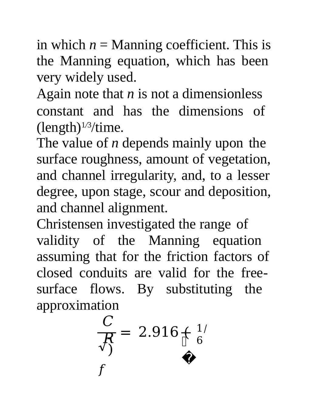
Christensen investigated the range of
validity of the Manning equation assuming that for the friction factors of closed conduits are valid for the free- surface flows. By substituting the approximation √𝑓 𝐶 𝑅 𝑘 = 2.916 ( ) 1/6<br>
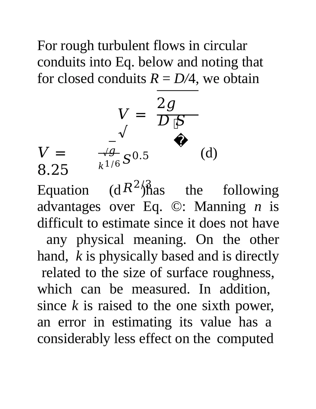
slide55. For rough turbulent flows in circular conduits into Eq. below and noting that for closed conduits R = D/4, we obtain 𝑉 = √ 2𝑔 𝐷 𝑆 𝑓 𝑉 = 8.25 √𝑔 𝑘1/6 𝑆0.5 𝑅2/3 (d) difficult to estimate since it does not have any physical meaning. On the other hand, k is physically based and is directly related to the size of surface roughness, which can be measured. In addition, since k is raised to the one sixth power, an error in estimating its value has a considerably less effect on the computed<br>
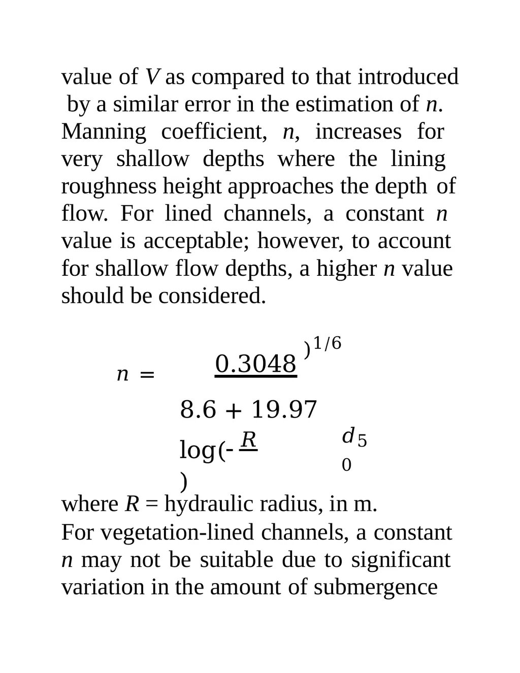
slide56. value of V as compared to that introduced by a similar error in the estimation of n.
Manning coefficient, n, increases for very shallow depths where the lining roughness height approaches the depth of
flow. For lined channels, a constant n value is acceptable; however, to account for shallow flow depths, a higher n value should be considered.
( 𝑅
)1/6
𝑛 = 0.3048 𝑑50 8.6 + 19.97 log( 𝑅 ) where R = hydraulic radius, in m.
For vegetation-lined channels, a constant n may not be suitable due to significant variation in the amount of submergence<br>
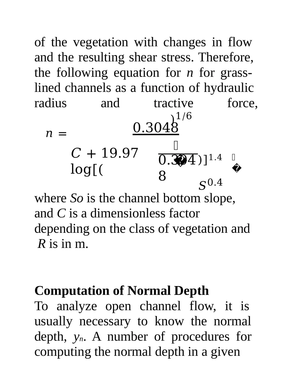
slide57. of the vegetation with changes in flow and the resulting shear stress. Therefore, the following equation for n for grass- lined channels as a function of hydraulic radius and tractive force, ( 𝑅
)1/6
𝑛 = 0.3048 𝐶 + 19.97 log[( 𝑅 0.3048 𝑜 )]1.4 𝑆0.4 where So is the channel bottom slope, and C is a dimensionless factor depending on the class of vegetation and R is in m.

Computation of Normal Depth
To analyze open channel flow, it is usually necessary to know the normal depth, yn. A number of procedures for computing the normal depth in a given<br>
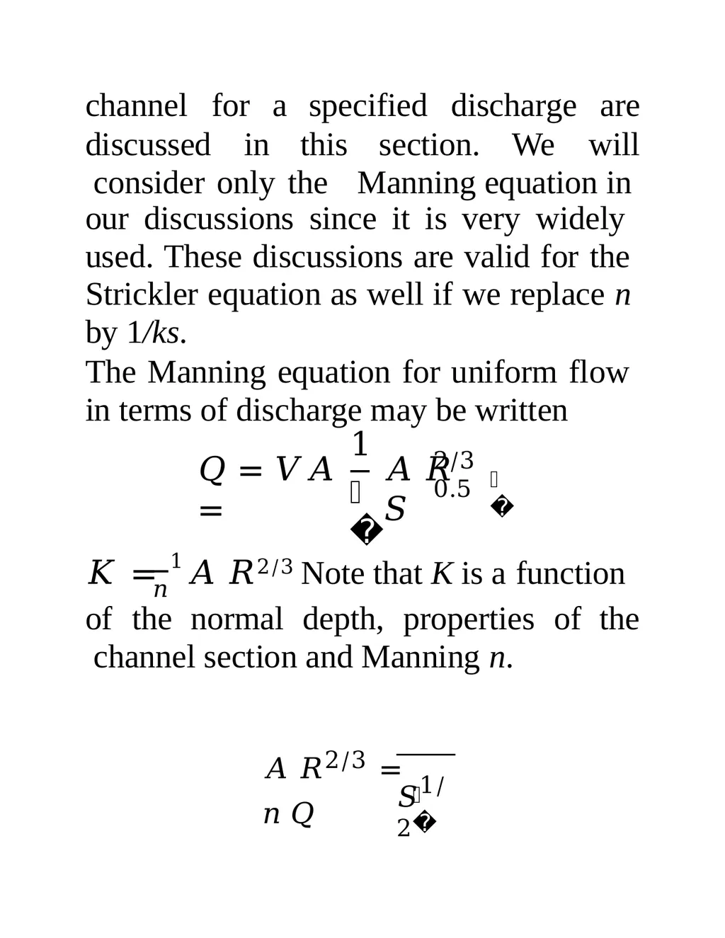
slide58. channel for a specified discharge are discussed in this section. We will consider only the Manning equation in our discussions since it is very widely used. These discussions are valid for the Strickler equation as well if we replace n by 1/ks.
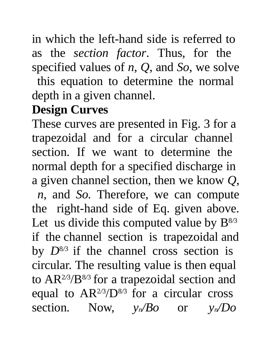
The Manning equation for uniform flow in terms of discharge may be written 𝑄 = 𝑉𝐴 = 1
𝑛 𝐴 𝑅 𝑆 𝑜 2/3 0.5 𝑛 𝐾 = 1 𝐴 𝑅2/3 Note that K is a function of the normal depth, properties of the channel section and Manning n. 𝐴 𝑅2/3 = 𝑛 𝑄 𝑜 𝑆1/2<br>
slide59. in which the left-hand side is referred to as the section factor. Thus, for the specified values of n, Q, and So, we solve this equation to determine the normal depth in a given channel.
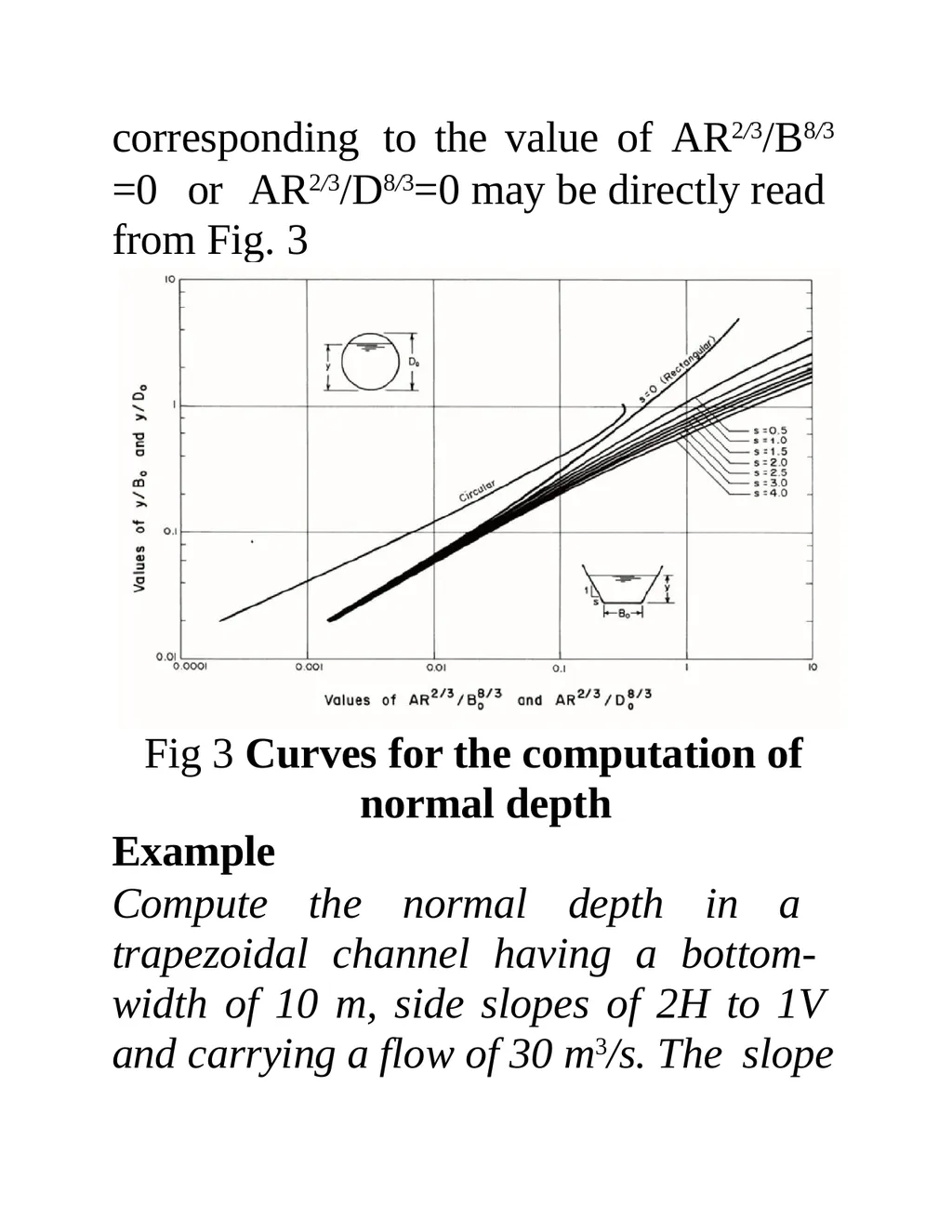
Design Curves
These curves are presented in Fig. 3 for a trapezoidal and for a circular channel section. If we want to determine the normal depth for a specified discharge in a given channel section, then we know Q, n, and So. Therefore, we can compute the right-hand side of Eq. given above. Let us divide this computed value by B8/3
if the channel section is trapezoidal and
by D8/3 if the channel cross section is circular. The resulting value is then equal to AR2/3/B8/3 for a trapezoidal section and equal to AR2/3/D8/3 for a circular cross section. Now, yn/Bo or yn/Do<br>
slide60. corresponding to the value of AR2/3/B8/3
=0 or AR2/3/D8/3=0 may be directly read from Fig. 3 Fig 3 Curves for the computation of normal depth
Example
Compute the normal depth in a trapezoidal channel having a bottom- width of 10 m, side slopes of 2H to 1V and carrying a flow of 30 m3/s. The slope<br>
slide61. of the channel bottom is 0.001 and n =
0.013. Ans yn=1.1
Equivalent Manning Constant
In the previous discussion, we assumed that the flow surface at a channel cross section has the same roughness along the entire wetted perimeter. However, this is not always true. For example, if the channel bottom and sides are made from different materials, then the Manning n different values. To simplify for the bottom and sides may have
the computations, it becomes necessary to determine a value of n, designated by ne, that may be used for the entire section. This value of ne is referred to as the equivalent n for the entire cross section.
Let us consider a channel section that
may be subdivided into N subareas having wetted perimeter Pi and Manning<br>
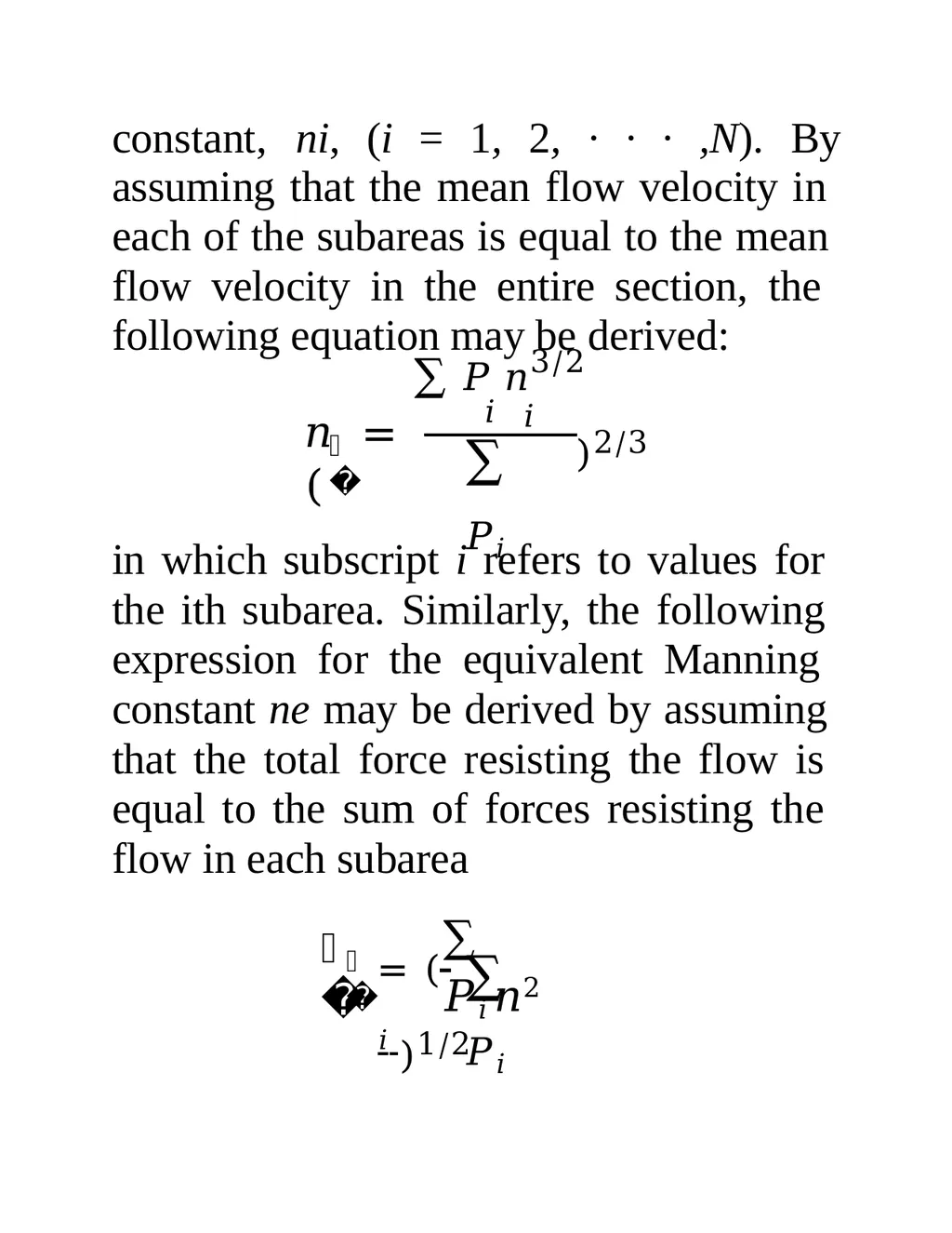
slide62. constant, ni, (i = 1, 2, · · · ,N). By 𝑒 𝑛 = ( 𝑖 𝑖 assuming that the mean flow velocity in each of the subareas is equal to the mean flow velocity in the entire section, the following equation may be derived:
∑ 𝑃 𝑛3/2 ∑ 𝑃𝑖 )2/3 in which subscript i refers to values for the ith subarea. Similarly, the following expression for the equivalent Manning constant ne may be derived by assuming that the total force resisting the flow is equal to the sum of forces resisting the flow in each subarea 𝑛 𝑒 ∑ 𝑃𝑖 𝑛2 ∑ 𝑃𝑖 = ( 𝑖 )1/2<br>
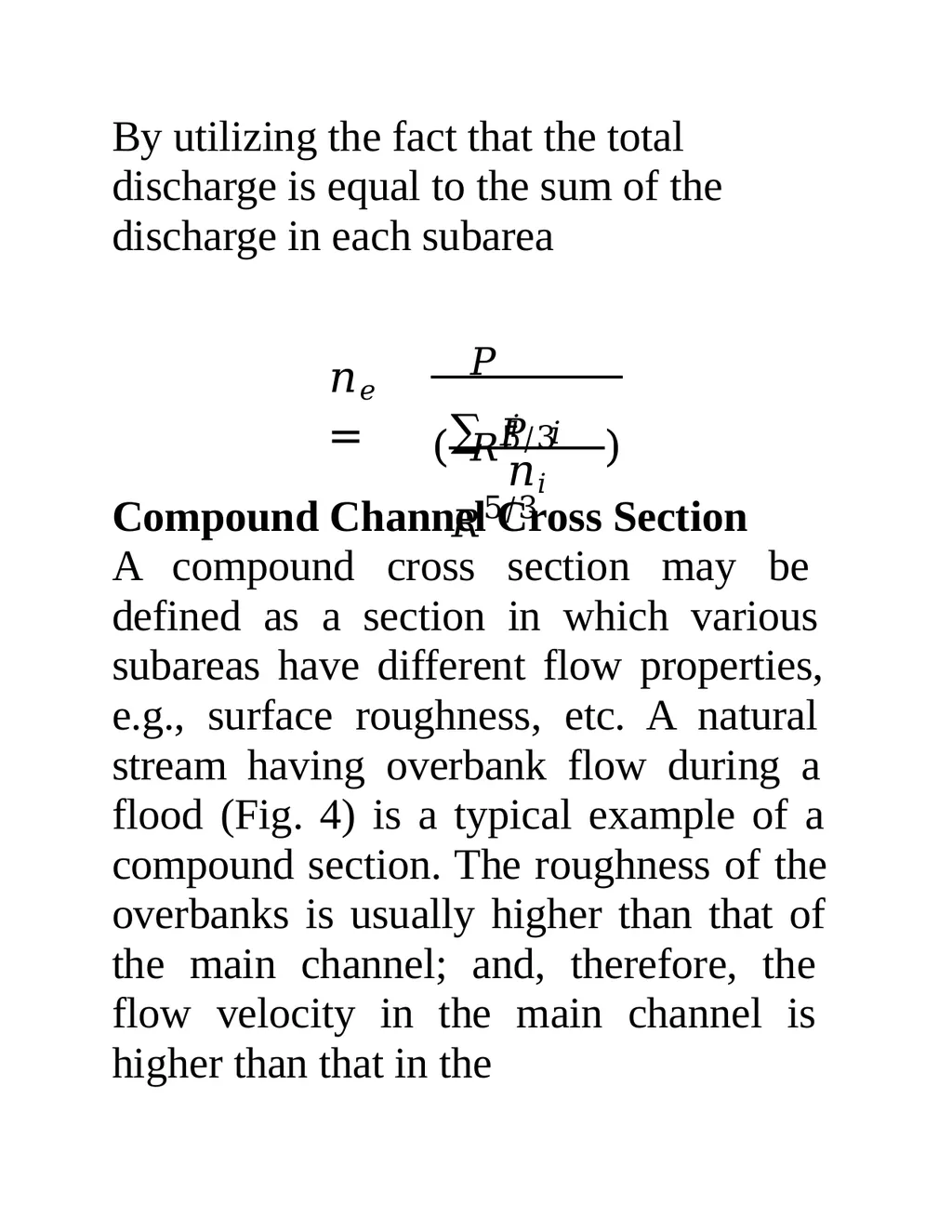
slide63. By utilizing the fact that the total discharge is equal to the sum of the discharge in each subarea 𝑛𝑒 = 𝑃 𝑅5/3 ( 𝑖 𝑖 ∑ 𝑃 𝑅5/3 𝑛𝑖 ) Compound Channel Cross Section
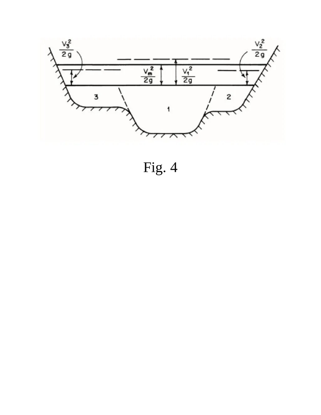
A compound cross section may be defined as a section in which various subareas have different flow properties, e.g., surface roughness, etc. A natural stream having overbank flow during a flood (Fig. 4) is a typical example of a compound section. The roughness of the overbanks is usually higher than that of the main channel; and, therefore, the flow velocity in the main channel is higher than that in the<br>
slide64. The analysis of flow in a compound section becomes complex if the flow in each subarea is considered separately. This requires the use of a two- or three dimensional model or to apply a one- dimensional model separately to each subarea by considering the flow in each sub-area as parallel flow and allowing for the exchange of mass and momentum between the adjacent subareas. In a straight channel, the water surface should be level over the entire cross section, since the pressure along any horizontal line must be constant although the flow velocity may vary from one subarea to the next. Due to different flow velocity, the level of the energy grade line is different in each subarea. Thus, there is no common level for the energy grade line for the entire section. To avoid this<br>
slide65. complexity, we derive in this section expressions for the energy coefficient, α, and for Sf in terms of the conveyance factor, K, of the subareas. With these expressions, the flow in a compound section may be computed without knowing the individual flows in each subarea.
Let us subdivide the compound section
into N subareas. We want to derive an expression for the energy coefficient, α, such that the velocity head for the entire section = αVm 2/ 2g , in which Vm = mean flow velocity in the compound section.<br>
slide66. Fig. 4<br>
slide67. Chapter three GRADUALLY VARIED FLOW
We discussed uniform flow in which the flow depth remains constant with distance. Such flows occur only in long
and prismatic channels (i.e., the channel cross section and bottom slope do not change with distance). In real-life
projects, however, channel cross sections and bottom slopes are not constant with distance in natural channels and these are
varied in constructed channels to suit the<br>
slide68. existing topographical conditions for economic reasons.
In addition, hydraulic structures are provided for flow control. These changes in the channel geometry produce non uniform flows while changing from one uniform-flow condition to another. Such flows are called gradually varied flows if the rate of variation of depth with respect to distance is small, and rapidly varied flows if the rate of variation is large. In other words, the flow depth changes gradually over a long distance in gradually varied flows and in a short distance in rapidly varied flows. Since the analysis of gradually varied flows is usually done for long channels, the friction losses due to boundary shear have to be included. These losses, however, may be neglected in the<br>
slide69. analysis of rapidly varied flows because the distances involved are short. In addition, the pressure distribution in gradually varied flow may be assumed hydrostatic because the streamlines are more or less straight and parallel. However, this is not the case in rapidly acceleration normal to flow varied flows where significant
direction may be produced by sharp curvatures in the streamlines.
Governing Equation
The gradually varied flow equations in a prismatic channel having no lateral inflow or outflow are derived in this section by making the following simplifying assumptions:
1. The slope of the channel bottom is small.<br>
slide70. The channel is prismatic channel and there is no lateral inflow or outflow from the channel.
The pressure distribution is hydrostatic at all channel sections.
4- The head losses in gradually varied flow may be determined by using the equations for head losses in uniform flows.
These assumptions are usually valid for
gradually varied flows. A channel with changing cross section or bottom slope may be divided into piecewise prismatic channels. The slope of the channel bottom may be assumed small if it is less than 5 percent. In such a case, sin θ ~ tan θ ~ θ, in which θ = angle of the channel bottom with horizontal, and the flow depths measured vertically or normal to the bottom are approximately the same.<br>
slide71. The curvature of the streamlines in gradually varied flows is usually small and thus the assumption of hydrostatic pressure distribution is valid. The water- profiles measured during model investigations and surface hydraulic during field observations compare satisfactorily with those computed by using the head-loss equations for steady uniform flow.

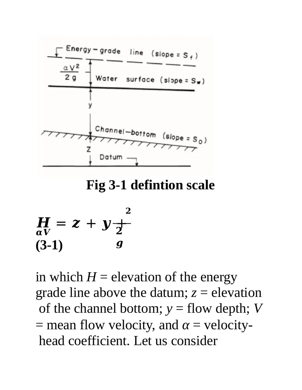
By referring to Fig. 3-1, the total head at a channel section may be written as<br>
slide72. Fig 3-1 defintion scale 𝟐
𝑯 = 𝒛 + 𝒚 + 𝜶𝑽 𝟐𝒈 (3-1)

in which H = elevation of the energy grade line above the datum; z = elevation of the channel bottom; y = flow depth; V
= mean flow velocity, and α = velocity- head coefficient. Let us consider<br>
slide73. distance, x, as positive in the down- 𝑨𝟐 stream flow direction. By differentiating both sides of Eq. 3-1 with respect to x, and expressing V in terms of discharge, Q, we obtain
𝒅𝑯 = 𝒅𝒛 + 𝒅𝒚 + 𝜶𝑸𝟐 𝒅 ( 𝟏 ) 𝒅𝒙 𝒅𝒙 𝒅𝒙 𝟐𝒈 𝒅𝒙
(3-2) Now, by definition 𝒅𝒙 𝒅𝑯 = −𝑺 𝒇 (3-3) 𝒅𝒙 𝒅𝒛 = −𝑺 𝒐 in which Sf = slope of the energy-grade line and So = slope of the channel bottom. There is a negative sign with Sf<br>
slide74. and So since both H and z decrease as x
increases. Now, 𝐝 𝟏 𝐝𝐱 𝐀 ( 𝟐) = ( 𝟐) 𝐝 𝟏 𝐝𝐀 𝐝𝐀 𝐀 𝐝𝐱 = 𝑨𝟐 𝒅 ( 𝟏 ) 𝒅𝑨 𝒅𝒚 𝒅𝑨 𝒅𝒚 𝒅𝒙 ( 3-4) 𝟐𝑩 𝒅𝒚 = −( )
𝑨𝟑 𝒅𝒙 since dA/dy = B,. Note that if the channel is not prismatic, then 𝒅𝑨 = 𝝏𝑨 + 𝝏𝑨 𝒅𝒚
𝒅𝒙 𝝏𝒙 𝝏𝒚 𝒅𝒙 (3-5) and Eqs. 3-4 and 3-5 are modified accordingly, by substituting Eqs. 3-3 and 3-4 into Eq. 3-2, and rearranging the resulting equation, we obtain<br>
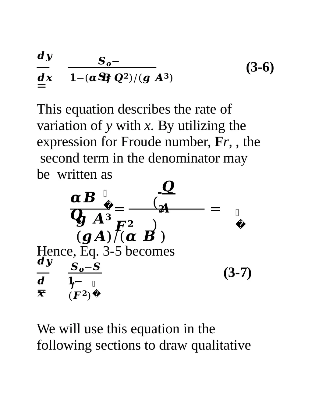
slide75. 𝒅𝒚 = 𝑺𝒐−𝑺𝒇 (3-6) 𝒅𝒙 𝟏−(𝜶 𝑩 𝑸𝟐)/(𝒈 𝑨𝟑)

This equation describes the rate of variation of y with x. By utilizing the expression for Froude number, Fr, , the second term in the denominator may be written as 𝜶𝑩 𝑸 𝟐 (𝑨) 𝑸 𝟐 𝒈 𝑨𝟑 (𝒈𝑨)/(𝜶 𝑩 ) 𝒓 = = 𝑭𝟐 Hence, Eq. 3-5 becomes 𝒅𝒙 𝒅𝒚 = 𝑺𝒐−𝑺𝒇 𝒓 𝟏−(𝑭𝟐) (3-7) We will use this equation in the following sections to draw qualitative<br>
slide76. conclusions about the water-surface profiles.

Classification of Water-Surface Profiles
We use the following notation to designate different water surface profiles: A letter refers to the type of the channel bottom slope and a numeral to the
relative position of the profile with
respect to the critical-depth line (CDL) and the normal-depth line (NDL). The critical depth and the normal depth are yc and yn, respectively.
Channel-bottom slopes are classified into the following five categories:
mild, steep, critical, horizontal (zero
slope) and adverse (negative slope). The first letter of these names refers to the type, i.e., M for mild, S for steep, C for<br>
slide77. critical, H for horizontal and A for adverse slope.
The bottom slope of a channel is called as mild slope if the uniform flow is subcritical (i.e., yn > yc); for the specified
discharge and Manning n; it is critical slope if the uniform flow is critical (i.e., yn = yc); and it is steep slope if the uniform flow is supercritical (i.e., yn <
yc). It is apparent that the normal depth is
infinite if the bottom slope is horizontal and it is nonexistent if the bottom slope is negative. To summarize, the channel bottom slope is called

Mild if yn > yc;
Steep if yn < yc; and
Critical if yn = yc.
Now, let us discuss how to designate the relative position of the surface profile.<br>
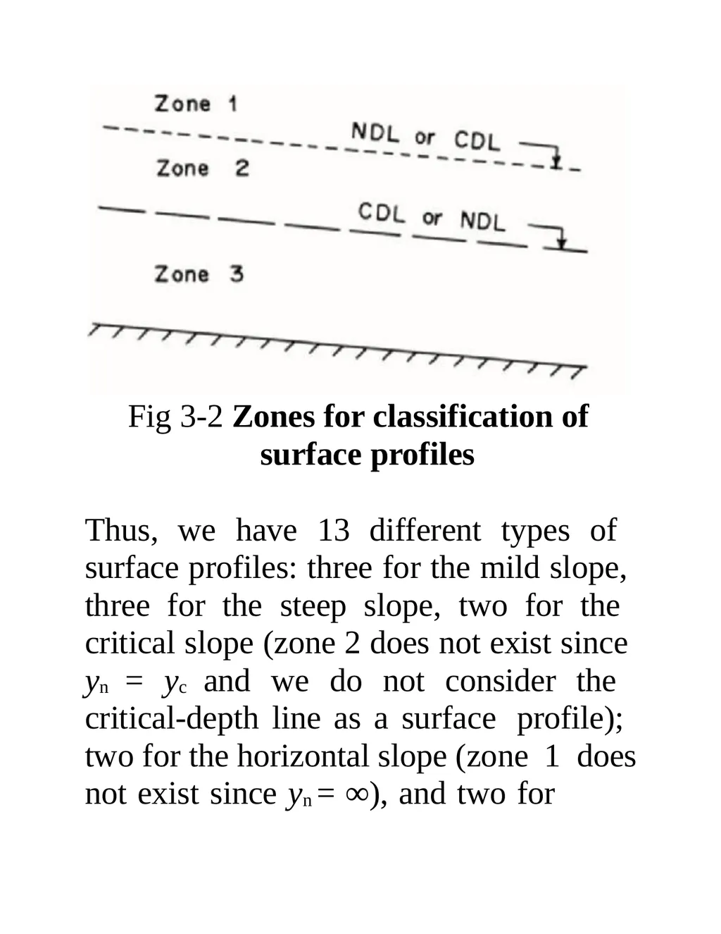
slide78. For the mild and steep slopes, the normal-depth and critical-depth lines divide the space above the channel bottom into three regions, as shown in Fig. 3-2. However, for the adverse, horizontal, and critical bottom slopes, there are only two regions since the normal depth does not exist, is infinite, or is the same as the critical depth, respectively. The region above both lines is designated as Zone 1; that between the upper and lower lines is designated as Zone 2, and the one between the lower line and the channel bottom is designated as Zone 3. Note that the upper line is the normal-depth line if the channel bottom slope is mild, and the upper line is the critical-depth line if the bottom slope is steep.<br>
slide79. Fig 3-2 Zones for classification of surface profiles

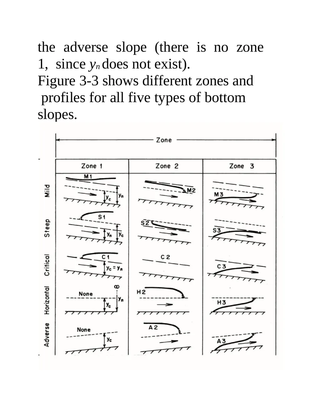
Thus, we have 13 different types of surface profiles: three for the mild slope, three for the steep slope, two for the critical slope (zone 2 does not exist since yn = yc and we do not consider the critical-depth line as a surface profile); two for the horizontal slope (zone 1 does not exist since yn = ∞), and two for<br>
slide80. the adverse slope (there is no zone 1, since yn does not exist).
Figure 3-3 shows different zones and profiles for all five types of bottom slopes.<br>
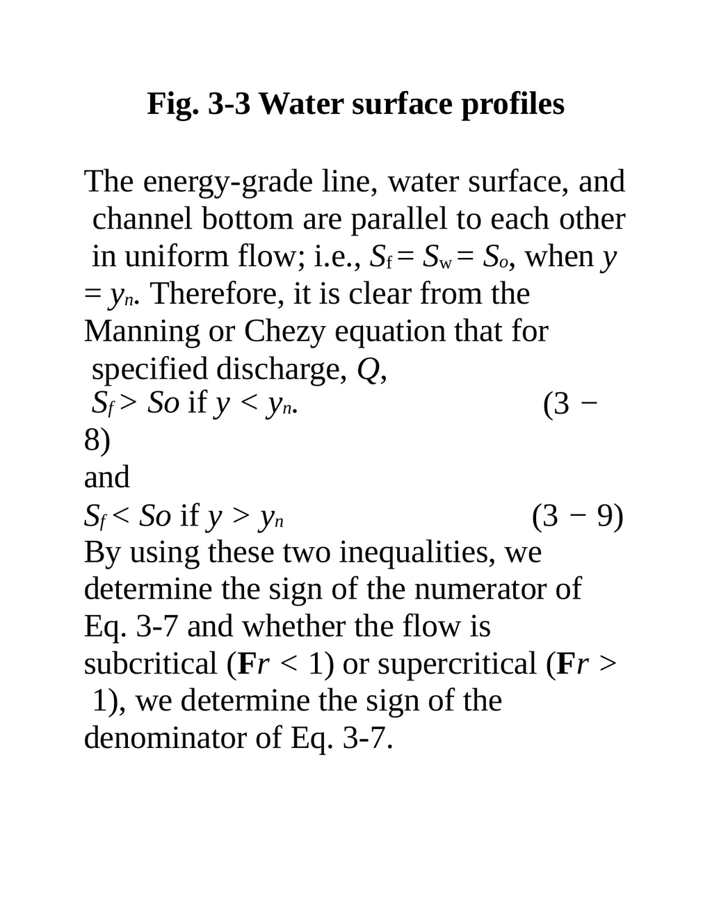
slide81. Fig. 3-3 Water surface profiles

The energy-grade line, water surface, and channel bottom are parallel to each other in uniform flow; i.e., Sf = Sw = So, when y
= yn. Therefore, it is clear from the Manning or Chezy equation that for specified discharge, Q, (3 − Sf > So if y < yn.
8)
and
Sf < So if y > yn (3 − 9) By using these two inequalities, we determine the sign of the numerator of Eq. 3-7 and whether the flow is subcritical (Fr < 1) or supercritical (Fr > 1), we determine the sign of the denominator of Eq. 3-7.<br>
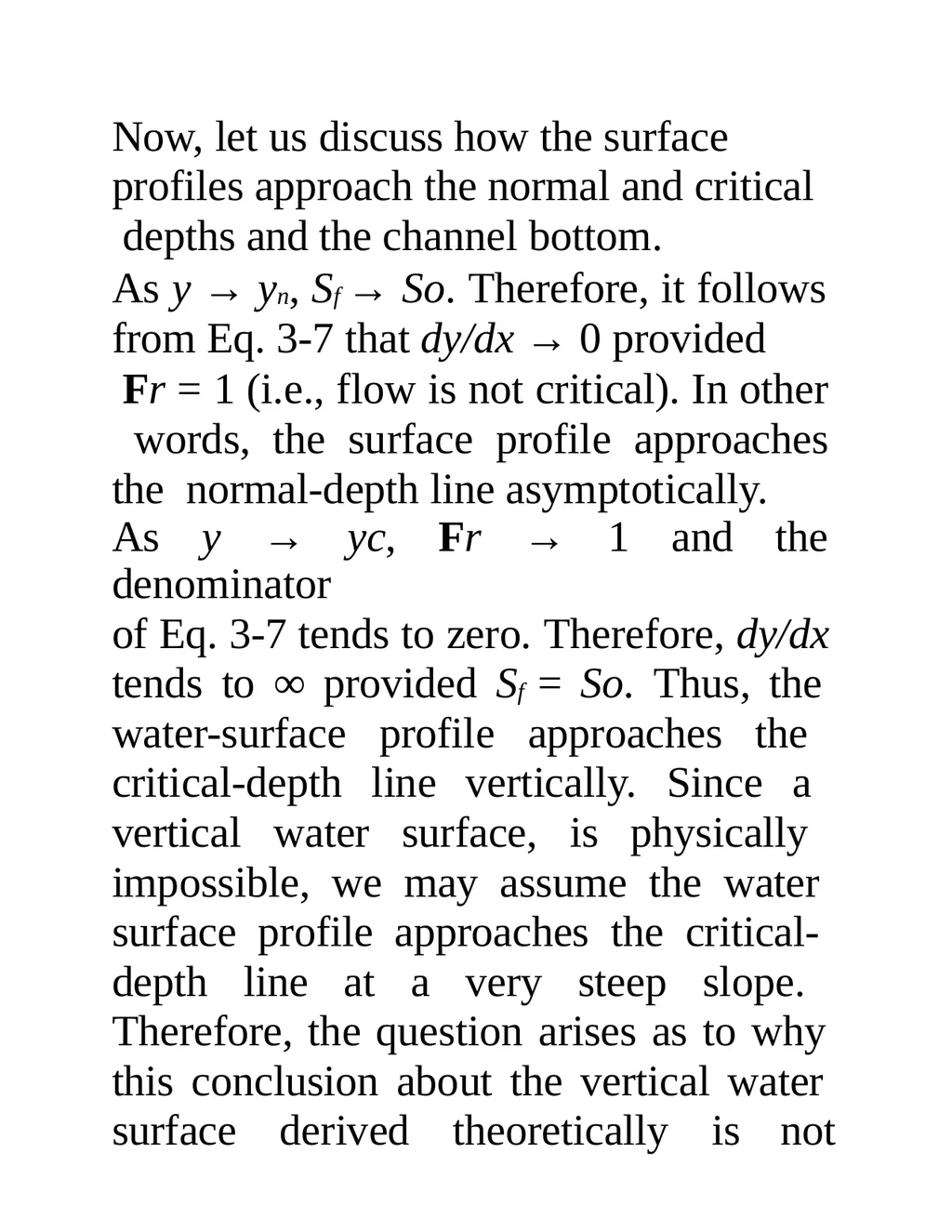
slide82. Now, let us discuss how the surface profiles approach the normal and critical depths and the channel bottom.
As y → yn, Sf → So. Therefore, it follows from Eq. 3-7 that dy/dx → 0 provided
Fr = 1 (i.e., flow is not critical). In other words, the surface profile approaches the normal-depth line asymptotically.
As y → yc, Fr → 1 and the denominator
of Eq. 3-7 tends to zero. Therefore, dy/dx tends to ∞ provided Sf = So. Thus, the water-surface profile approaches the critical-depth line vertically. Since a vertical water surface, is physically impossible, we may assume the water surface profile approaches the critical- depth line at a very steep slope. Therefore, the question arises as to why this conclusion about the vertical water surface derived theoretically is not<br>
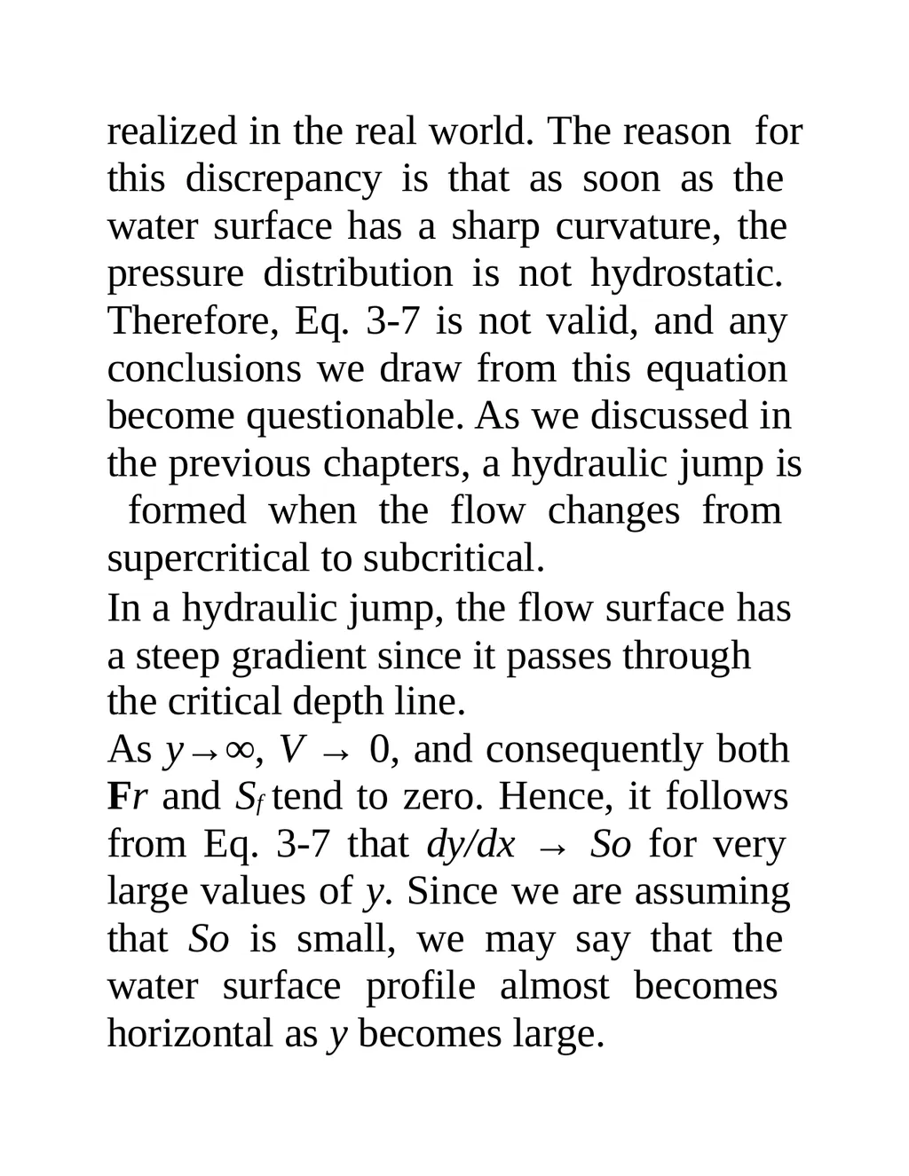
slide83. realized in the real world. The reason for this discrepancy is that as soon as the water surface has a sharp curvature, the pressure distribution is not hydrostatic. Therefore, Eq. 3-7 is not valid, and any conclusions we draw from this equation become questionable. As we discussed in the previous chapters, a hydraulic jump is formed when the flow changes from supercritical to subcritical.
In a hydraulic jump, the flow surface has a steep gradient since it passes through
the critical depth line.
As y→∞, V → 0, and consequently both Fr and Sf tend to zero. Hence, it follows from Eq. 3-7 that dy/dx → So for very large values of y. Since we are assuming that So is small, we may say that the water surface profile almost becomes horizontal as y becomes large.<br>
slide84. Now, let us discuss what happens when the water surface approaches the channel bottom, i.e., y → 0. From the Chezy equation, it follows that<br>