
Outils et methodes A. Tilquin Quelles



Description: Outils et methodes A. Tilquin Quelles statistiques: -Frequentiste -Bayesian Quels outils: -Minimiseur: Minuit -MCMC Freqentist statistic Definition: Probability is interpreted as the frequency of the outcome of a repeatable experiment.
Related Topics
Download Presentation
"Outils et methodes A. Tilquin Quelles" is the property of its rightful owner. Permission is granted to download and print the materials on this website for personal, non-commercial use only, and to display it on your personal computer provided you do not modify the materials and that you retain all copyright notices contained in the materials. By downloading content from our website, you accept the terms of this agreement.
Presentation Transcript
slide1. Outils et methodes
A. Tilquin Quelles statistiques:
-Frequentiste
-Bayesian
Quels outils:
-Minimiseur: Minuit
-MCMC<br>
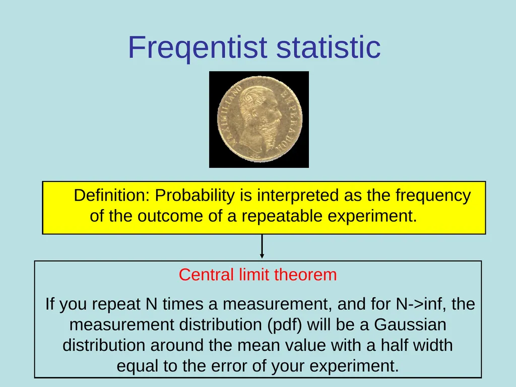
slide2. Freqentist statistic Definition: Probability is interpreted as the frequency of the outcome of a repeatable experiment. Central limit theorem
If you repeat N times a measurement, and for N->inf, the measurement distribution (pdf) will be a Gaussian distribution around the mean value with a half width equal to the error of your experiment.<br>
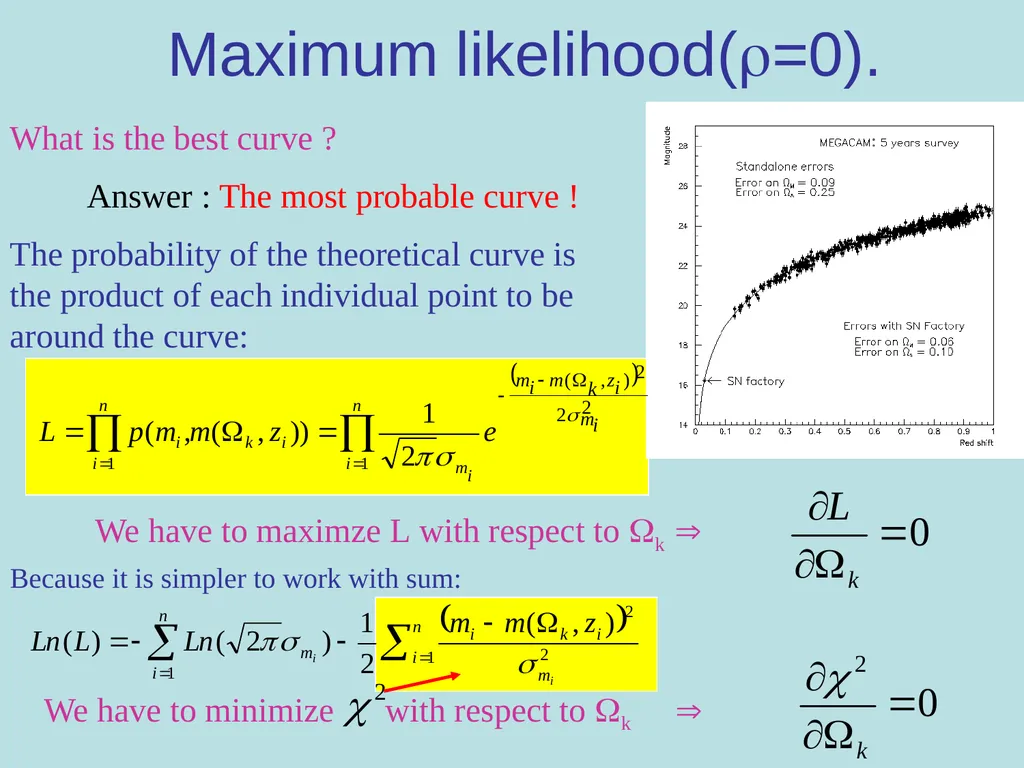
slide3. We have to minimize with respect to k Maximum likelihood(=0). What is the best curve ?
Answer : The most probable curve !
The probability of the theoretical curve is the product of each individual point to be around the curve: We have to maximze L with respect to k Because it is simpler to work with sum: <br>
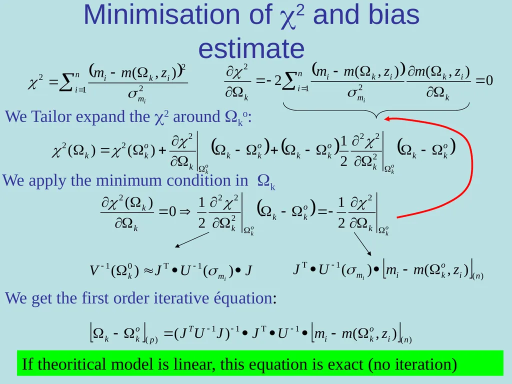
slide4. Minimisation of 2 and bias estimate We Tailor expand the 2 around ko: We apply the minimum condition in k We get the first order iterative équation: If theoritical model is linear, this equation is exact (no iteration)<br>
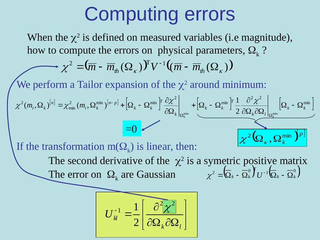
slide5. Computing errors When the 2 is defined on measured variables (i.e magnitude), how to compute the errors on physical parameters, k ? We perform a Tailor expansion of the 2 around minimum: =0 If the transformation m(k) is linear, then:
The second derivative of the 2 is a symetric positive matrix
The error on k are Gaussian<br>
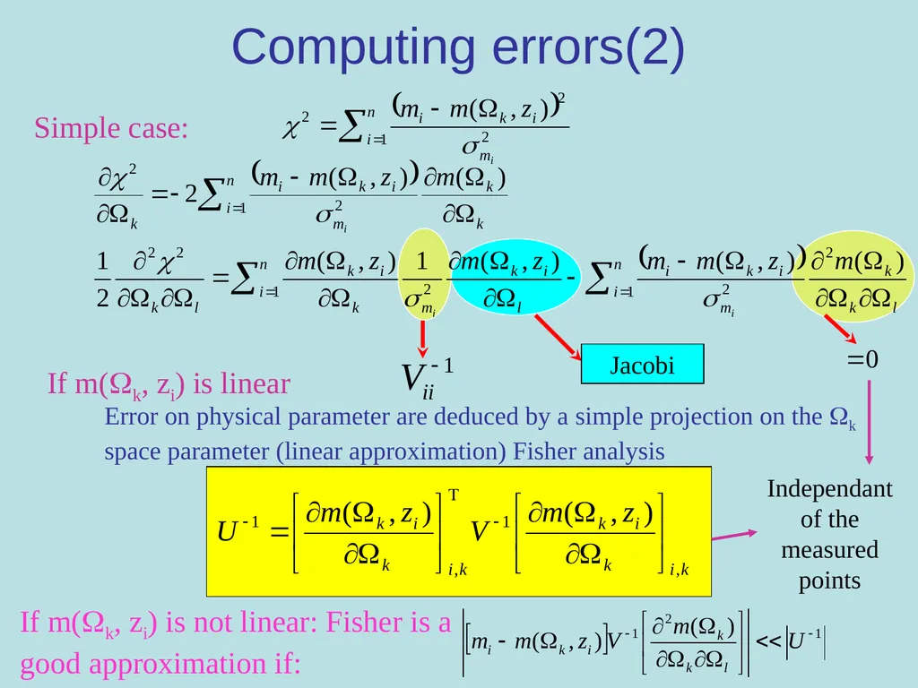
slide6. Computing errors(2) Simple case: If m(k, zi) is linear Jacobi Error on physical parameter are deduced by a simple projection on the k space parameter (linear approximation) Fisher analysis Independant of the measured points If m(k, zi) is not linear: Fisher is a good approximation if:<br>
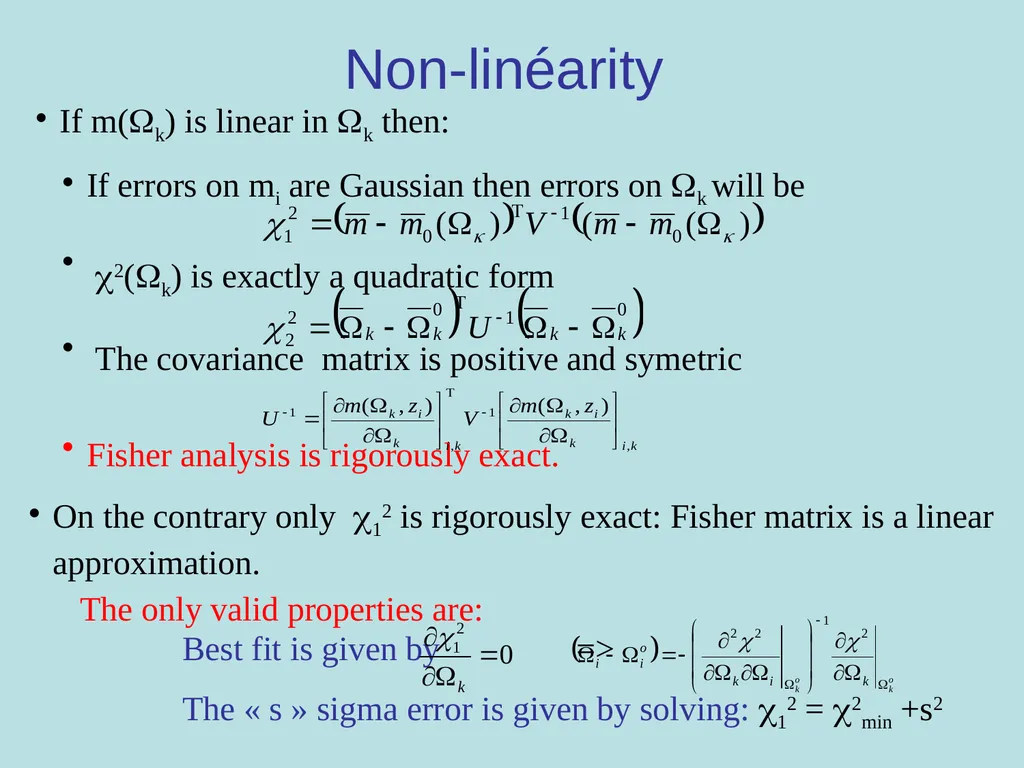
slide7. If m(k) is linear in k then:
If errors on mi are Gaussian then errors on k will be
2(k) is exactly a quadratic form
The covariance matrix is positive and symetric
Fisher analysis is rigorously exact. Non-linéarity On the contrary only 12 is rigorously exact: Fisher matrix is a linear approximation.
The only valid properties are:
Best fit is given by =>
The « s » sigma error is given by solving: 12 = 2min +s2<br>
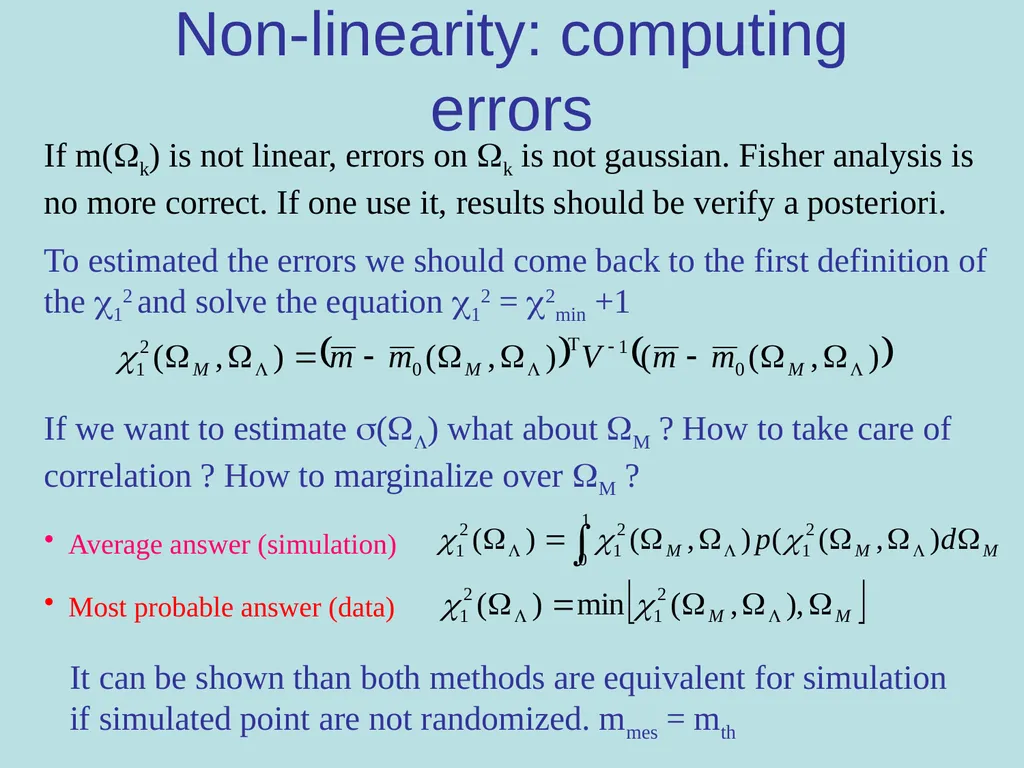
slide8. Non-linearity: computing errors If m(k) is not linear, errors on k is not gaussian. Fisher analysis is no more correct. If one use it, results should be verify a posteriori.
To estimated the errors we should come back to the first definition of the 12 and solve the equation 12 = 2min +1 If we want to estimate () what about M ? How to take care of correlation ? How to marginalize over M ? Average answer (simulation) Most probable answer (data) It can be shown than both methods are equivalent for simulation if simulated point are not randomized. mmes = mth<br>
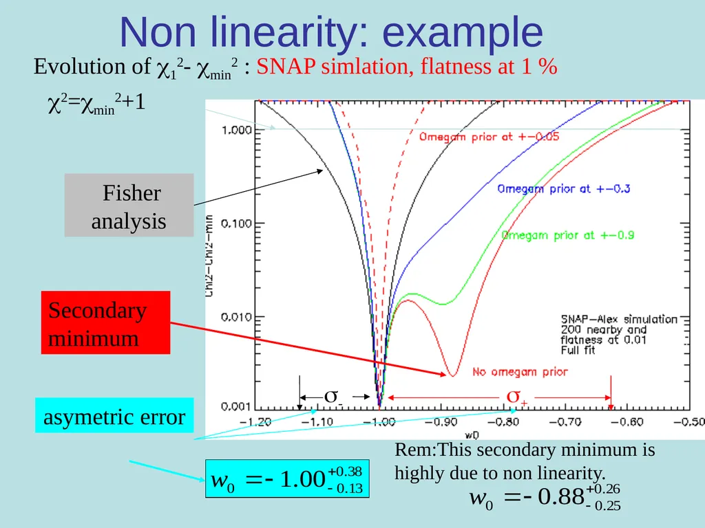
slide9. Non linearity: example Evolution of 12- min2 : SNAP simlation, flatness at 1 % Rem:This secondary minimum is highly due to non linearity.<br>
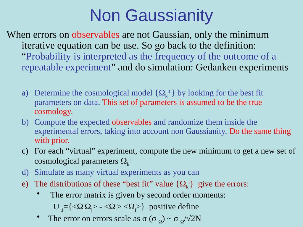
slide10. Non Gaussianity When errors on observables are not Gaussian, only the minimum iterative equation can be use. So go back to the definition: “Probability is interpreted as the frequency of the outcome of a repeatable experiment” and do simulation: Gedanken experiments
Determine the cosmological model {k0 } by looking for the best fit parameters on data. This set of parameters is assumed to be the true cosmology.
Compute the expected observables and randomize them inside the experimental errors, taking into account non Gaussianity. Do the same thing with prior.
For each “virtual” experiment, compute the new minimum to get a new set of cosmological parameters ki
Simulate as many virtual experiments as you can
The distributions of these “best fit” value {ki} give the errors:
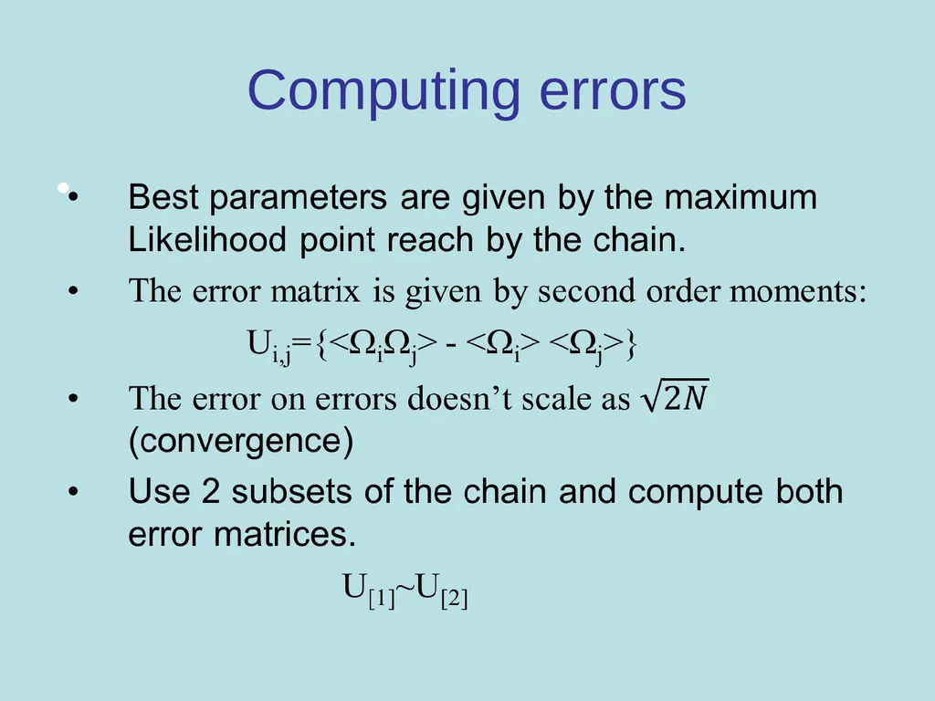
The error matrix is given by second order moments:
Ui,j={<ij> - <i> <j>} positive define
The error on errors scale as σ (σ ) ~ σ /√2N<br>
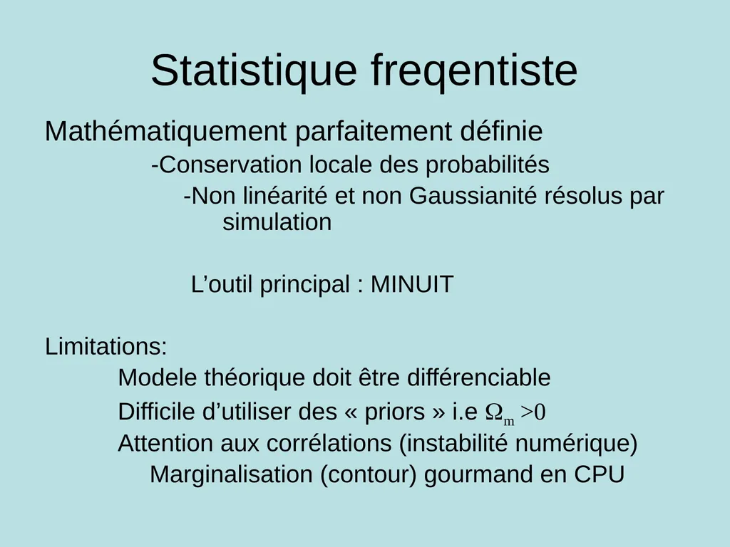
slide11. Statistique freqentiste Mathématiquement parfaitement définie
-Conservation locale des probabilités
-Non linéarité et non Gaussianité résolus par simulation
L’outil principal : MINUIT
Limitations:
Modele théorique doit être différenciable
Difficile d’utiliser des « priors » i.e m >0
Attention aux corrélations (instabilité numérique)
Marginalisation (contour) gourmand en CPU<br>
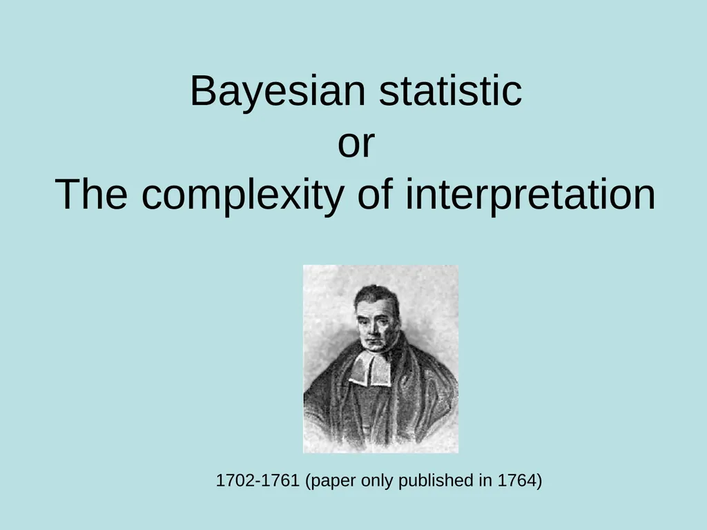
slide12. Bayesian statistic or The complexity of interpretation 1702-1761 (paper only published in 1764)<br>
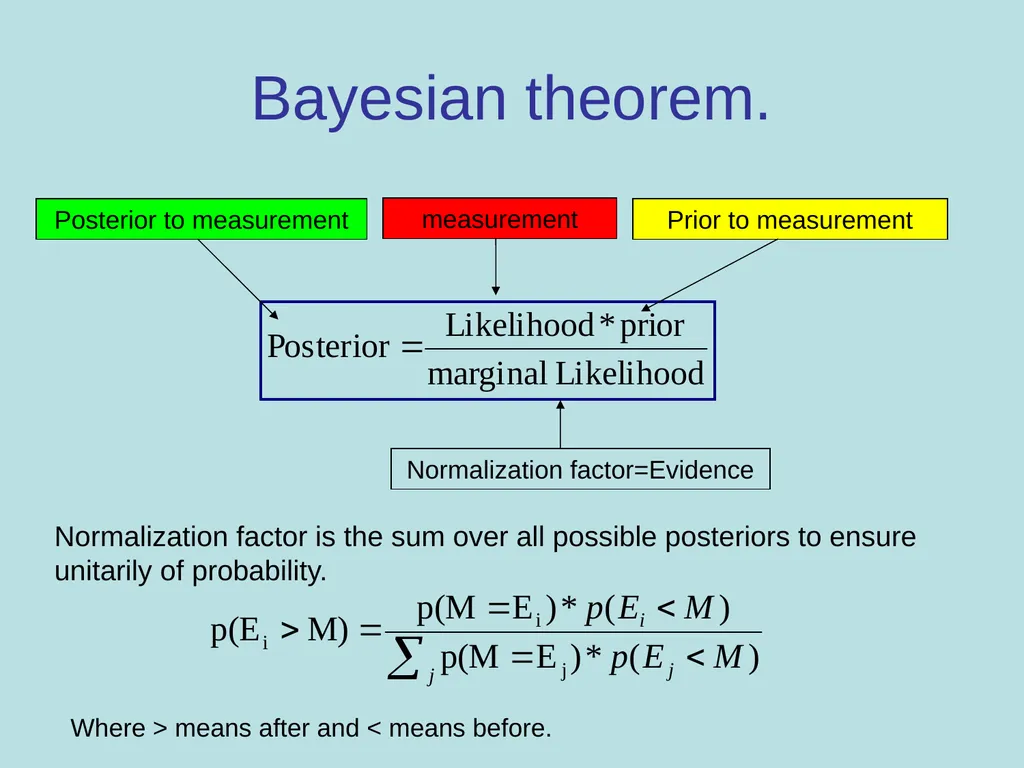
slide13. Bayesian theorem. Prior to measurement measurement Posterior to measurement Normalization factor=Evidence Normalization factor is the sum over all possible posteriors to ensure unitarily of probability. Where > means after and < means before.<br>
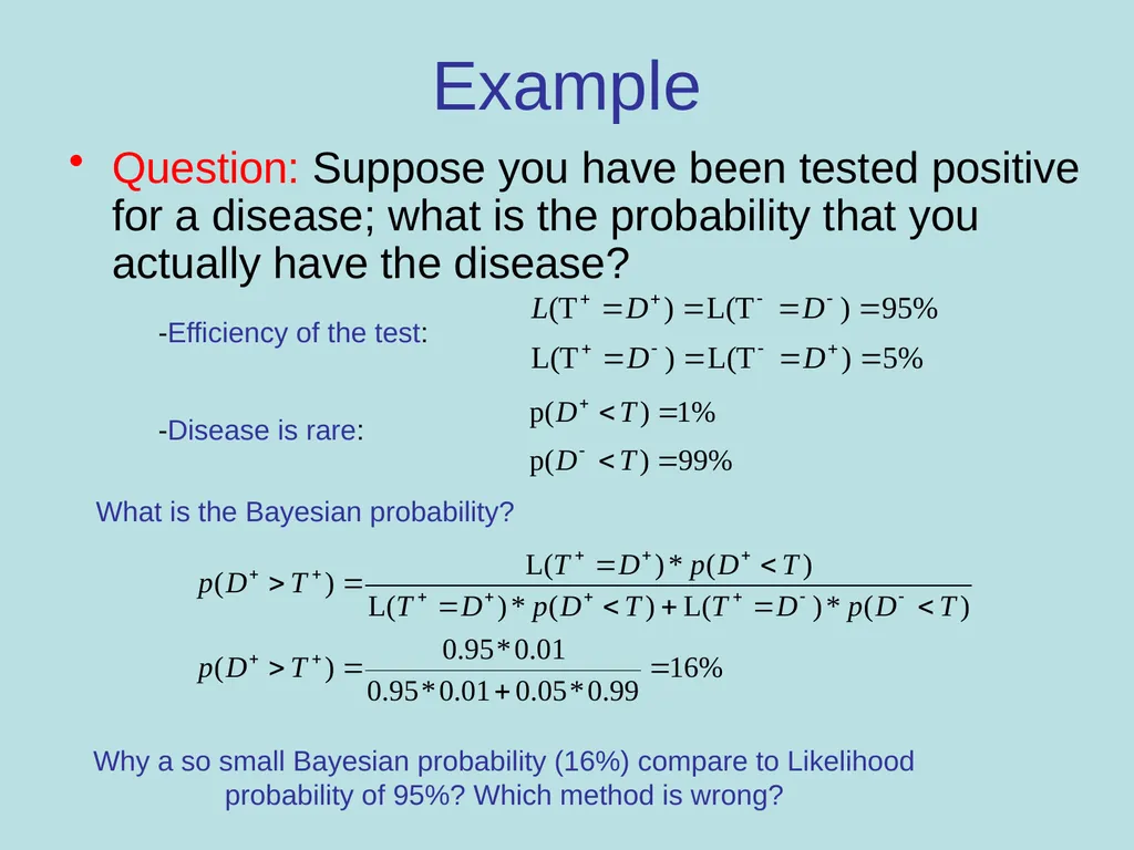
slide14. Example Question: Suppose you have been tested positive for a disease; what is the probability that you actually have the disease? -Efficiency of the test: -Disease is rare: What is the Bayesian probability? Why a so small Bayesian probability (16%) compare to Likelihood probability of 95%? Which method is wrong?<br>
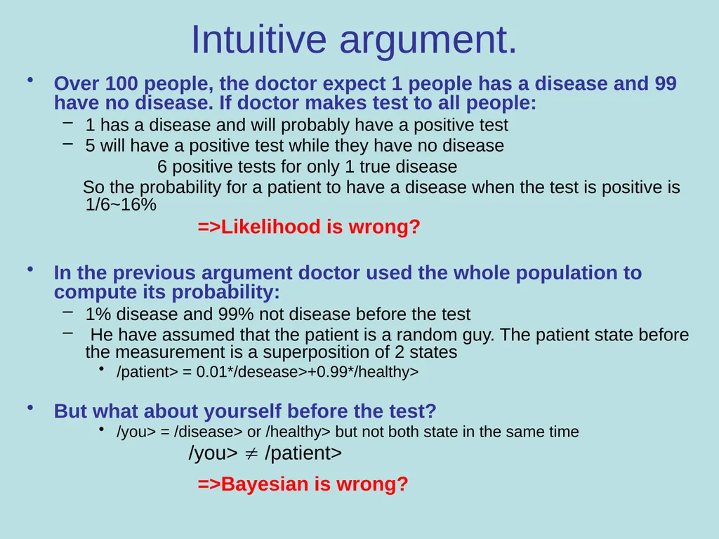
slide15. Intuitive argument. Over 100 people, the doctor expect 1 people has a disease and 99 have no disease. If doctor makes test to all people:
1 has a disease and will probably have a positive test
5 will have a positive test while they have no disease
6 positive tests for only 1 true disease
So the probability for a patient to have a disease when the test is positive is 1/6~16%
=>Likelihood is wrong?
In the previous argument doctor used the whole population to compute its probability:
1% disease and 99% not disease before the test
He have assumed that the patient is a random guy. The patient state before the measurement is a superposition of 2 states
/patient> = 0.01*/desease>+0.99*/healthy>
But what about yourself before the test?
/you> = /disease> or /healthy> but not both state in the same time
/you> /patient>
=>Bayesian is wrong?<br>
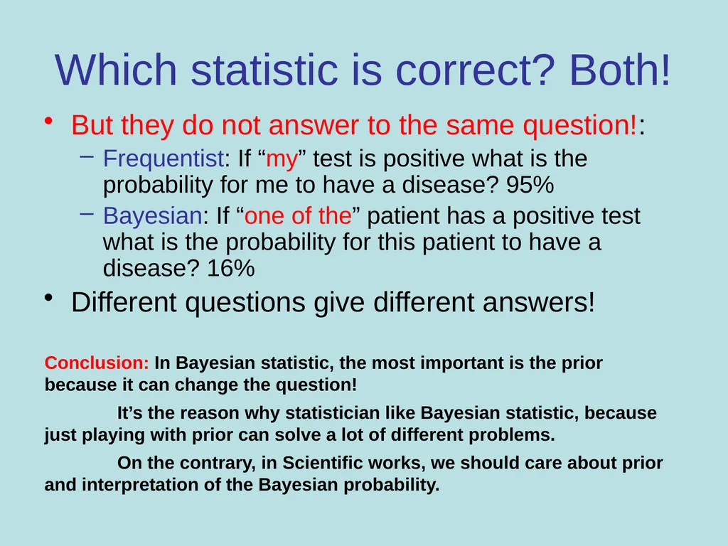
slide16. Which statistic is correct? Both! But they do not answer to the same question!:
Frequentist: If “my” test is positive what is the probability for me to have a disease? 95%
Bayesian: If “one of the” patient has a positive test what is the probability for this patient to have a disease? 16%
Different questions give different answers! Conclusion: In Bayesian statistic, the most important is the prior because it can change the question!
It’s the reason why statistician like Bayesian statistic, because just playing with prior can solve a lot of different problems.
On the contrary, in Scientific works, we should care about prior and interpretation of the Bayesian probability.<br>
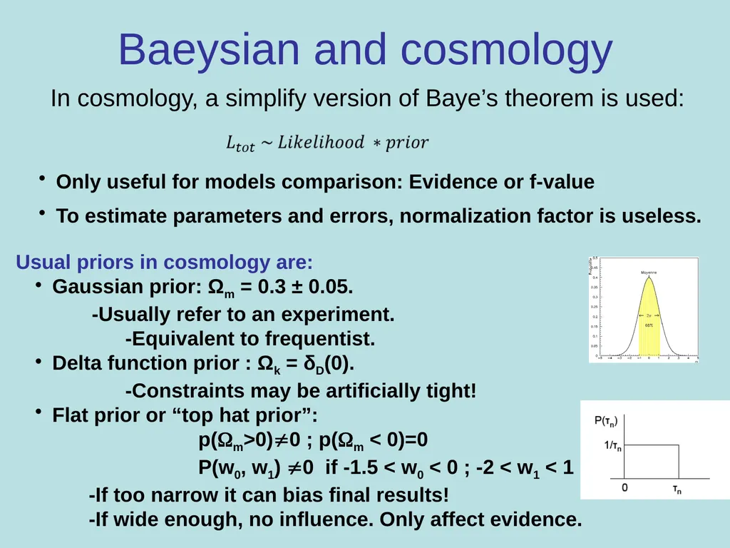
slide17. Baeysian and cosmology In cosmology, a simplify version of Baye’s theorem is used: Usual priors in cosmology are:
Gaussian prior: Ωm = 0.3 ± 0.05.
-Usually refer to an experiment.
-Equivalent to frequentist.
Delta function prior : Ωk = δD(0).
-Constraints may be artificially tight!
Flat prior or “top hat prior”:
p(m>0)0 ; p(m < 0)=0
P(w0, w1) 0 if -1.5 < w0 < 0 ; -2 < w1 < 1
-If too narrow it can bias final results!
-If wide enough, no influence. Only affect evidence. Only useful for models comparison: Evidence or f-value
To estimate parameters and errors, normalization factor is useless.<br>
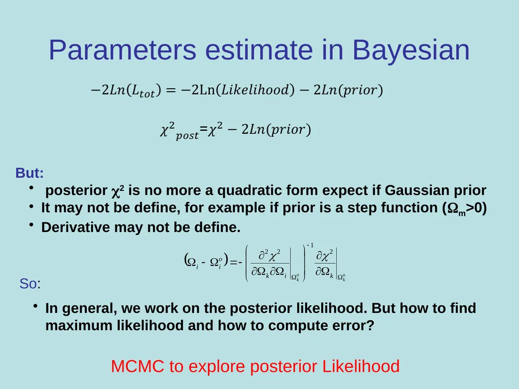
slide18. Parameters estimate in Bayesian But:
posterior 2 is no more a quadratic form expect if Gaussian prior
It may not be define, for example if prior is a step function (m>0)
Derivative may not be define. So:
In general, we work on the posterior likelihood. But how to find maximum likelihood and how to compute error? MCMC to explore posterior Likelihood<br>
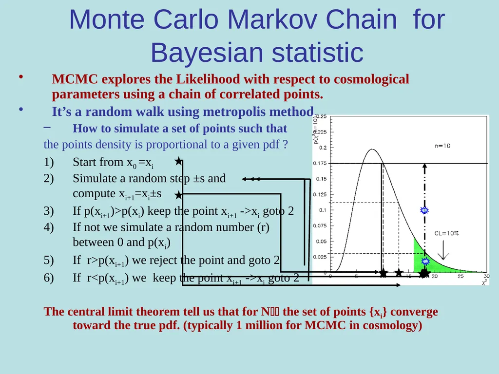
slide19. Monte Carlo Markov Chain for Bayesian statistic MCMC explores the Likelihood with respect to cosmological parameters using a chain of correlated points.
It’s a random walk using metropolis method.
How to simulate a set of points such that
the points density is proportional to a given pdf ?
Start from x0 =xi
Simulate a random step ±s and compute xi+1=xi±s
If p(xi+1)>p(xi) keep the point xi+1 ->xi goto 2
If not we simulate a random number (r) between 0 and p(xi)
If r>p(xi+1) we reject the point and goto 2
If r<p(xi+1) we keep the point xi+1 ->xi goto 2
The central limit theorem tell us that for N the set of points {xi} converge toward the true pdf. (typically 1 million for MCMC in cosmology)<br>
slide20. Computing errors<br>
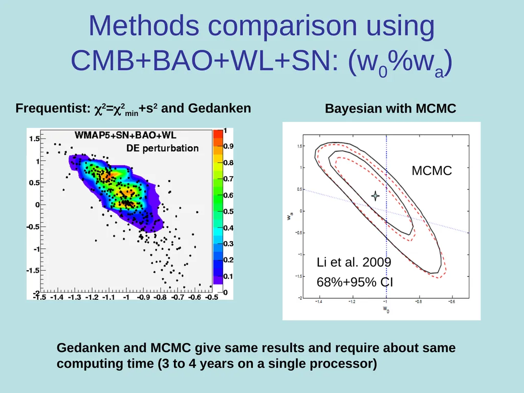
slide21. Methods comparison using CMB+BAO+WL+SN: (w0%wa) Li et al. 2009
68%+95% CI MCMC Frequentist: 2=2min+s2 and Gedanken Bayesian with MCMC Gedanken and MCMC give same results and require about same computing time (3 to 4 years on a single processor)<br>
slide22. Datagrid (DIRAC)<br>
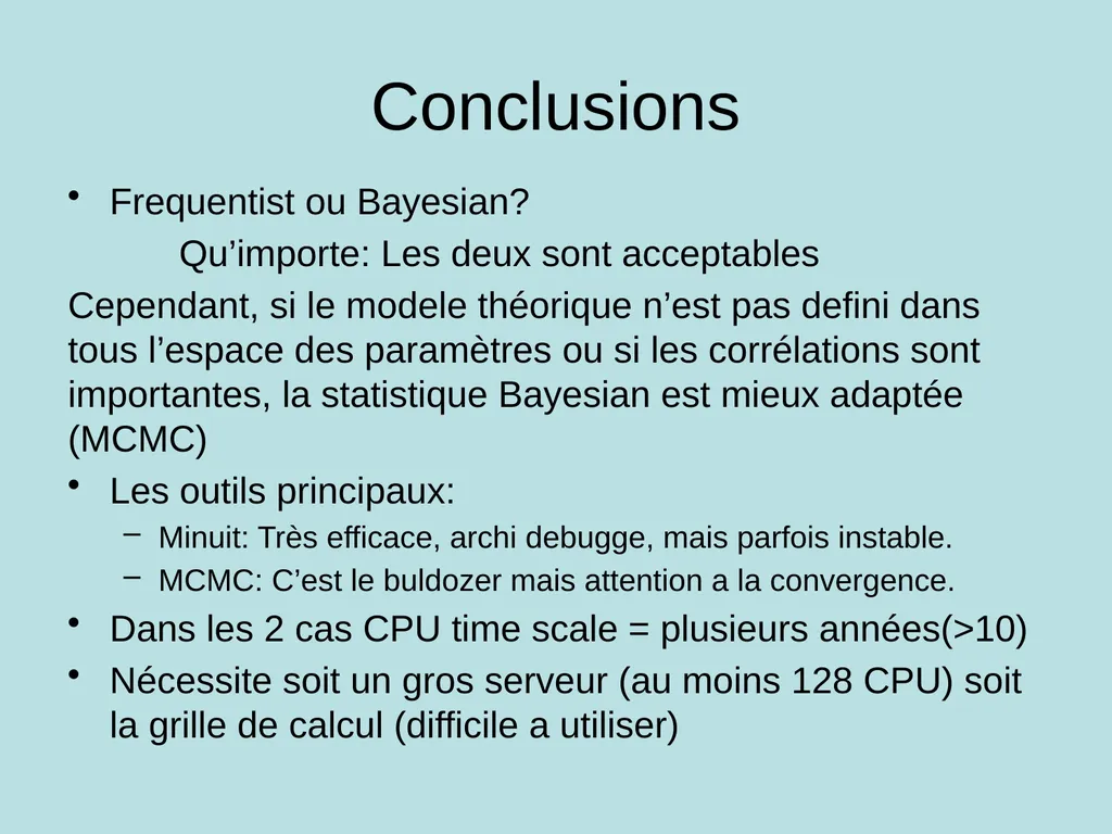
slide23. Conclusions Frequentist ou Bayesian?
Qu’importe: Les deux sont acceptables
Cependant, si le modele théorique n’est pas defini dans tous l’espace des paramètres ou si les corrélations sont importantes, la statistique Bayesian est mieux adaptée (MCMC)
Les outils principaux:
Minuit: Très efficace, archi debugge, mais parfois instable.
MCMC: C’est le buldozer mais attention a la convergence.
Dans les 2 cas CPU time scale = plusieurs années(>10)
Nécessite soit un gros serveur (au moins 128 CPU) soit la grille de calcul (difficile a utiliser)<br>
slide24. Outlook General problem
The frequentist statistic
Likelihood, log-likelihood and 2
Property of the 2
Fisher analysis and limitation
Gedanken experiments
The Bayesian statistic
The Bayes theorem
Example and interpretation.
Prior in cosmology and consequences
MCMC
Summary<br>
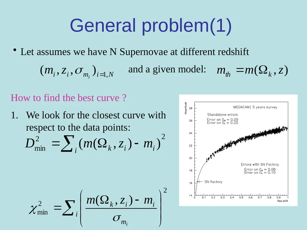
slide25. How to find the best curve ?
We look for the closest curve with respect to the data points:
But the worst measured points should have less weight. General problem(1) Let assumes we have N Supernovae at different redshift
and a given model:<br>
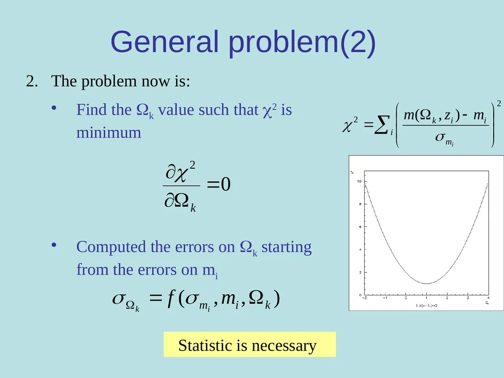
slide26. The problem now is:
Find the k value such that 2 is minimum
Computed the errors on k starting from the errors on mi General problem(2) Statistic is necessary<br>
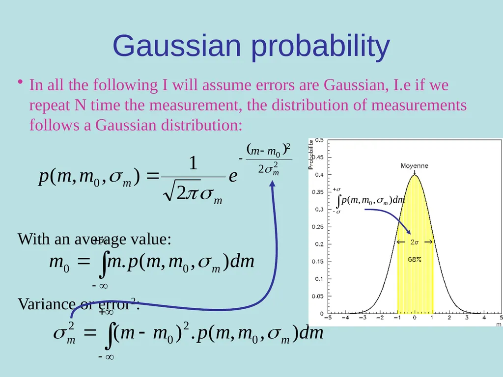
slide27. Gaussian probability In all the following I will assume errors are Gaussian, I.e if we repeat N time the measurement, the distribution of measurements follows a Gaussian distribution:
With an average value:
Variance or error2:<br>
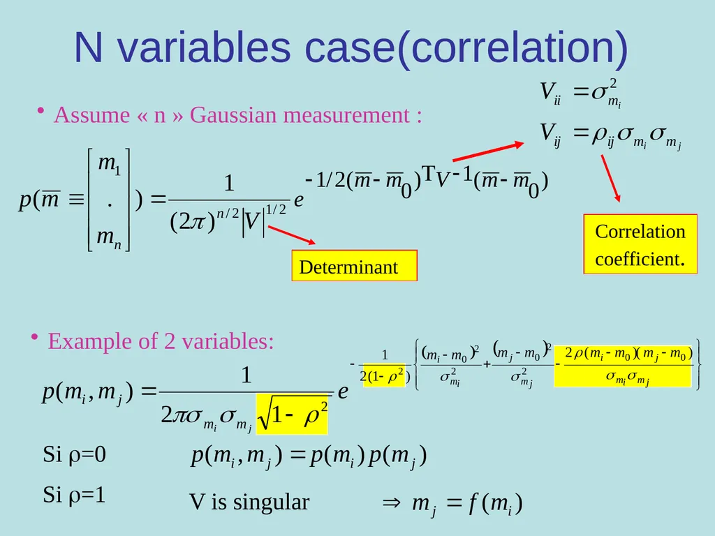
slide28. N variables case(correlation) Assume « n » Gaussian measurement : Correlationcoefficient. Determinant Example of 2 variables: Si =0
Si =1 V is singular<br>
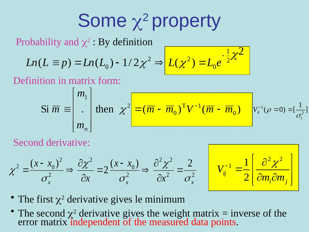
slide29. Some 2 property Definition in matrix form: Second derivative: The first 2 derivative gives le minimum
The second 2 derivative gives the weight matrix = inverse of the error matrix independent of the measured data points. Probability and 2 : By definition<br>
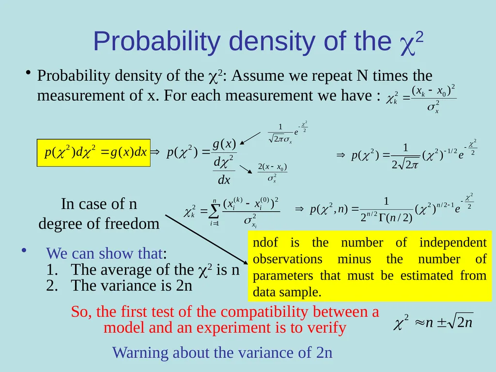
slide30. Probability density of the 2 Probability density of the 2: Assume we repeat N times the measurement of x. For each measurement we have : In case of n degree of freedom We can show that:
The average of the 2 is n
The variance is 2n So, the first test of the compatibility between a model and an experiment is to verify Warning about the variance of 2n ndof is the number of independent observations minus the number of parameters that must be estimated from data sample.<br>
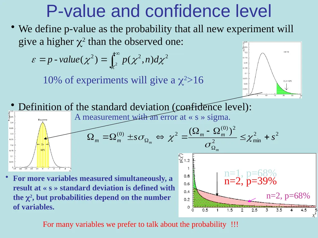
slide31. P-value and confidence level We define p-value as the probability that all new experiment will give a higher 2 than the observed one: 10% of experiments will give a 2>16 Definition of the standard deviation (confidence level):
A measurement with an error at « s » sigma. For more variables measured simultaneously, a result at « s » standard deviation is defined with the 2, but probabilities depend on the number of variables. For many variables we prefer to talk about the probability !!!<br>
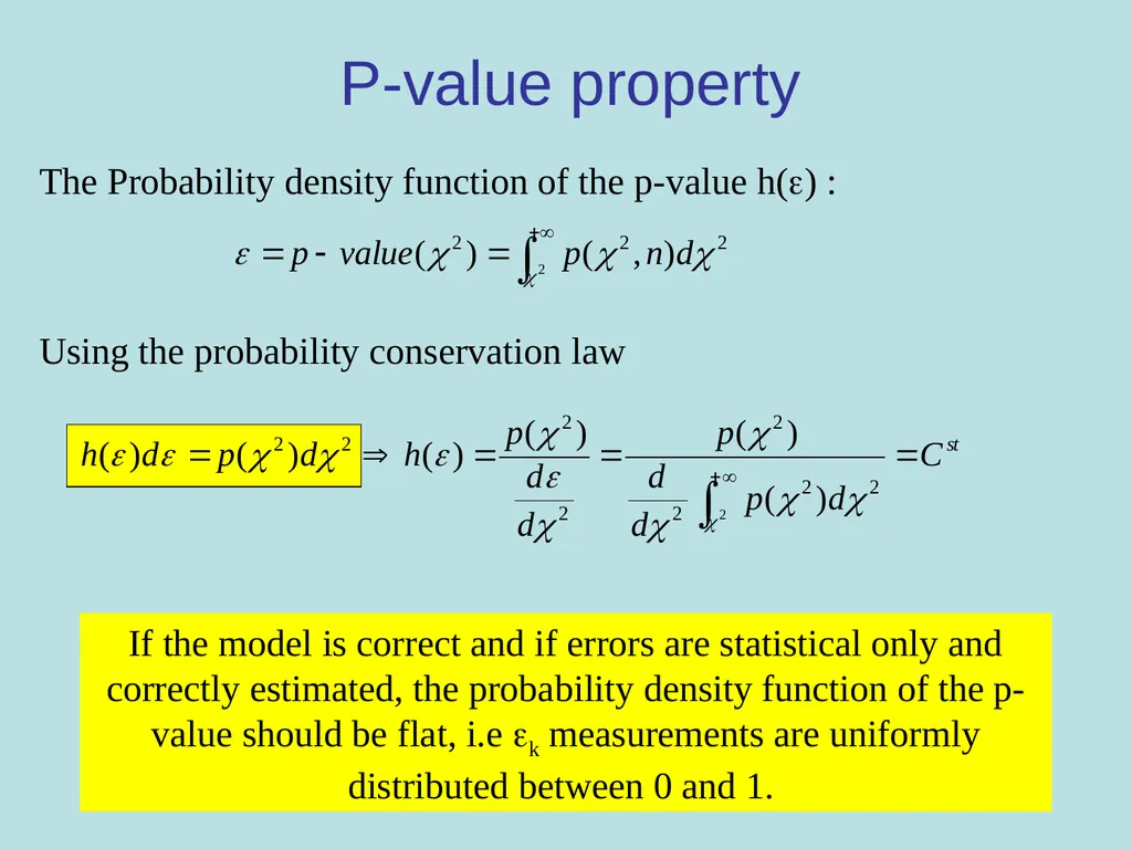
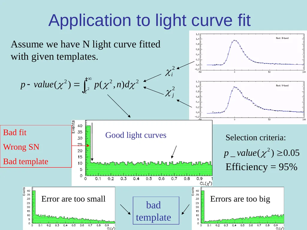
slide32. P-value property The Probability density function of the p-value h() : Using the probability conservation law If the model is correct and if errors are statistical only and correctly estimated, the probability density function of the p-value should be flat, i.e k measurements are uniformly distributed between 0 and 1.<br>
slide33. Application to light curve fit Assume we have N light curve fitted with given templates. Good light curves Bad fit
Wrong SN
Bad template Selection criteria: Error are too small Errors are too big bad template Efficiency = 95%<br>
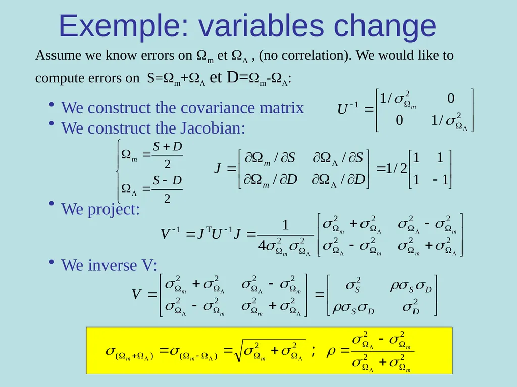
slide34. Assume we know errors on m et , (no correlation). We would like to compute errors on S=m+ et D=m-:
We construct the covariance matrix
We construct the Jacobian:
We project:
We inverse V: Exemple: variables change<br>
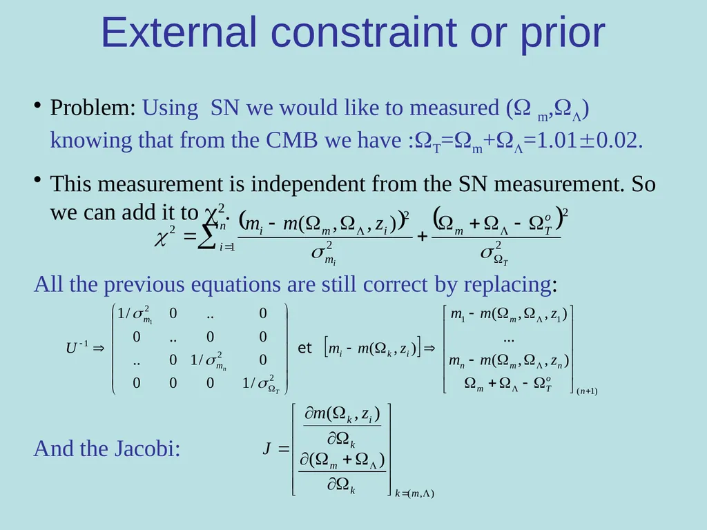
slide35. External constraint or prior Problem: Using SN we would like to measured ( m,) knowing that from the CMB we have :T=m+=1.010.02.
This measurement is independent from the SN measurement. So we can add it to 2. All the previous equations are still correct by replacing: And the Jacobi:<br>
slide36. Online demonstration of MCMC Only if enough time!<br>
slide37. Prior and new discovery In 1999, 2 different groups (SCP and High-z teams) discovered the cosmological constant by using Sn1a at high redshift.
These 2 groups are mainly compose of particle physicists and were using freqentist statistic.
As a consequence they didn’t use prior like m>0… And they made a fundamental discovery!!!<br>
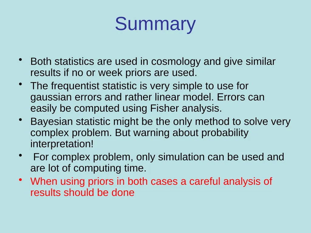
slide38. Summary Both statistics are used in cosmology and give similar results if no or week priors are used.
The frequentist statistic is very simple to use for gaussian errors and rather linear model. Errors can easily be computed using Fisher analysis.
Bayesian statistic might be the only method to solve very complex problem. But warning about probability interpretation!
For complex problem, only simulation can be used and are lot of computing time.
When using priors in both cases a careful analysis of results should be done<br>
slide39. References http://pdg.lbl.gov/2009/reviews/rpp2009-rev-statistics.pdf
http://www.inference.phy.cam.ac.uk/mackay/itila/
http://ipsur.r-forge.r-project.org/
http://www.nu.to.infn.it/Statistics/
http://en.wikipedia.org/wiki/F-distribution
http://www.danielsoper.com/statcalc/calc07.aspx
If you have any question or problem, send me an e-mail: tilquin@cppm.in2p3.fr<br>
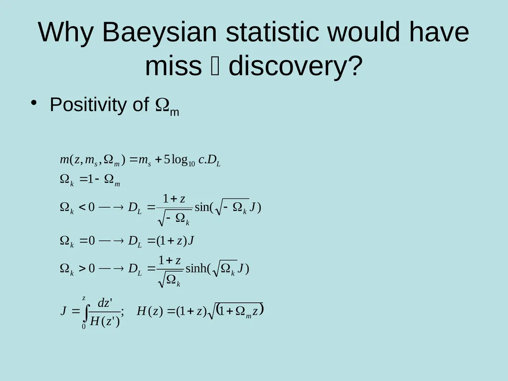
slide40. Why Baeysian statistic would have miss discovery? Positivity of m<br>
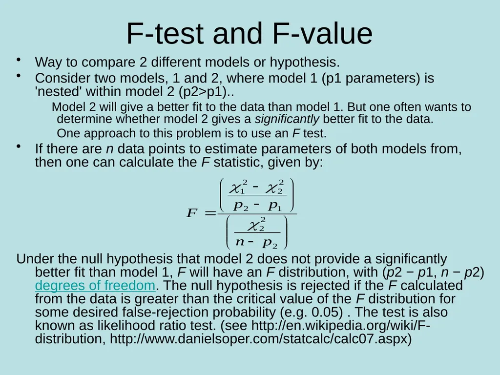
slide41. F-test and F-value Way to compare 2 different models or hypothesis.
Consider two models, 1 and 2, where model 1 (p1 parameters) is 'nested' within model 2 (p2>p1)..
Model 2 will give a better fit to the data than model 1. But one often wants to determine whether model 2 gives a significantly better fit to the data.
One approach to this problem is to use an F test.
If there are n data points to estimate parameters of both models from, then one can calculate the F statistic, given by:
Under the null hypothesis that model 2 does not provide a significantly better fit than model 1, F will have an F distribution, with (p2 − p1, n − p2) degrees of freedom. The null hypothesis is rejected if the F calculated from the data is greater than the critical value of the F distribution for some desired false-rejection probability (e.g. 0.05) . The test is also known as likelihood ratio test. (see http://en.wikipedia.org/wiki/F-distribution, http://www.danielsoper.com/statcalc/calc07.aspx)<br>
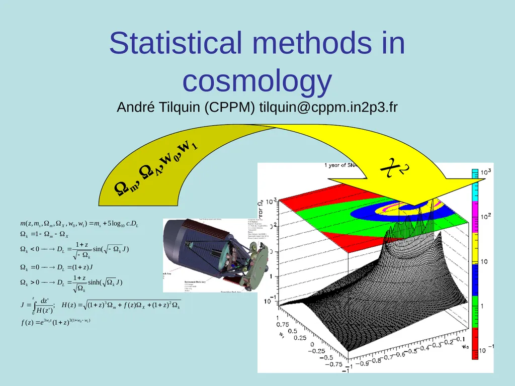
slide42. Statistical methods in cosmology André Tilquin (CPPM) tilquin@cppm.in2p3.fr 2 m, ,w0,w1<br>
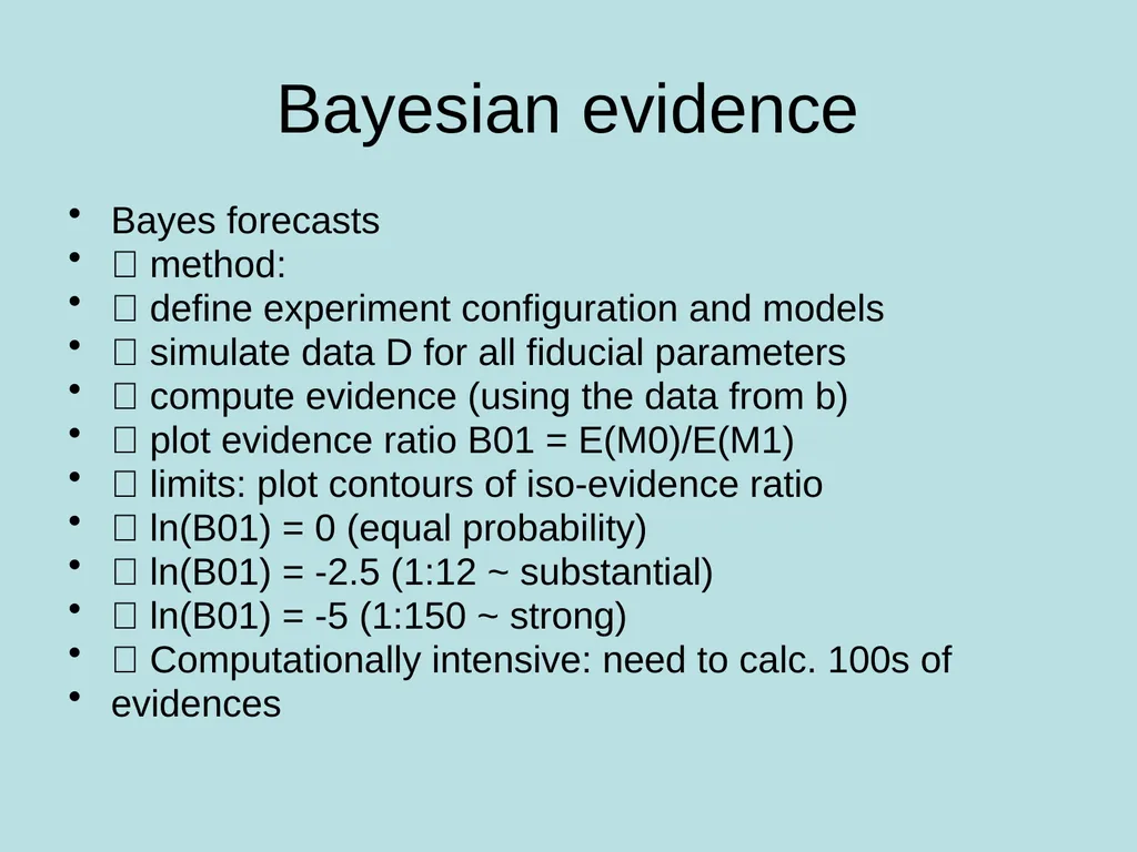
slide43. Bayesian evidence Bayes forecasts
method:
define experiment configuration and models
simulate data D for all fiducial parameters
compute evidence (using the data from b)
plot evidence ratio B01 = E(M0)/E(M1)
limits: plot contours of iso-evidence ratio
ln(B01) = 0 (equal probability)
ln(B01) = -2.5 (1:12 ~ substantial)
ln(B01) = -5 (1:150 ~ strong)
Computationally intensive: need to calc. 100s of
evidences<br>
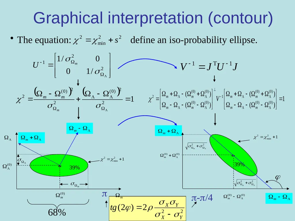
slide44. Graphical interpretation (contour) The equation: define an iso-probability ellipse. -/4 68%<br>
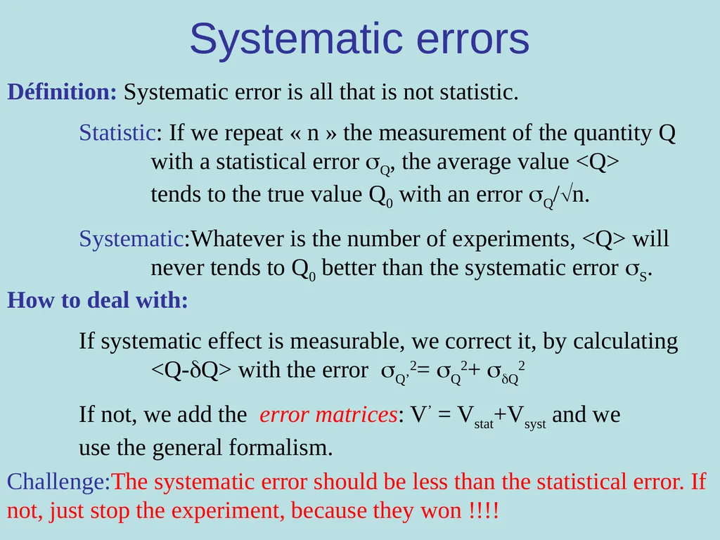
slide45. Systematic errors Définition: Systematic error is all that is not statistic.
Statistic: If we repeat « n » the measurement of the quantity Q with a statistical error Q, the average value <Q> tends to the true value Q0 with an error Q/n.
Systematic:Whatever is the number of experiments, <Q> will never tends to Q0 better than the systematic error S. How to deal with:
If systematic effect is measurable, we correct it, by calculating <Q-Q> with the error Q’2= Q2+ Q2
If not, we add the error matrices: V’ = Vstat+Vsyst and we use the general formalism. Challenge:The systematic error should be less than the statistical error. If not, just stop the experiment, because they won !!!!<br>
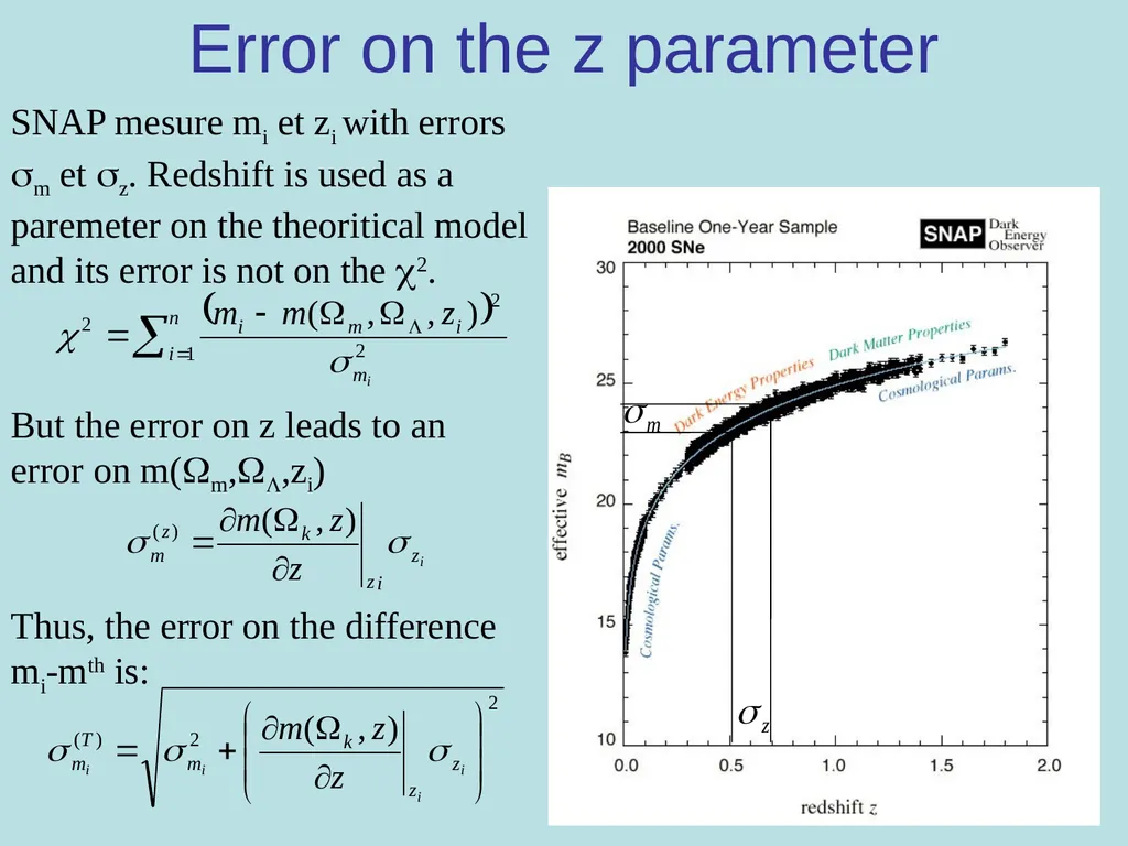
slide46. Error on the z parameter SNAP mesure mi et zi with errors m et z. Redshift is used as a paremeter on the theoritical model and its error is not on the 2. But the error on z leads to an error on m(m,,zi) Thus, the error on the difference mi-mth is:<br>
-Frequentiste
-Bayesian
Quels outils:
-Minimiseur: Minuit
-MCMC<br>
slide2. Freqentist statistic Definition: Probability is interpreted as the frequency of the outcome of a repeatable experiment. Central limit theorem
If you repeat N times a measurement, and for N->inf, the measurement distribution (pdf) will be a Gaussian distribution around the mean value with a half width equal to the error of your experiment.<br>
slide3. We have to minimize with respect to k Maximum likelihood(=0). What is the best curve ?
Answer : The most probable curve !
The probability of the theoretical curve is the product of each individual point to be around the curve: We have to maximze L with respect to k Because it is simpler to work with sum: <br>
slide4. Minimisation of 2 and bias estimate We Tailor expand the 2 around ko: We apply the minimum condition in k We get the first order iterative équation: If theoritical model is linear, this equation is exact (no iteration)<br>
slide5. Computing errors When the 2 is defined on measured variables (i.e magnitude), how to compute the errors on physical parameters, k ? We perform a Tailor expansion of the 2 around minimum: =0 If the transformation m(k) is linear, then:
The second derivative of the 2 is a symetric positive matrix
The error on k are Gaussian<br>
slide6. Computing errors(2) Simple case: If m(k, zi) is linear Jacobi Error on physical parameter are deduced by a simple projection on the k space parameter (linear approximation) Fisher analysis Independant of the measured points If m(k, zi) is not linear: Fisher is a good approximation if:<br>
slide7. If m(k) is linear in k then:
If errors on mi are Gaussian then errors on k will be
2(k) is exactly a quadratic form
The covariance matrix is positive and symetric
Fisher analysis is rigorously exact. Non-linéarity On the contrary only 12 is rigorously exact: Fisher matrix is a linear approximation.
The only valid properties are:
Best fit is given by =>
The « s » sigma error is given by solving: 12 = 2min +s2<br>
slide8. Non-linearity: computing errors If m(k) is not linear, errors on k is not gaussian. Fisher analysis is no more correct. If one use it, results should be verify a posteriori.
To estimated the errors we should come back to the first definition of the 12 and solve the equation 12 = 2min +1 If we want to estimate () what about M ? How to take care of correlation ? How to marginalize over M ? Average answer (simulation) Most probable answer (data) It can be shown than both methods are equivalent for simulation if simulated point are not randomized. mmes = mth<br>
slide9. Non linearity: example Evolution of 12- min2 : SNAP simlation, flatness at 1 % Rem:This secondary minimum is highly due to non linearity.<br>
slide10. Non Gaussianity When errors on observables are not Gaussian, only the minimum iterative equation can be use. So go back to the definition: “Probability is interpreted as the frequency of the outcome of a repeatable experiment” and do simulation: Gedanken experiments
Determine the cosmological model {k0 } by looking for the best fit parameters on data. This set of parameters is assumed to be the true cosmology.
Compute the expected observables and randomize them inside the experimental errors, taking into account non Gaussianity. Do the same thing with prior.
For each “virtual” experiment, compute the new minimum to get a new set of cosmological parameters ki
Simulate as many virtual experiments as you can
The distributions of these “best fit” value {ki} give the errors:
The error matrix is given by second order moments:
Ui,j={<ij> - <i> <j>} positive define
The error on errors scale as σ (σ ) ~ σ /√2N<br>
slide11. Statistique freqentiste Mathématiquement parfaitement définie
-Conservation locale des probabilités
-Non linéarité et non Gaussianité résolus par simulation
L’outil principal : MINUIT
Limitations:
Modele théorique doit être différenciable
Difficile d’utiliser des « priors » i.e m >0
Attention aux corrélations (instabilité numérique)
Marginalisation (contour) gourmand en CPU<br>
slide12. Bayesian statistic or The complexity of interpretation 1702-1761 (paper only published in 1764)<br>
slide13. Bayesian theorem. Prior to measurement measurement Posterior to measurement Normalization factor=Evidence Normalization factor is the sum over all possible posteriors to ensure unitarily of probability. Where > means after and < means before.<br>
slide14. Example Question: Suppose you have been tested positive for a disease; what is the probability that you actually have the disease? -Efficiency of the test: -Disease is rare: What is the Bayesian probability? Why a so small Bayesian probability (16%) compare to Likelihood probability of 95%? Which method is wrong?<br>
slide15. Intuitive argument. Over 100 people, the doctor expect 1 people has a disease and 99 have no disease. If doctor makes test to all people:
1 has a disease and will probably have a positive test
5 will have a positive test while they have no disease
6 positive tests for only 1 true disease
So the probability for a patient to have a disease when the test is positive is 1/6~16%
=>Likelihood is wrong?
In the previous argument doctor used the whole population to compute its probability:
1% disease and 99% not disease before the test
He have assumed that the patient is a random guy. The patient state before the measurement is a superposition of 2 states
/patient> = 0.01*/desease>+0.99*/healthy>
But what about yourself before the test?
/you> = /disease> or /healthy> but not both state in the same time
/you> /patient>
=>Bayesian is wrong?<br>
slide16. Which statistic is correct? Both! But they do not answer to the same question!:
Frequentist: If “my” test is positive what is the probability for me to have a disease? 95%
Bayesian: If “one of the” patient has a positive test what is the probability for this patient to have a disease? 16%
Different questions give different answers! Conclusion: In Bayesian statistic, the most important is the prior because it can change the question!
It’s the reason why statistician like Bayesian statistic, because just playing with prior can solve a lot of different problems.
On the contrary, in Scientific works, we should care about prior and interpretation of the Bayesian probability.<br>
slide17. Baeysian and cosmology In cosmology, a simplify version of Baye’s theorem is used: Usual priors in cosmology are:
Gaussian prior: Ωm = 0.3 ± 0.05.
-Usually refer to an experiment.
-Equivalent to frequentist.
Delta function prior : Ωk = δD(0).
-Constraints may be artificially tight!
Flat prior or “top hat prior”:
p(m>0)0 ; p(m < 0)=0
P(w0, w1) 0 if -1.5 < w0 < 0 ; -2 < w1 < 1
-If too narrow it can bias final results!
-If wide enough, no influence. Only affect evidence. Only useful for models comparison: Evidence or f-value
To estimate parameters and errors, normalization factor is useless.<br>
slide18. Parameters estimate in Bayesian But:
posterior 2 is no more a quadratic form expect if Gaussian prior
It may not be define, for example if prior is a step function (m>0)
Derivative may not be define. So:
In general, we work on the posterior likelihood. But how to find maximum likelihood and how to compute error? MCMC to explore posterior Likelihood<br>
slide19. Monte Carlo Markov Chain for Bayesian statistic MCMC explores the Likelihood with respect to cosmological parameters using a chain of correlated points.
It’s a random walk using metropolis method.
How to simulate a set of points such that
the points density is proportional to a given pdf ?
Start from x0 =xi
Simulate a random step ±s and compute xi+1=xi±s
If p(xi+1)>p(xi) keep the point xi+1 ->xi goto 2
If not we simulate a random number (r) between 0 and p(xi)
If r>p(xi+1) we reject the point and goto 2
If r<p(xi+1) we keep the point xi+1 ->xi goto 2
The central limit theorem tell us that for N the set of points {xi} converge toward the true pdf. (typically 1 million for MCMC in cosmology)<br>
slide20. Computing errors<br>
slide21. Methods comparison using CMB+BAO+WL+SN: (w0%wa) Li et al. 2009
68%+95% CI MCMC Frequentist: 2=2min+s2 and Gedanken Bayesian with MCMC Gedanken and MCMC give same results and require about same computing time (3 to 4 years on a single processor)<br>
slide22. Datagrid (DIRAC)<br>
slide23. Conclusions Frequentist ou Bayesian?
Qu’importe: Les deux sont acceptables
Cependant, si le modele théorique n’est pas defini dans tous l’espace des paramètres ou si les corrélations sont importantes, la statistique Bayesian est mieux adaptée (MCMC)
Les outils principaux:
Minuit: Très efficace, archi debugge, mais parfois instable.
MCMC: C’est le buldozer mais attention a la convergence.
Dans les 2 cas CPU time scale = plusieurs années(>10)
Nécessite soit un gros serveur (au moins 128 CPU) soit la grille de calcul (difficile a utiliser)<br>
slide24. Outlook General problem
The frequentist statistic
Likelihood, log-likelihood and 2
Property of the 2
Fisher analysis and limitation
Gedanken experiments
The Bayesian statistic
The Bayes theorem
Example and interpretation.
Prior in cosmology and consequences
MCMC
Summary<br>
slide25. How to find the best curve ?
We look for the closest curve with respect to the data points:
But the worst measured points should have less weight. General problem(1) Let assumes we have N Supernovae at different redshift
and a given model:<br>
slide26. The problem now is:
Find the k value such that 2 is minimum
Computed the errors on k starting from the errors on mi General problem(2) Statistic is necessary<br>
slide27. Gaussian probability In all the following I will assume errors are Gaussian, I.e if we repeat N time the measurement, the distribution of measurements follows a Gaussian distribution:
With an average value:
Variance or error2:<br>
slide28. N variables case(correlation) Assume « n » Gaussian measurement : Correlationcoefficient. Determinant Example of 2 variables: Si =0
Si =1 V is singular<br>
slide29. Some 2 property Definition in matrix form: Second derivative: The first 2 derivative gives le minimum
The second 2 derivative gives the weight matrix = inverse of the error matrix independent of the measured data points. Probability and 2 : By definition<br>
slide30. Probability density of the 2 Probability density of the 2: Assume we repeat N times the measurement of x. For each measurement we have : In case of n degree of freedom We can show that:
The average of the 2 is n
The variance is 2n So, the first test of the compatibility between a model and an experiment is to verify Warning about the variance of 2n ndof is the number of independent observations minus the number of parameters that must be estimated from data sample.<br>
slide31. P-value and confidence level We define p-value as the probability that all new experiment will give a higher 2 than the observed one: 10% of experiments will give a 2>16 Definition of the standard deviation (confidence level):
A measurement with an error at « s » sigma. For more variables measured simultaneously, a result at « s » standard deviation is defined with the 2, but probabilities depend on the number of variables. For many variables we prefer to talk about the probability !!!<br>
slide32. P-value property The Probability density function of the p-value h() : Using the probability conservation law If the model is correct and if errors are statistical only and correctly estimated, the probability density function of the p-value should be flat, i.e k measurements are uniformly distributed between 0 and 1.<br>
slide33. Application to light curve fit Assume we have N light curve fitted with given templates. Good light curves Bad fit
Wrong SN
Bad template Selection criteria: Error are too small Errors are too big bad template Efficiency = 95%<br>
slide34. Assume we know errors on m et , (no correlation). We would like to compute errors on S=m+ et D=m-:
We construct the covariance matrix
We construct the Jacobian:
We project:
We inverse V: Exemple: variables change<br>
slide35. External constraint or prior Problem: Using SN we would like to measured ( m,) knowing that from the CMB we have :T=m+=1.010.02.
This measurement is independent from the SN measurement. So we can add it to 2. All the previous equations are still correct by replacing: And the Jacobi:<br>
slide36. Online demonstration of MCMC Only if enough time!<br>
slide37. Prior and new discovery In 1999, 2 different groups (SCP and High-z teams) discovered the cosmological constant by using Sn1a at high redshift.
These 2 groups are mainly compose of particle physicists and were using freqentist statistic.
As a consequence they didn’t use prior like m>0… And they made a fundamental discovery!!!<br>
slide38. Summary Both statistics are used in cosmology and give similar results if no or week priors are used.
The frequentist statistic is very simple to use for gaussian errors and rather linear model. Errors can easily be computed using Fisher analysis.
Bayesian statistic might be the only method to solve very complex problem. But warning about probability interpretation!
For complex problem, only simulation can be used and are lot of computing time.
When using priors in both cases a careful analysis of results should be done<br>
slide39. References http://pdg.lbl.gov/2009/reviews/rpp2009-rev-statistics.pdf
http://www.inference.phy.cam.ac.uk/mackay/itila/
http://ipsur.r-forge.r-project.org/
http://www.nu.to.infn.it/Statistics/
http://en.wikipedia.org/wiki/F-distribution
http://www.danielsoper.com/statcalc/calc07.aspx
If you have any question or problem, send me an e-mail: tilquin@cppm.in2p3.fr<br>
slide40. Why Baeysian statistic would have miss discovery? Positivity of m<br>
slide41. F-test and F-value Way to compare 2 different models or hypothesis.
Consider two models, 1 and 2, where model 1 (p1 parameters) is 'nested' within model 2 (p2>p1)..
Model 2 will give a better fit to the data than model 1. But one often wants to determine whether model 2 gives a significantly better fit to the data.
One approach to this problem is to use an F test.
If there are n data points to estimate parameters of both models from, then one can calculate the F statistic, given by:
Under the null hypothesis that model 2 does not provide a significantly better fit than model 1, F will have an F distribution, with (p2 − p1, n − p2) degrees of freedom. The null hypothesis is rejected if the F calculated from the data is greater than the critical value of the F distribution for some desired false-rejection probability (e.g. 0.05) . The test is also known as likelihood ratio test. (see http://en.wikipedia.org/wiki/F-distribution, http://www.danielsoper.com/statcalc/calc07.aspx)<br>
slide42. Statistical methods in cosmology André Tilquin (CPPM) tilquin@cppm.in2p3.fr 2 m, ,w0,w1<br>
slide43. Bayesian evidence Bayes forecasts
method:
define experiment configuration and models
simulate data D for all fiducial parameters
compute evidence (using the data from b)
plot evidence ratio B01 = E(M0)/E(M1)
limits: plot contours of iso-evidence ratio
ln(B01) = 0 (equal probability)
ln(B01) = -2.5 (1:12 ~ substantial)
ln(B01) = -5 (1:150 ~ strong)
Computationally intensive: need to calc. 100s of
evidences<br>
slide44. Graphical interpretation (contour) The equation: define an iso-probability ellipse. -/4 68%<br>
slide45. Systematic errors Définition: Systematic error is all that is not statistic.
Statistic: If we repeat « n » the measurement of the quantity Q with a statistical error Q, the average value <Q> tends to the true value Q0 with an error Q/n.
Systematic:Whatever is the number of experiments, <Q> will never tends to Q0 better than the systematic error S. How to deal with:
If systematic effect is measurable, we correct it, by calculating <Q-Q> with the error Q’2= Q2+ Q2
If not, we add the error matrices: V’ = Vstat+Vsyst and we use the general formalism. Challenge:The systematic error should be less than the statistical error. If not, just stop the experiment, because they won !!!!<br>
slide46. Error on the z parameter SNAP mesure mi et zi with errors m et z. Redshift is used as a paremeter on the theoritical model and its error is not on the 2. But the error on z leads to an error on m(m,,zi) Thus, the error on the difference mi-mth is:<br>