Part 3, Chapter 8 Growth, Inequality and Poverty

slide1. Part 3, Chapter 8Growth, Inequality and Poverty Martin Ravallion Georgetown University course ECON 156: Poverty and Inequality
Lecture notes to accompany Ravallion’s The Economics of Poverty<br>
slide2. 2 We have seen a huge increase in aggregate output<br>
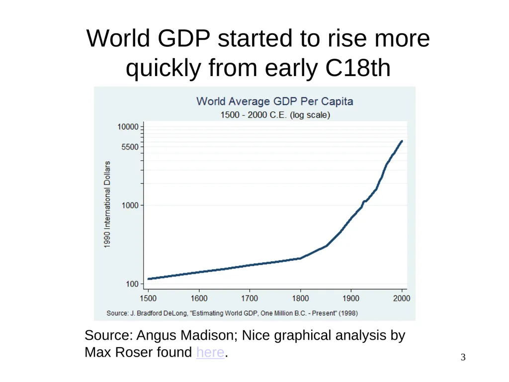
slide3. World GDP started to rise more quickly from early C18th 3 Source: Angus Madison; Nice graphical analysis by
Max Roser found here.<br>
slide4. 4 The questions for this segment: Have poor people participated in this growth? Has inequality risen or fallen?<br>
slide5. Recall that the Classical Economists were pessimistic about “growth with equity” Prominent early Classical economists, such as Malthus and Ricardo, were decidedly pessimistic on the prospects for even reducing poverty, suggesting that they anticipated rising inequality from a growing capitalist economy.
The socialist movement that emerged toward the middle of the 19th century shared the same view, but took it to be a damning criticism of capitalism.
This pessimism about the scope for pro-poor growth continues today. 5<br>
slide6. The debate continued in the C20th In America, during the Second Poverty Enlightenment, J.K. Galbraith and Robert Lampman (prominent advisor to the War on Poverty) had very different views on the scope for poverty reducing growth:
Lampman: post WW2 growth had reduced poverty and this would continue (helped by better social policies)
Galbraith: poverty was now concentrated among sub-groups that would not be able to participate much in future growth. Redistribution is essential. 6<br>
slide7. Conflicting views on growth and poverty “There is plenty of evidence that current patterns of growth and globalization are widening income disparities and hence acting as a brake on poverty reduction.” (Justin Forsyth, Oxfam UK.)
“Globalization policies have contributed to increased poverty, increased inequality between and within nations.” (International Forum for Globalization.)
“…one cannot predict with any confidence that economic growth will translate into reductions in poverty.” (Jeff Shantz)
“It is in the nature of ‘development’ not only to make an overabundance of goods available to consumers but also to produce inequality and exclusion. All the texts on ‘development’ are unanimous in concluding that the gap between North and South (but also between rich and poor in each) is continually widening.” (Gilbert Rist) 7<br>
slide8. Conflicting views cont., “Growth really does help the poor: in fact it raises their incomes by about as much as it raises the incomes of everybody else. Globalization raises incomes, and the poor participate fully.” (The Economist, based on Dollar and Kraay, ‘Growth is Good for the Poor.’)
“Evidence suggests that no one has lost out to globalization in an absolute sense. Growth is sufficient. Period” (Surjit Bhalla, Imagine There’s No Country, Peterson Institute)
“The worst-off benefit far more from trade than the rich.” (The Economist, “Why They’re Wrong.” October 1 2016)
“The gap between the world’s rich and poor will be far narrower in 2050.” Zanny Minton Beddoes (2012) 8<br>
slide9. What are we to make of these differing views?
Are they due to different data or different interpretations of the same data? 9<br>
slide10. 10 Theories of growth and distributional change in developing economies
Evidence from cross-country comparisons Outline<br>
slide11. 11 1. Theories on growth and distribution<br>
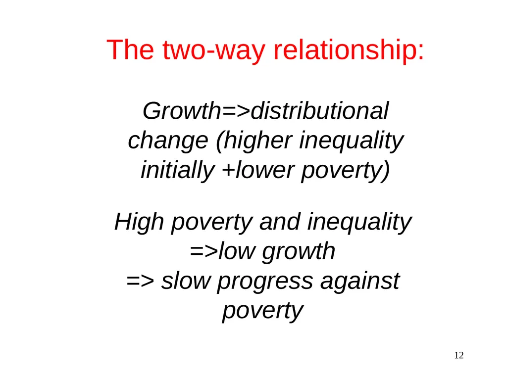
slide12. 12 The two-way relationship:

Growth=>distributional change (higher inequality initially +lower poverty) High poverty and inequality
=>low growth
=> slow progress against poverty<br>
slide13. 13 Growth=>Distribution

Does growth come with rising inequality?
Does growth reduce poverty?<br>
slide14. Economic dualism and structural transformation Food is a necessity for human life, so it is natural that economic activity starts with agriculture.
As the economy grows, the share of output accountable to the (primarily rural) agrarian economy tends to fall.
With overall growth we will tend to see a falling share of income devoted to food: Engel’s Law (Review EOP Box 1.15). 14<br>
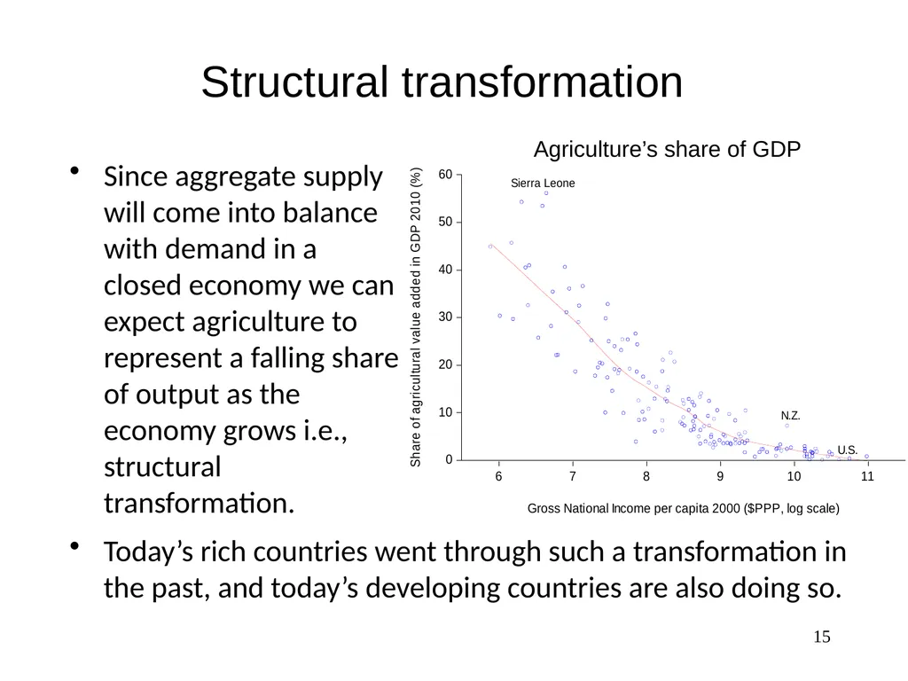
slide15. Structural transformation Since aggregate supply will come into balance with demand in a closed economy we can expect agriculture to represent a falling share of output as the economy grows i.e., structural transformation. 15 Today’s rich countries went through such a transformation in the past, and today’s developing countries are also doing so. Agriculture’s share of GDP<br>
slide16. Caveat: More complex patterns are possible in an open economy In an open economy we may find a degree of country-specialization according to endowments (such as cultivatable land).
This will influence the pattern of sectoral change as the economy grows.
For example, a relatively rich country (such as New Zealand) may still depend heavily on farming because it has an abundance of fertile land, leading it to export its food surplus to buy manufactured goods from a poorer economy without such good land. 16<br>
slide17. Poverty and unemployment The unemployment rate—defined as one’s usual status as looking for work rather than being employed—depends on the level of economic development, notably the extent of formalization in the labor market.
Unemployment as a usual status appears to be more common amongst the non-poor in the developing world.
However, that is not so of underemployment—the time-rate of unemployment (the proportion of time in the workforce spent looking for work).
A common characterization of life in rural areas of a developing country is that most people are doing at least some work, but that they are rarely fully-employed beyond peak seasons in agriculture. 17<br>
slide18. Four models of development in a dualistic market economy A “classical model”: The Lewis model
A “neoclassical model”: Perfect competition
Neoclassical + labor market rigidity: The Harris-Todaro model
Neoclassical + inequality within sectors: The Kuznets curve 18<br>
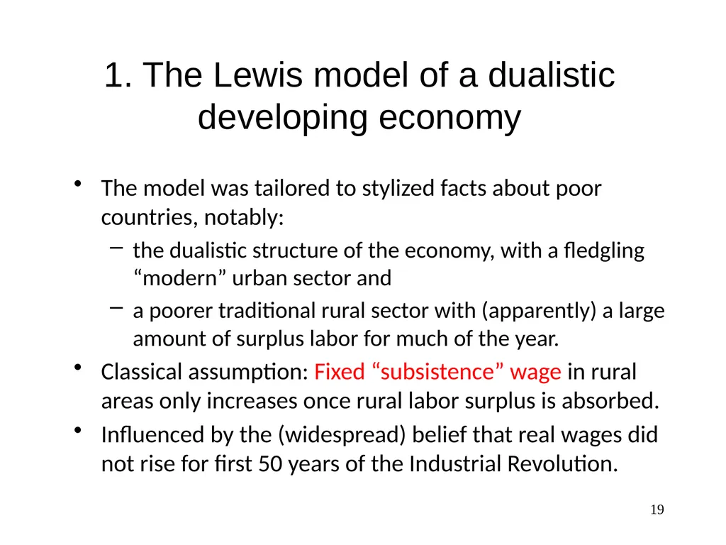
slide19. 1. The Lewis model of a dualistic developing economy The model was tailored to stylized facts about poor countries, notably:
the dualistic structure of the economy, with a fledgling “modern” urban sector and
a poorer traditional rural sector with (apparently) a large amount of surplus labor for much of the year.
Classical assumption: Fixed “subsistence” wage in rural areas only increases once rural labor surplus is absorbed.
Influenced by the (widespread) belief that real wages did not rise for first 50 years of the Industrial Revolution. 19<br>
slide20. Arthur Lewis Born in St. Lucia. Single parent (mother) after age 7.
Completed school at 14 and went to work as a clerk in St Lucia.
Government scholarship to go to University in Britain.
Economics at LSE. Faculty of Manchester then Princeton.
Nobel Prize in Economics 1979, for the Lewis Model.
“The publication of my article on this subject in 1954 was greeted equally with applause and with cries of outrage.” (Arthur Lewis) 20<br>
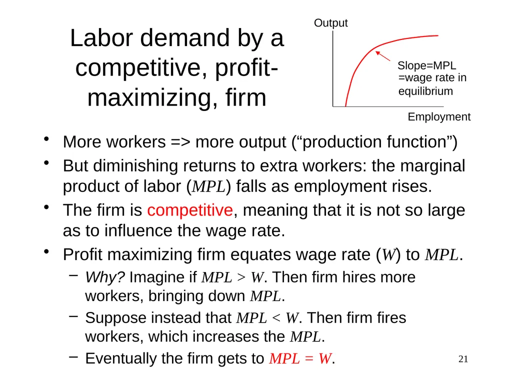
slide21. Labor demand by a competitive, profit-maximizing, firm More workers => more output (“production function”)
But diminishing returns to extra workers: the marginal product of labor (MPL) falls as employment rises.
The firm is competitive, meaning that it is not so large as to influence the wage rate.
Profit maximizing firm equates wage rate (W) to MPL.
Why? Imagine if MPL > W. Then firm hires more workers, bringing down MPL.
Suppose instead that MPL < W. Then firm fires workers, which increases the MPL.
Eventually the firm gets to MPL = W. 21 Employment Output Slope=MPL =wage rate in equilibrium<br>
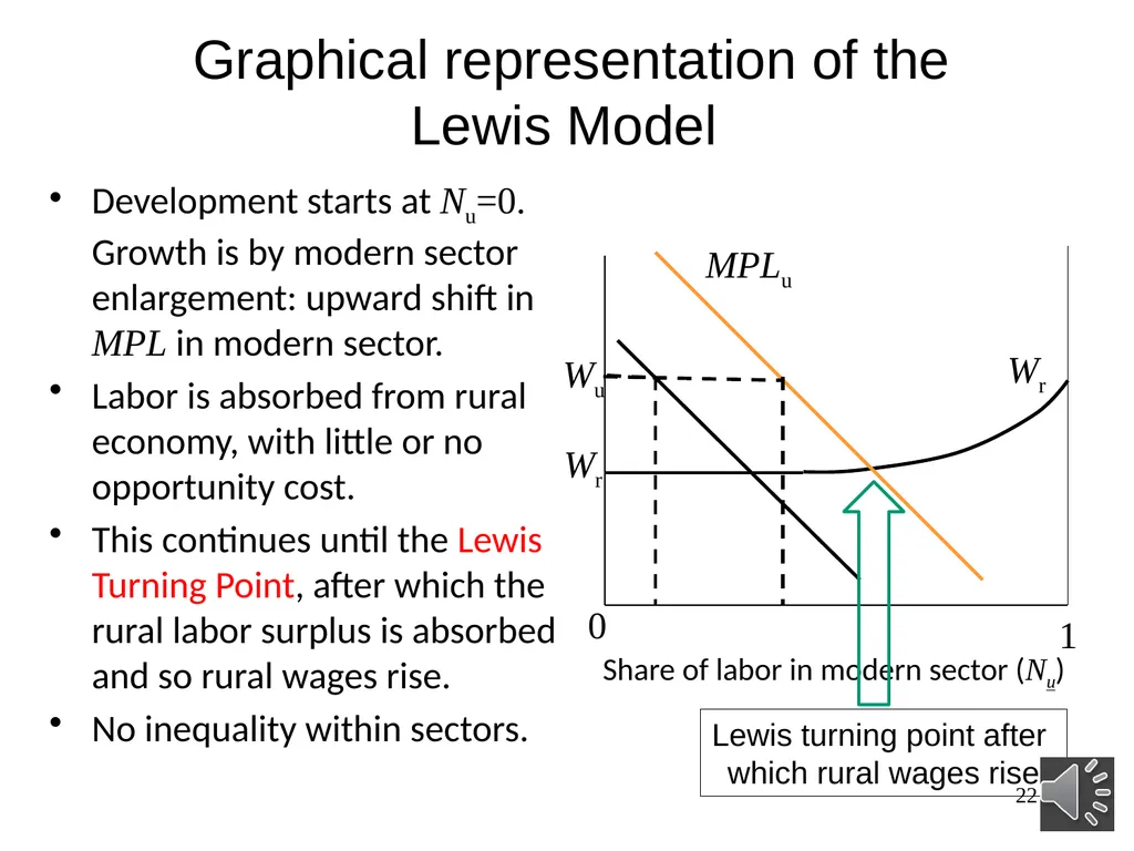
slide22. Graphical representation of the Lewis Model Development starts at Nu=0. Growth is by modern sector enlargement: upward shift in MPL in modern sector.
Labor is absorbed from rural economy, with little or no opportunity cost.
This continues until the Lewis Turning Point, after which the rural labor surplus is absorbed and so rural wages rise.
No inequality within sectors. 22 Wu Wr 0 1 Share of labor in modern sector (Nu) MPLu Lewis turning point after
which rural wages rise Wr<br>
slide23. Reasons for urban-rural wage inequality in the Lewis model Lewis postulated a number of possible reasons for the wage gap (Wu-Wr)
Cost-of-living (but “illusory” in that real wage may be equal)
“Psychological cost” of transferring from rural to urban
“Prestige” of working in modern sector
Capitalist workers organize themselves into a union.
Minimum wage standards in formal sector 23<br>
slide24. Distributional changes during the growth process of the Lewis model Poverty: Ignore inequality within sectors, and assume a poverty line between Wr and Wu.
Poverty incidence falls steadily with modern sector enlargement (and hence economic growth) until poverty is eliminated, sometime after the Lewis Turning Point.
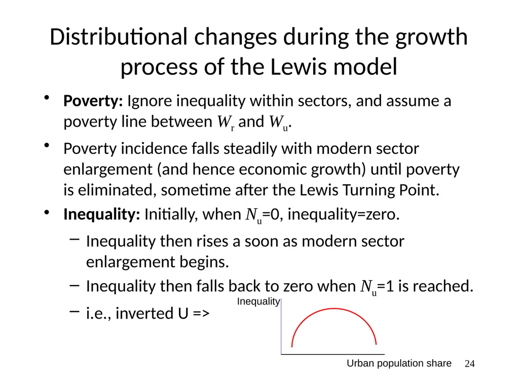
Inequality: Initially, when Nu=0, inequality=zero.
Inequality then rises a soon as modern sector enlargement begins.
Inequality then falls back to zero when Nu=1 is reached.
i.e., inverted U => 24 Inequality Urban population share<br>
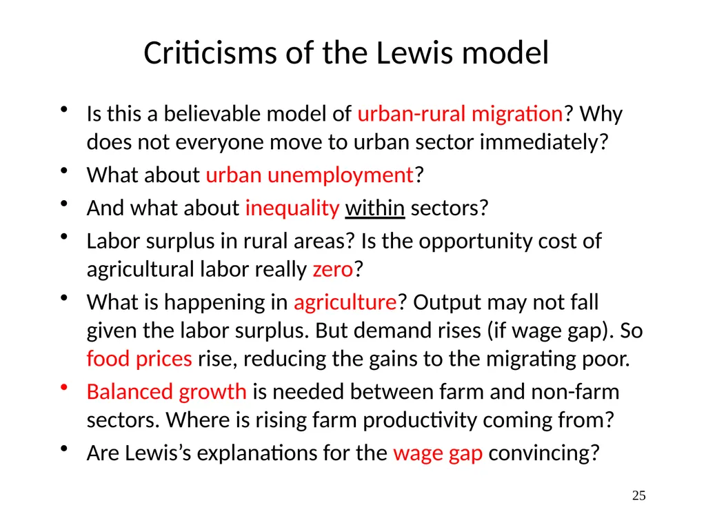
slide25. Criticisms of the Lewis model Is this a believable model of urban-rural migration? Why does not everyone move to urban sector immediately?
What about urban unemployment?
And what about inequality within sectors?
Labor surplus in rural areas? Is the opportunity cost of agricultural labor really zero?
What is happening in agriculture? Output may not fall given the labor surplus. But demand rises (if wage gap). So food prices rise, reducing the gains to the migrating poor.
Balanced growth is needed between farm and non-farm sectors. Where is rising farm productivity coming from?
Are Lewis’s explanations for the wage gap convincing? 25<br>
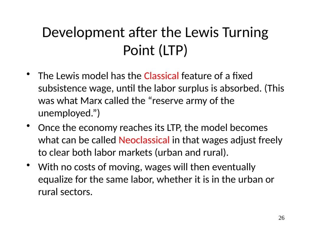
slide26. Development after the Lewis Turning Point (LTP) The Lewis model has the Classical feature of a fixed subsistence wage, until the labor surplus is absorbed. (This was what Marx called the “reserve army of the unemployed.”)
Once the economy reaches its LTP, the model becomes what can be called Neoclassical in that wages adjust freely to clear both labor markets (urban and rural).
With no costs of moving, wages will then eventually equalize for the same labor, whether it is in the urban or rural sectors. 26<br>
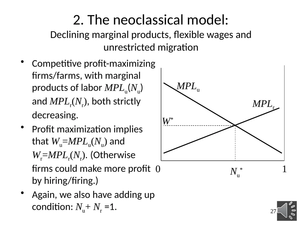
slide27. 2. The neoclassical model:Declining marginal products, flexible wages and unrestricted migration Competitive profit-maximizing firms/farms, with marginal products of labor MPLu(Nu) and MPLr(Nr), both strictly decreasing.
Profit maximization implies that Wu=MPLu(Nu) and Wr=MPLr(Nr). (Otherwise firms could make more profit by hiring/firing.)
Again, we also have adding up condition: Nu+ Nr =1. 27 Nu* MPLu MPLr 0 1 W*<br>
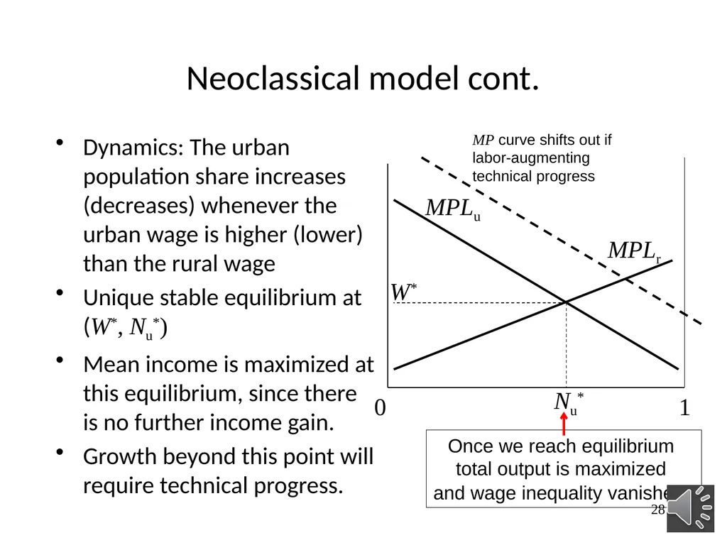
slide28. Neoclassical model cont. Dynamics: The urban population share increases (decreases) whenever the urban wage is higher (lower) than the rural wage
Unique stable equilibrium at (W*, Nu*)
Mean income is maximized at this equilibrium, since there is no further income gain.
Growth beyond this point will require technical progress. 28 Nu* MPLu MPLr 0 1 W* Once we reach equilibrium
total output is maximized
and wage inequality vanishes. MP curve shifts out if
labor-augmenting
technical progress<br>
slide29. Introducing labor-market segmentation and urban unemployment No urban unemployment in the last two models. But this is a common concern, esp., young unemployed in cities.
A famous example of a development policy with unintended consequence:
In 1964 the Kenyan government tried to reduce urban unemployment by providing extra jobs in the cities.
Unexpected outcome: The chance of getting one of these new jobs attracted new workers from rural areas to Nairobi.
And so many rural workers came that the urban unemployment rate actually rose.
This was the motivation of the Harris-Todaro model. 29<br>
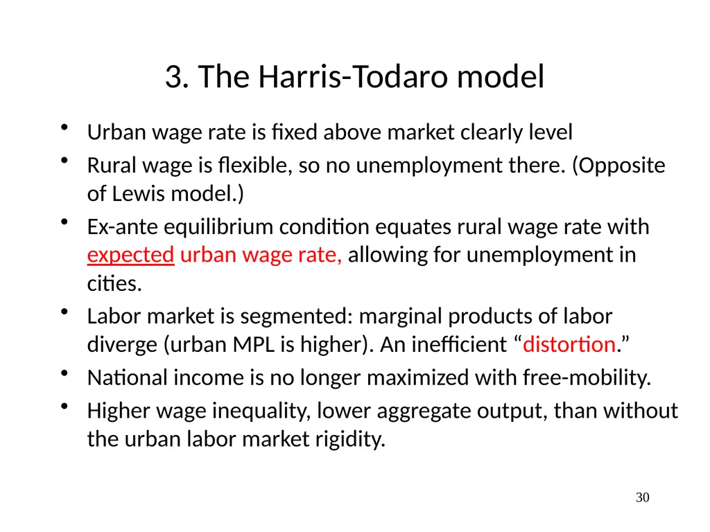
slide30. 3. The Harris-Todaro model Urban wage rate is fixed above market clearly level
Rural wage is flexible, so no unemployment there. (Opposite of Lewis model.)
Ex-ante equilibrium condition equates rural wage rate with expected urban wage rate, allowing for unemployment in cities.
Labor market is segmented: marginal products of labor diverge (urban MPL is higher). An inefficient “distortion.”
National income is no longer maximized with free-mobility.
Higher wage inequality, lower aggregate output, than without the urban labor market rigidity. 30<br>
slide31. Why is the urban wage sticky downwards? Easier for urban workers to organize as a trade union, and bid up their wage rate.
Easier to enforce a statutory minimum wage rate in urban areas (though still limits to compliance).
Urban firms may tend to use technologies with higher monitoring costs. Firms then choose to pay a premium to avoid shirking.
Cities as the “show case”: extra benefits (such as from government) make an urban job more attractive even if the wage rate is similar. 31<br>
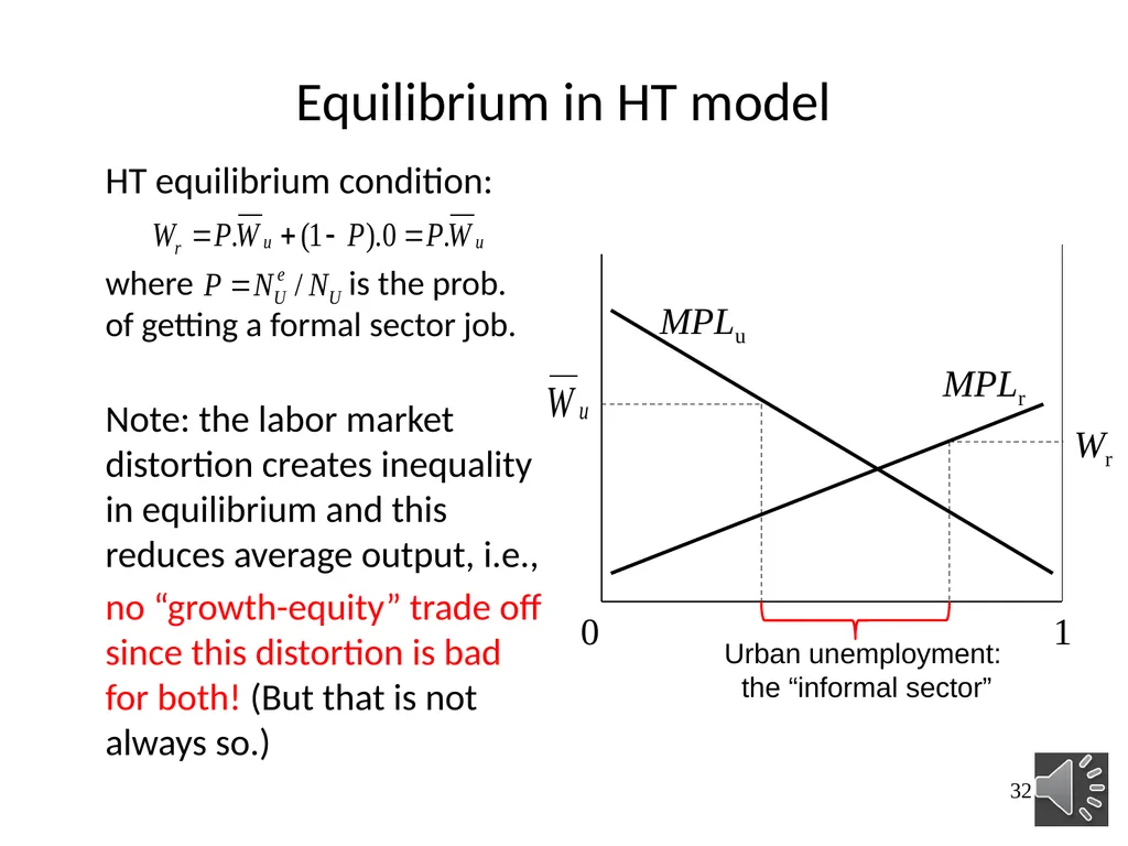
slide32. Equilibrium in HT model HT equilibrium condition:

where is the prob. of getting a formal sector job.

Note: the labor market distortion creates inequality in equilibrium and this reduces average output, i.e.,
no “growth-equity” trade off since this distortion is bad for both! (But that is not always so.) 32 MPLu MPLr 0 1 Wr Urban unemployment:
the “informal sector”<br>
slide33. What happens to the unemployment rate? Govt. jobs program initially reduces urban unemployment rate.
But this attracts rural migrants, not all of whom get a job.
With fewer rural workers the rural wage rises.
Two opposing forces: number of unemployed need not fall once equilibrium is restored.
Depends on specifics of the setting (labor demand functions). 33 MPLu MPLr 0 1 Wr But then rises back toward
the old level Urban unemployment
initially shrinks<br>
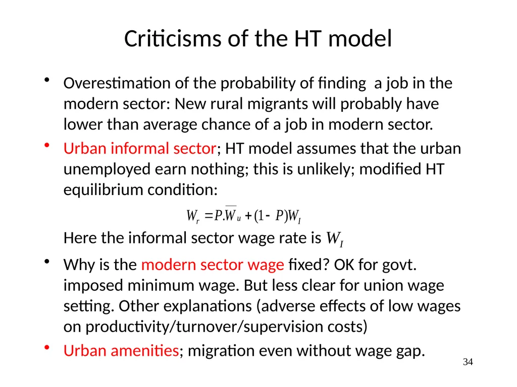
slide34. Criticisms of the HT model Overestimation of the probability of finding a job in the modern sector: New rural migrants will probably have lower than average chance of a job in modern sector.
Urban informal sector; HT model assumes that the urban unemployed earn nothing; this is unlikely; modified HT equilibrium condition:

Here the informal sector wage rate is WI
Why is the modern sector wage fixed? OK for govt. imposed minimum wage. But less clear for union wage setting. Other explanations (adverse effects of low wages on productivity/turnover/supervision costs)
Urban amenities; migration even without wage gap. 34<br>
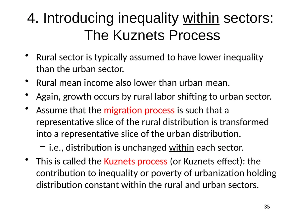
slide35. 35 4. Introducing inequality within sectors: The Kuznets Process Rural sector is typically assumed to have lower inequality than the urban sector.
Rural mean income also lower than urban mean.
Again, growth occurs by rural labor shifting to urban sector.
Assume that the migration process is such that a representative slice of the rural distribution is transformed into a representative slice of the urban distribution.
i.e., distribution is unchanged within each sector.
This is called the Kuznets process (or Kuznets effect): the contribution to inequality or poverty of urbanization holding distribution constant within the rural and urban sectors.<br>
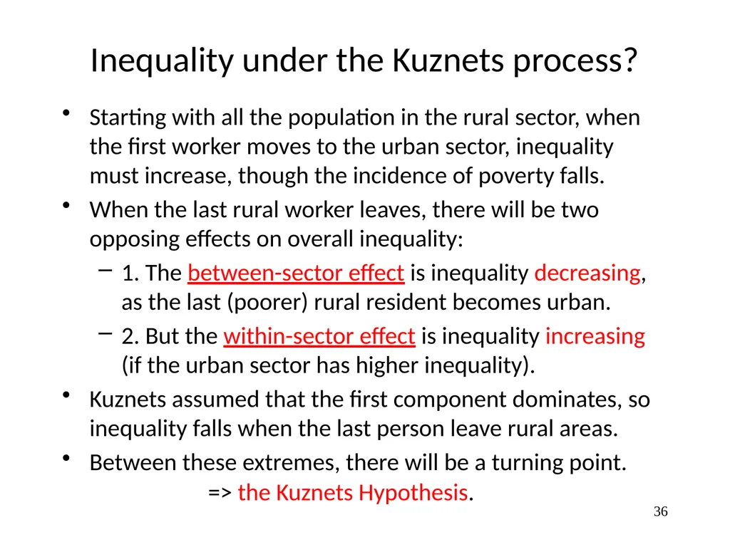
slide36. Inequality under the Kuznets process? Starting with all the population in the rural sector, when the first worker moves to the urban sector, inequality must increase, though the incidence of poverty falls.
When the last rural worker leaves, there will be two opposing effects on overall inequality:
1. The between-sector effect is inequality decreasing, as the last (poorer) rural resident becomes urban.
2. But the within-sector effect is inequality increasing (if the urban sector has higher inequality).
Kuznets assumed that the first component dominates, so inequality falls when the last person leave rural areas.
Between these extremes, there will be a turning point.
=> the Kuznets Hypothesis. 36<br>
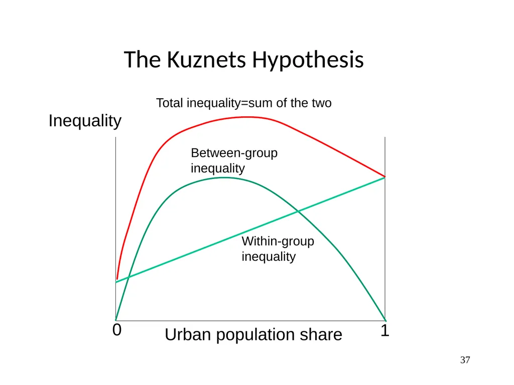
slide37. The Kuznets Hypothesis 37 Inequality 0 1 Between-group
inequality Within-group
inequality Urban population share Total inequality=sum of the two<br>
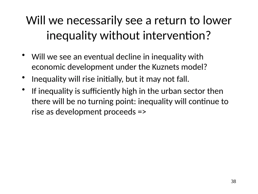
slide38. 38 Will we necessarily see a return to lower inequality without intervention? Will we see an eventual decline in inequality with economic development under the Kuznets model?
Inequality will rise initially, but it may not fall.
If inequality is sufficiently high in the urban sector then there will be no turning point: inequality will continue to rise as development proceeds =><br>
slide39. If urban inequality is high enough then we will not see the inverted U 39 Inequality 0 1 Between-
group Within-
group Urban population share Total inequality<br>
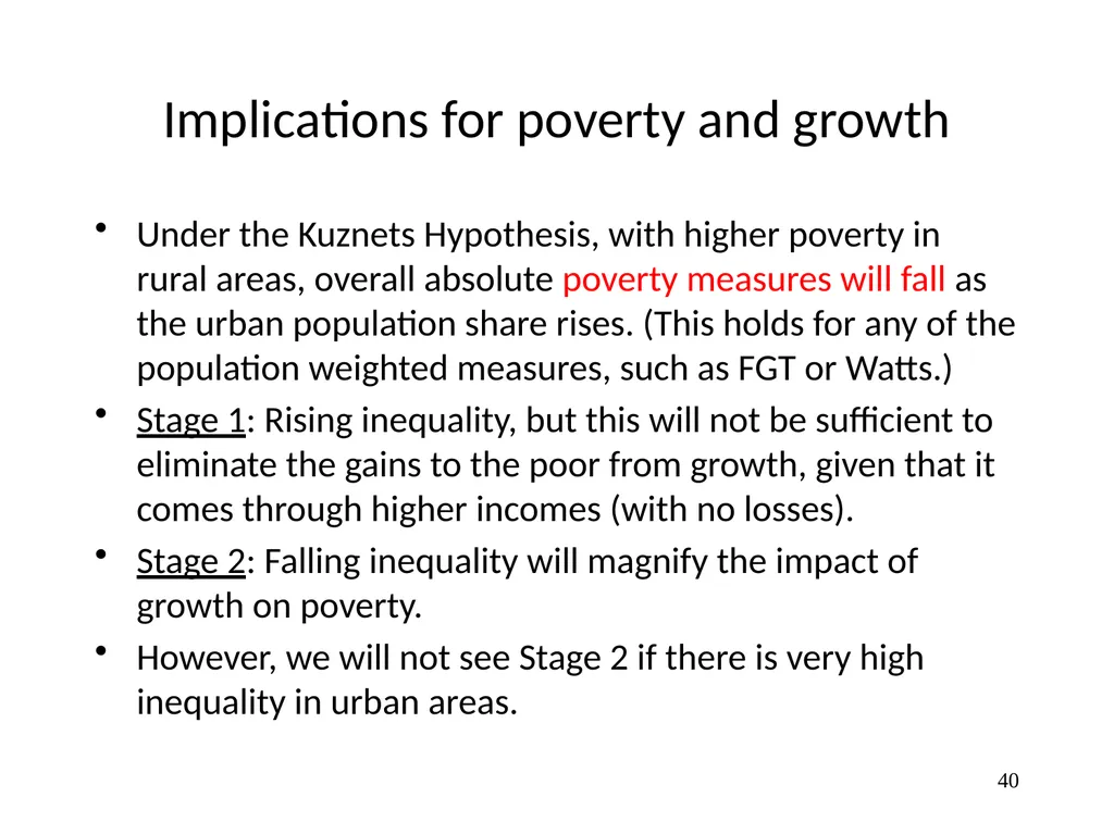
slide40. 40 Implications for poverty and growth Under the Kuznets Hypothesis, with higher poverty in rural areas, overall absolute poverty measures will fall as the urban population share rises. (This holds for any of the population weighted measures, such as FGT or Watts.)
Stage 1: Rising inequality, but this will not be sufficient to eliminate the gains to the poor from growth, given that it comes through higher incomes (with no losses).
Stage 2: Falling inequality will magnify the impact of growth on poverty.
However, we will not see Stage 2 if there is very high inequality in urban areas.<br>
slide41. 41 High poverty and inequality
=>Low growth?

Does inequality impede growth?
Does poverty impede growth?
Is poverty self-perpetuating?<br>
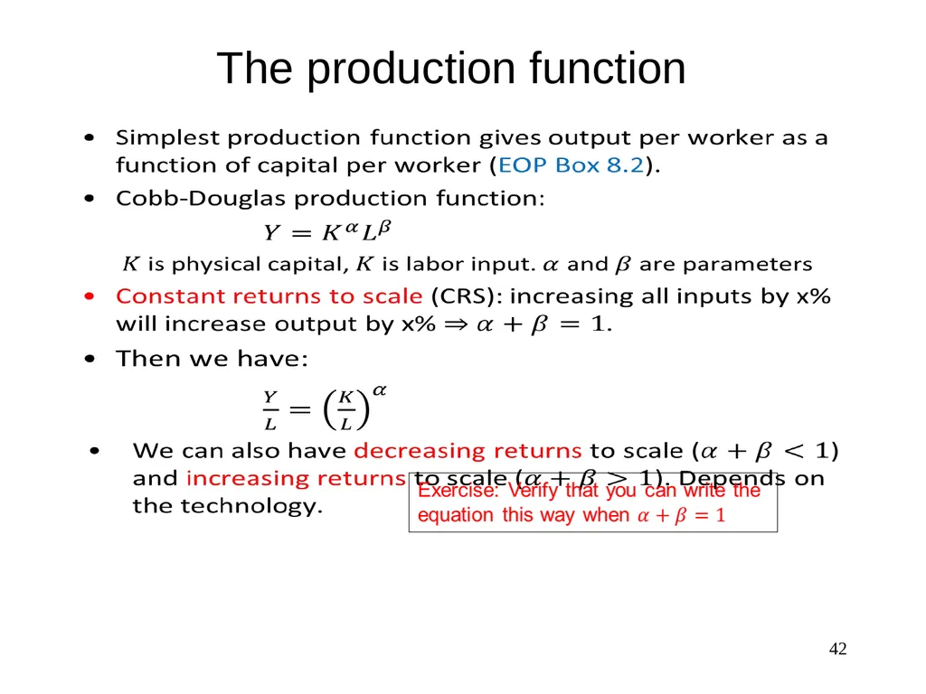
slide42. The production function 42<br>
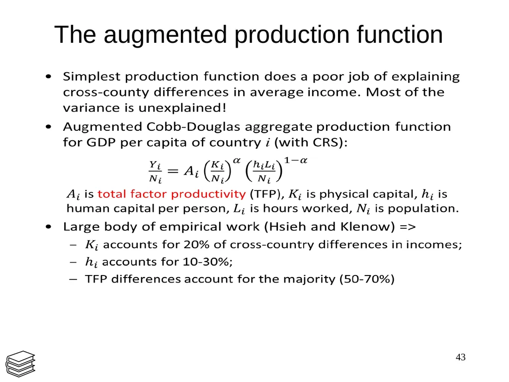
slide43. The augmented production function 43<br>
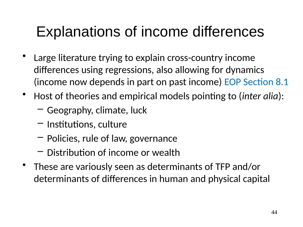
slide44. Explanations of income differences Large literature trying to explain cross-country income differences using regressions, also allowing for dynamics (income now depends in part on past income) EOP Section 8.1
Host of theories and empirical models pointing to (inter alia):
Geography, climate, luck
Institutions, culture
Policies, rule of law, governance
Distribution of income or wealth
These are variously seen as determinants of TFP and/or determinants of differences in human and physical capital 44<br>
slide45. Four ways that high inequality can impede growth 45<br>
slide46. 1. Failure to cooperate Inequality can generate social conflicts that restrict efficiency-enhancing cooperation amongst people.
such that public goods needed for growth are underprovided, or
efficiency-enhancing policy reforms are blocked by powerful elites. 46<br>
slide47. 2. Encouragement for wasteful policies High inequality can lead democratic governments to implement wasteful (“distortionary”) policies, which come at a cost to aggregate output and (hence) growth.
For example, higher inequality => a high mean relative to the median.
Then there will be stronger political support for redistribution from above the mean to below it, which may be costly to the economy as a whole.
However, the political-economy can change when there exist efficiency enhancing anti-poverty policies. Sipport emerges for pro-poor redistribution to enhance output. 47<br>
slide48. 3. Horizontal inequalities create frictions to efficiency Inequality of opportunity in society such as due to ethnic, racial or gender discrimination mean that some people are prevented from advancement, while otherwise identical people succeed.
This is a misallocation of talent leading to inefficiency.
Sandra Day O’Connor example: brilliant law student graduates (1952) but can only get a job as a legal secretary.
Overall output is lower than it would be without these horizontal inequalities.
One estimate: 40% of US economic growth since early 1950s is due to reduction in these inequalities (Hsieh et al.) Also, more gains ahead by removing these barriers. 48<br>
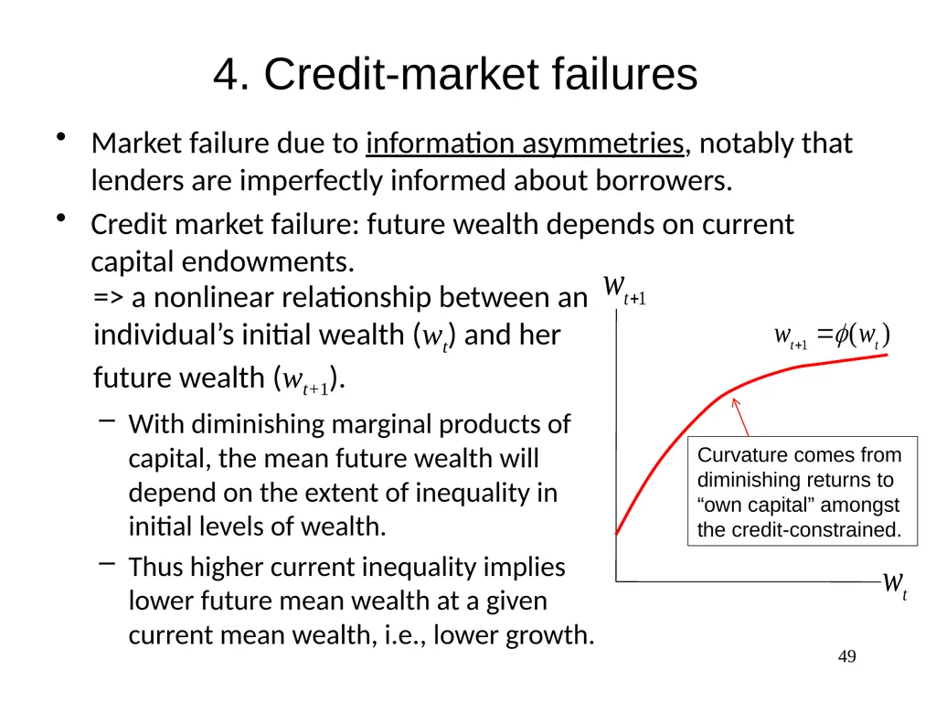
slide49. 4. Credit-market failures => a nonlinear relationship between an individual’s initial wealth (wt) and her future wealth (wt+1).
With diminishing marginal products of capital, the mean future wealth will depend on the extent of inequality in initial levels of wealth.
Thus higher current inequality implies lower future mean wealth at a given current mean wealth, i.e., lower growth. 49 Market failure due to information asymmetries, notably that lenders are imperfectly informed about borrowers.
Credit market failure: future wealth depends on current capital endowments. Curvature comes from
diminishing returns to
“own capital” amongst
the credit-constrained.<br>
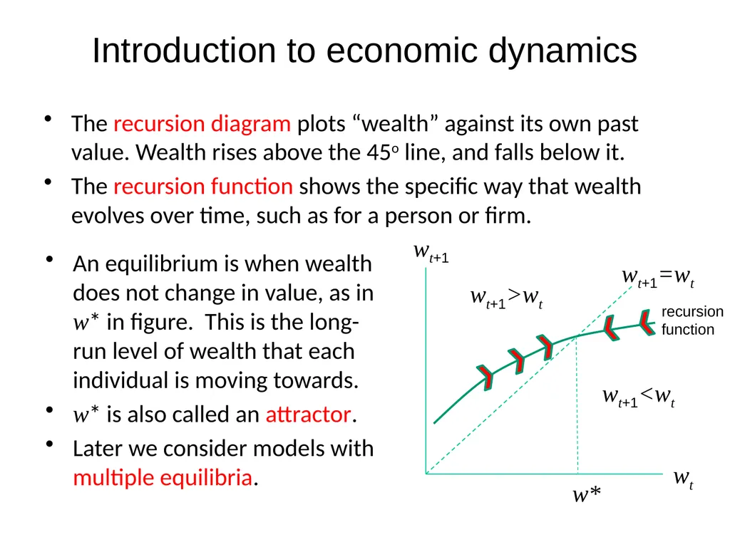
slide50. Introduction to economic dynamics The recursion diagram plots “wealth” against its own past value. Wealth rises above the 45o line, and falls below it.
The recursion function shows the specific way that wealth evolves over time, such as for a person or firm. wt+1 wt+1=wt w* wt An equilibrium is when wealth does not change in value, as in w* in figure. This is the long-run level of wealth that each individual is moving towards.
w* is also called an attractor.
Later we consider models with multiple equilibria. wt+1>wt wt+1<wt recursion function<br>
slide51. Four ways that poverty also impedes growth => poverty persists 51<br>
slide52. Poverty can impede growth and (hence) poverty reduction. Then poverty persists Four examples of how this can happen:
Early childhood underdevelopment
Impatience for current consumption
Technological progress
Credit market failures (again) 52<br>
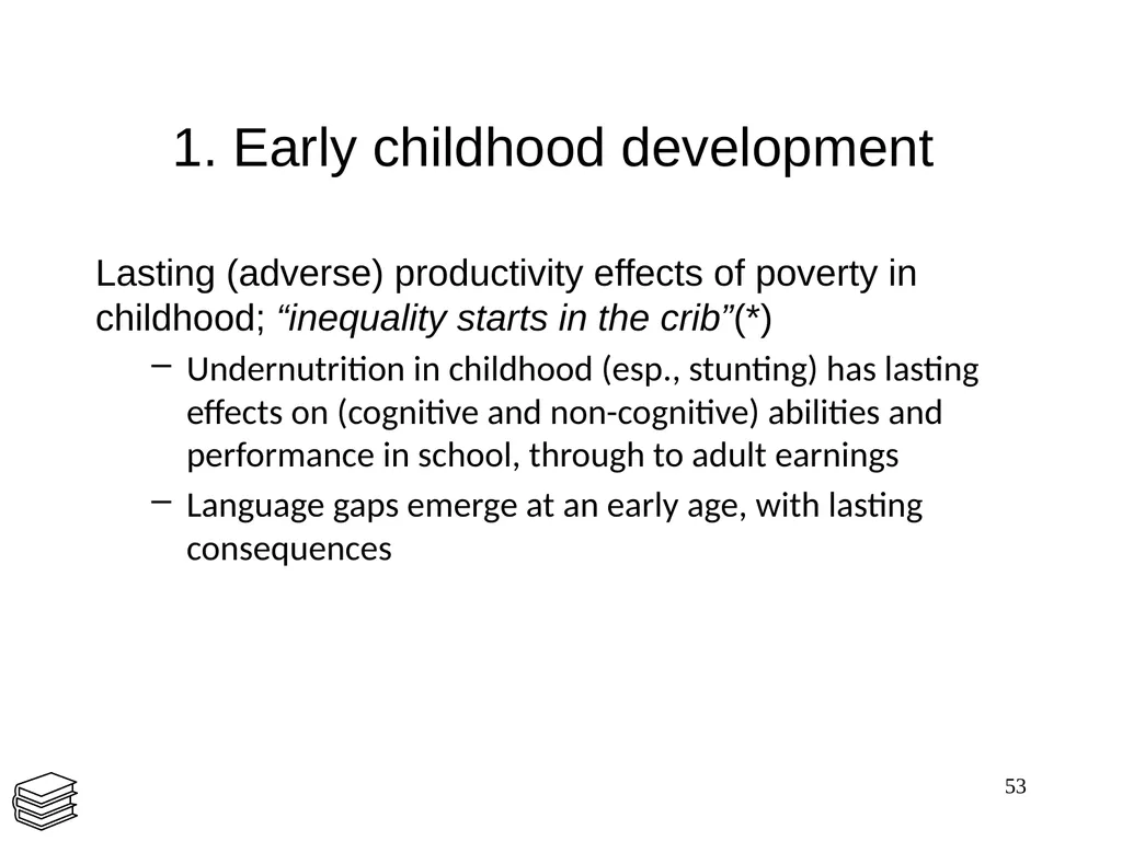
slide53. 1. Early childhood development Lasting (adverse) productivity effects of poverty in childhood; “inequality starts in the crib”(*)
Undernutrition in childhood (esp., stunting) has lasting effects on (cognitive and non-cognitive) abilities and performance in school, through to adult earnings
Language gaps emerge at an early age, with lasting consequences 53<br>
slide54. 2. Impatience Poverty compels a person to put high weight on current consumption relative to future consumption.
This is called a high discount rate (or “rate of time preference”)
This can be understood in terms of the economics of inter-temporal consumer choice (savings).
Thus poorer person today invests less, thus seeing less future income growth => more likely to stay poor. 54<br>
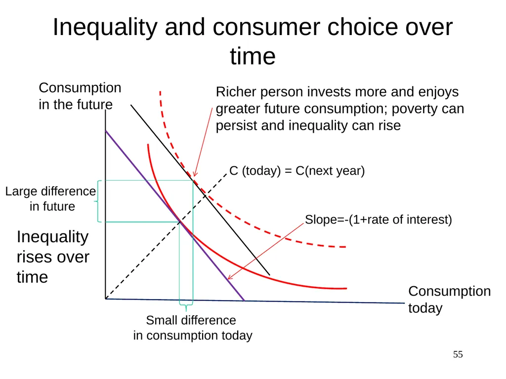
slide55. Inequality and consumer choice over time 55 Consumption in the future Richer person invests more and enjoys greater future consumption; poverty can persist and inequality can rise Consumption today C (today) = C(next year) Small difference
in consumption today Large difference
in future Slope=-(1+rate of interest) Inequality
rises over
time<br>
slide56. 3. Knowledge and technical progress Technical (=“technological”) progress = producing more from given capital and labor.
High levels of knowledge, starting with educational investments, create the potential to invent new ways of doing things, i.e., technical progress.
Knowledge is produced, but it has some special features.
Knowledge is not likely to have diminished returns (as in Ricardo). Knowing more makes it easier to learn more.
Some producers will become dominant in the market, esp., if they can protect their inventions.
Against this, spillover effects may be hard to avoid, making it harder for monopolies to form. 56<br>
slide57. Technical progress and poverty Poverty inhibits human capital investments, reducing the scope for home-grown technical progress.
Thus we can understand why we tend to see more technical innovation in rich countries than poor ones.
Copying foreign technologies through trade may help.
However, the technologies available in rich countries may not be appropriate for poor, technology-importing, countries. They need home-grown methods.
Thus (again) poverty can handicap growth prospects.
Even so, there can still be ample scope for doing better in producing more with given technologies, and catching up.
Investments in human capital along the way will be key. 57<br>
slide58. 4. Borrowing constraints Credit market failures have lasting consequences for pro-poor growth
Those with sufficient wealth will reach their unconstrained optimum, equating the marginal product of capital with the interest rate.
But the “wealth poor,” for whom the borrowing constraint is binding, will not be able to do so.
Higher current wealth poverty for a given mean also implies lower growth.
More poverty initially implies more credit-constrained people, and (hence) less investment and growth. 58<br>
slide59. Poverty can also be the cause of market failure When a person is close to the lowest possible utility, punishment incentives do not bite.
Thus, a poor person may have a hard time convincing lenders (and others) that she is trustworthy.
The credit market failure may thus stem from poverty itself. 59<br>
slide60. Poverty traps 60<br>
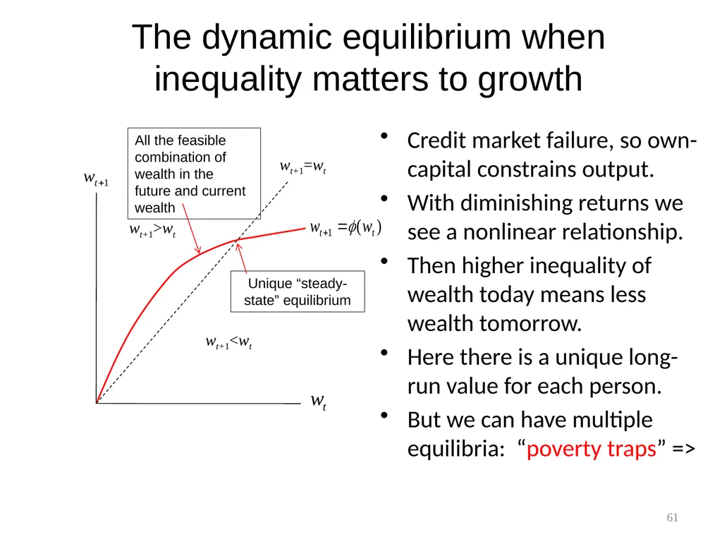
slide61. The dynamic equilibrium wheninequality matters to growth Credit market failure, so own-capital constrains output.
With diminishing returns we see a nonlinear relationship.
Then higher inequality of wealth today means less wealth tomorrow.
Here there is a unique long-run value for each person.
But we can have multiple equilibria: “poverty traps” => 61 wt+1=wt Unique “steady-state” equilibrium wt+1>wt wt+1<wt All the feasible combination of wealth in the future and current wealth<br>
slide62. Single vs multiple equilibria The model in the last slide has one unique equilibrium for each individual. (Also called a “steady-state equilibrium.”)
This is the individual’s long-run equilibrium, which she is moving toward.
This is stable, meaning that (without any assistance) wealth returns to that equilibrium after a shock.
Multiple equilibria—some stable some not—can arise when there is a threshold effect, i.e., a minimum level of wealth below which one cannot generate any future wealth.
Poverty traps can arise in such models. 62<br>
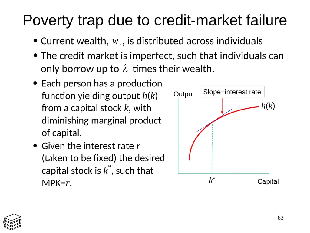
slide63. Poverty trap due to credit-market failure 63 Output Capital h(k) k* Slope=interest rate<br>
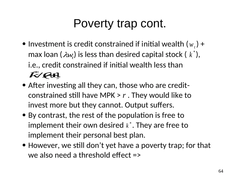
slide64. Poverty trap cont. 64<br>
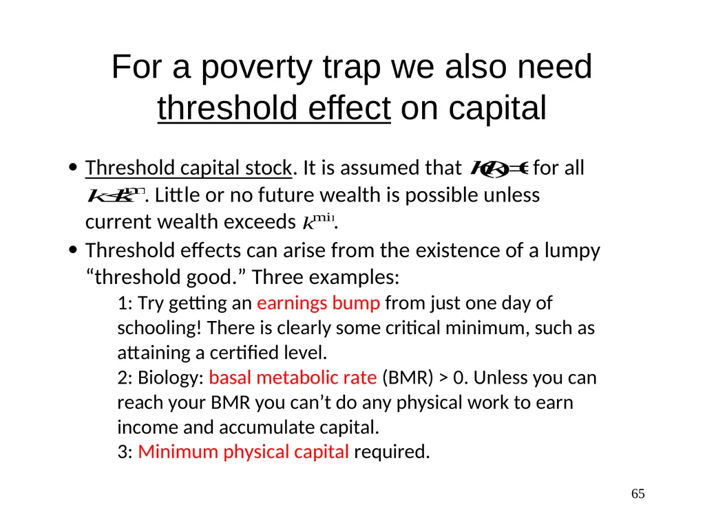
slide65. For a poverty trap we also need threshold effect on capital 65<br>
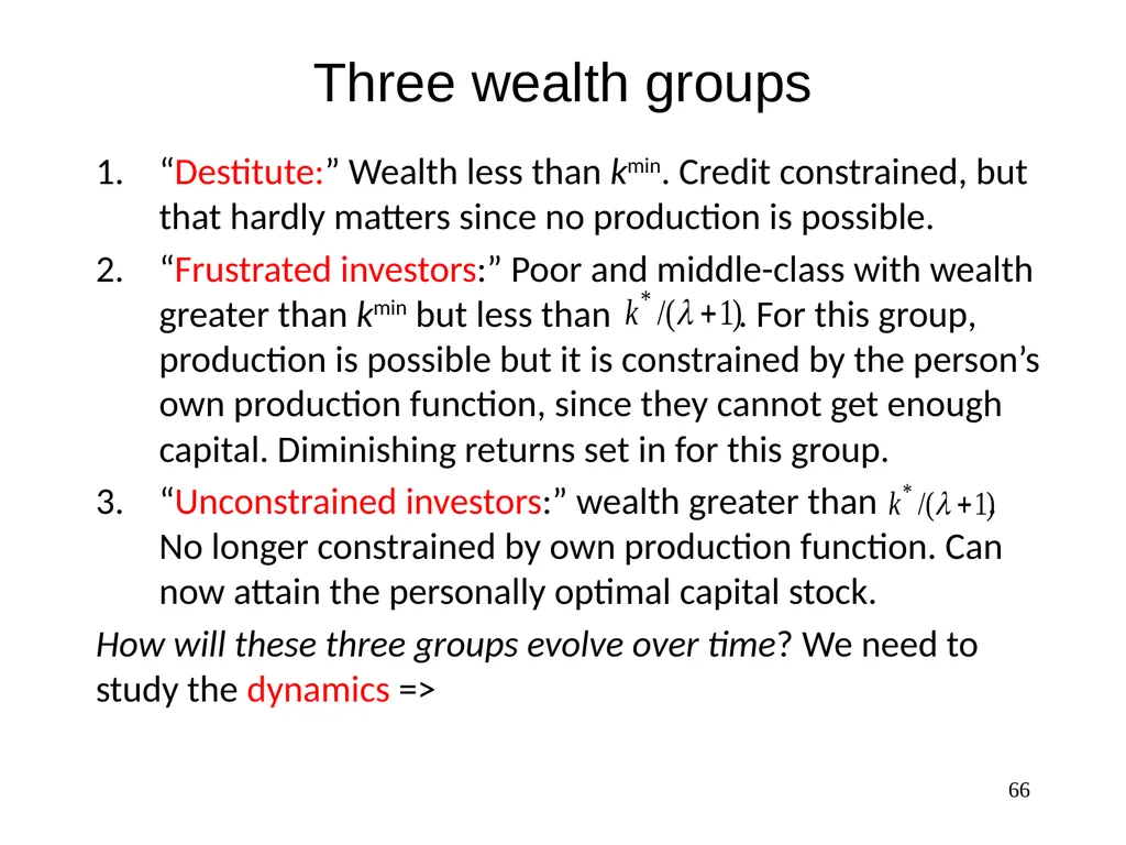
slide66. Three wealth groups “Destitute:” Wealth less than kmin. Credit constrained, but that hardly matters since no production is possible.
“Frustrated investors:” Poor and middle-class with wealth greater than kmin but less than . For this group, production is possible but it is constrained by the person’s own production function, since they cannot get enough capital. Diminishing returns set in for this group.
“Unconstrained investors:” wealth greater than . No longer constrained by own production function. Can now attain the personally optimal capital stock.
How will these three groups evolve over time? We need to study the dynamics => 66<br>
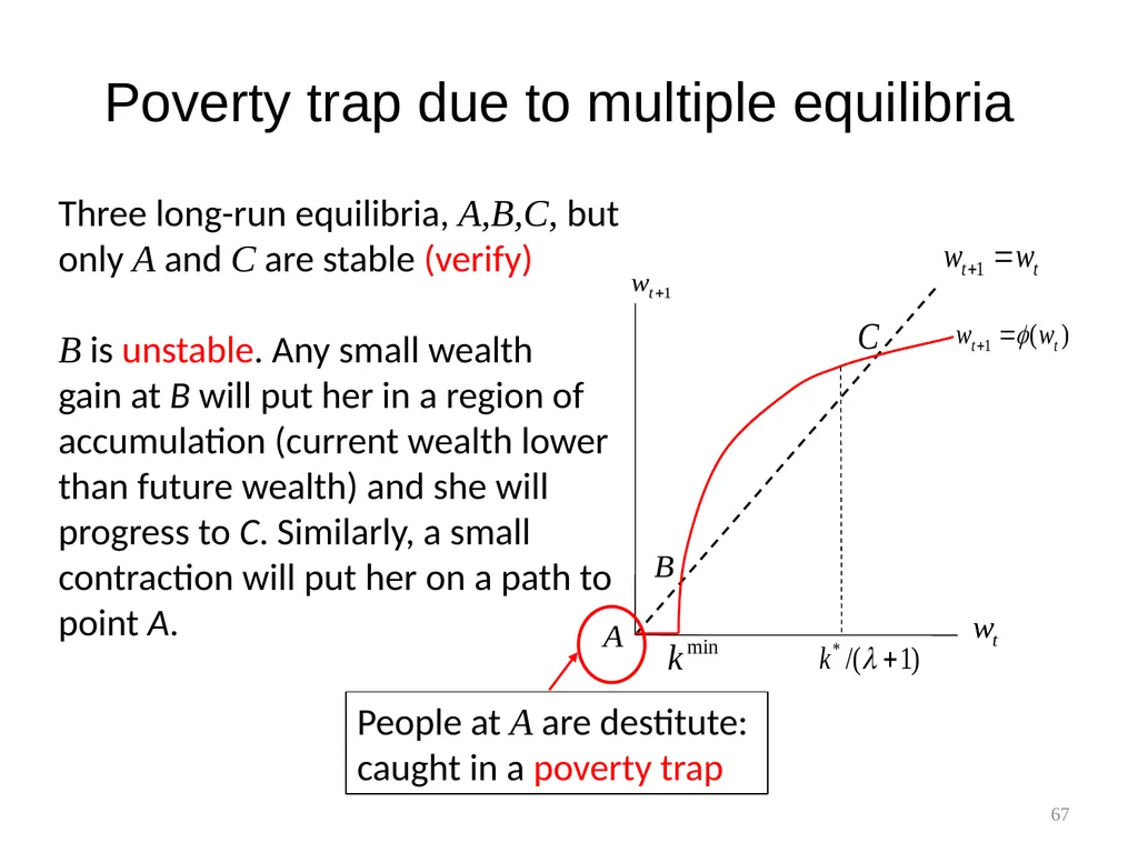
slide67. Poverty trap due to multiple equilibria 67 Three long-run equilibria, A,B,C, but only A and C are stable (verify)

B is unstable. Any small wealth
gain at B will put her in a region of accumulation (current wealth lower than future wealth) and she will progress to C. Similarly, a small contraction will put her on a path to point A. People at A are destitute:
caught in a poverty trap<br>
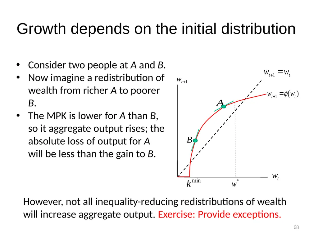
slide68. Growth depends on the initial distribution 68 Consider two people at A and B.
Now imagine a redistribution of wealth from richer A to poorer B.
The MPK is lower for A than B, so it aggregate output rises; the absolute loss of output for A will be less than the gain to B. However, not all inequality-reducing redistributions of wealth
will increase aggregate output. Exercise: Provide exceptions.<br>
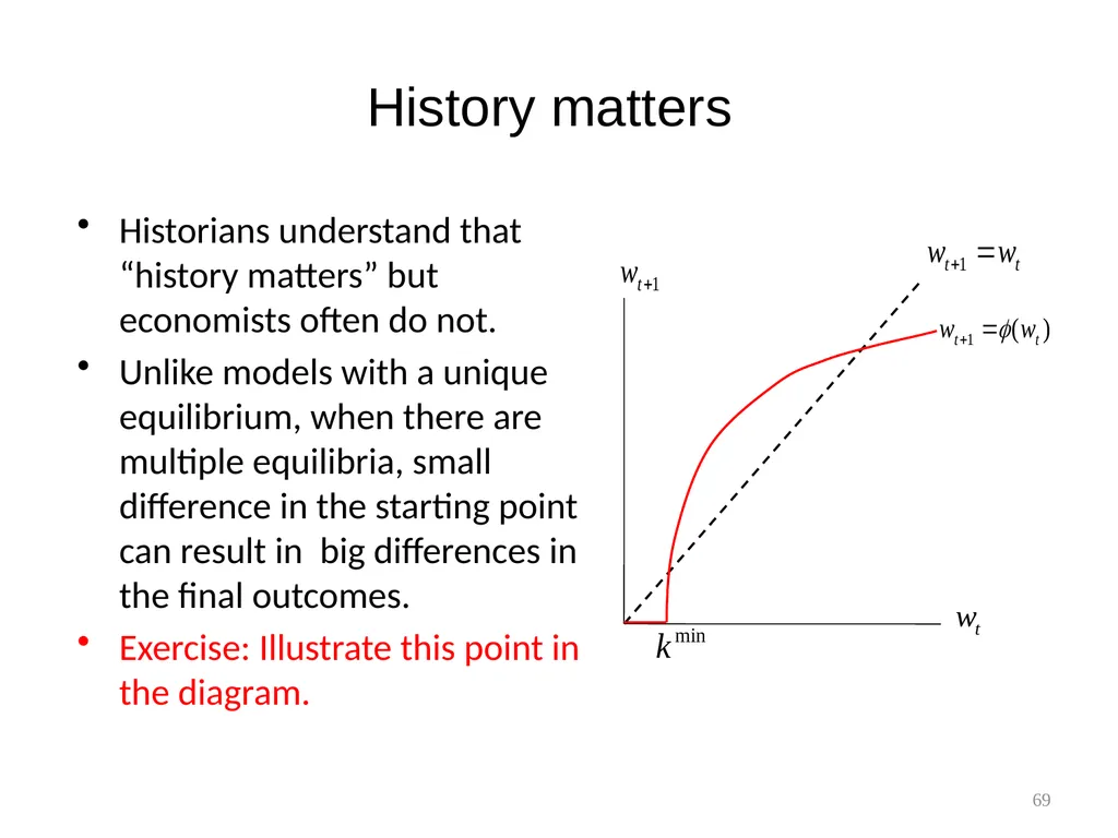
slide69. History matters Historians understand that “history matters” but economists often do not.
Unlike models with a unique equilibrium, when there are multiple equilibria, small difference in the starting point can result in big differences in the final outcomes.
Exercise: Illustrate this point in the diagram. 69<br>
slide70. Geography can also matter We often find poor people concentrated in certain places.
This may be a selection process (voluntary or not), leading to a geographic concentration of poor people.
Location can also have a causal role. Living in a poor place can reduce the productivity of your labor and capital, making it harder to escape poverty.
Then we have a geographic poverty trap. Comparing two people with the same personal capital and labor, the one living in the poorer place will see less growth in income and wealth.
Example: EOP Box 8.22 on China’s lagging poor areas. 70<br>
slide71. 71 2. Evidence from country experiences(EOP: Section 8.2) Does growth come with rising inequality?
Does growth reduce poverty?
Does high inequality and/or high poverty
impede growth?
What is happening to aggregate poverty
and inequality?<br>
slide72. The Industrial Revolution (IR) and poverty: Optimists and pessimists Recall from Part 1 that throughout the C19th, Classical and Marxist economists were pessimistic on the scope for poverty-reducing growth.
Little hope for rising real wages even with technical progress. From Smith (1776) to Wicksell (1901).
They saw abject poverty among the new urban working class of the industrial towns (e.g., Engels on Manchester).
These social critics did not have the right counterfactual, which was living conditions in rural areas. 72<br>
slide73. Meanwhile, back in the village Recall that in the neoclassical model, the migration to the cities will put upward pressure on wages in rural areas.
Little sign that this happened during the IR, but long lag in wage adjustment.
However, other factors were putting downward pressure on living conditions in rural areas.
Enclosure movement and Enclosure Acts forced land consolidation, rejecting small farmers from common land.
Life in the villages got progressively worse as people left--rural blight. 73<br>
slide74. Recall: Long lags in gains to the poor from IR Real wages did not rise much for many decades after the industrial revolution (IR) started (1760). 74 However, in due course, real wages (and nutritional status) in England improved markedly despite continuing population growth. Source: Robert Allen<br>
slide75. Recall: Why did real wages not rise faster in the wake of the Industrial Revolution? Labor-displacing technical progress? Jobs lost. Resistance from workers (Luddites).
Malthusian trap? Higher fertility with higher wages.
Labor surplus in rural areas? (Lewis model)
Low savings by workers? With workers too poor to save, the new investments could only be financed by high profits.
Once enough capital had accumulated real wages rose.
But with such a large number of poor, even a small savings rate by workers could have financed accumulation. Weak financial institutions were the root cause.
Falling food prices later in C19th (imports from America and Australia). Technical progress here too: refrigeration! 75<br>
slide76. What has happened to inequality in growing economies? 76<br>
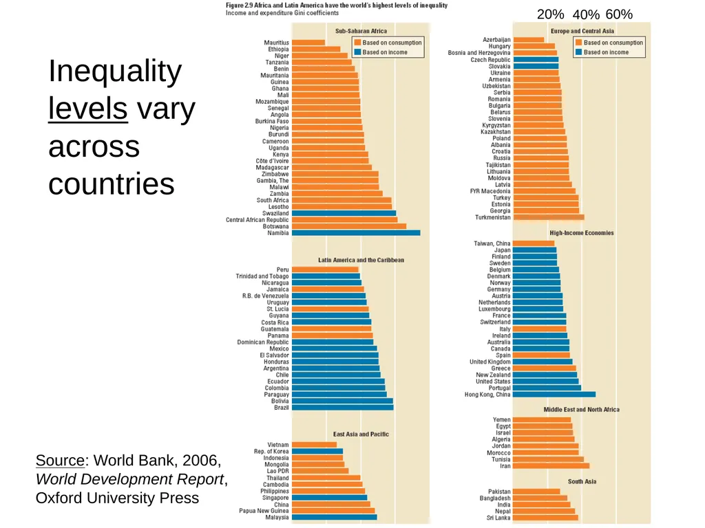
slide77. Inequality
levels vary across
countries Source: World Bank, 2006,
World Development Report,
Oxford University Press 20% 40% 60%<br>
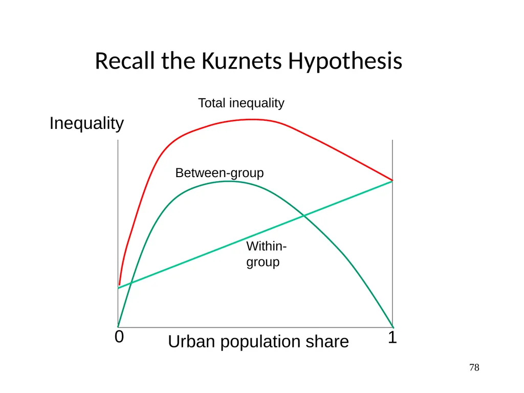
slide78. Recall the Kuznets Hypothesis 78 Inequality 0 1 Between-group Within-
group Urban population share Total inequality<br>
slide79. 79 Testing the Kuznets Hypothesis (KH) Past tests have looked at the cross-country relationship between inequality (typically Gini index) and GDP p.c. (call this Y) across countries.
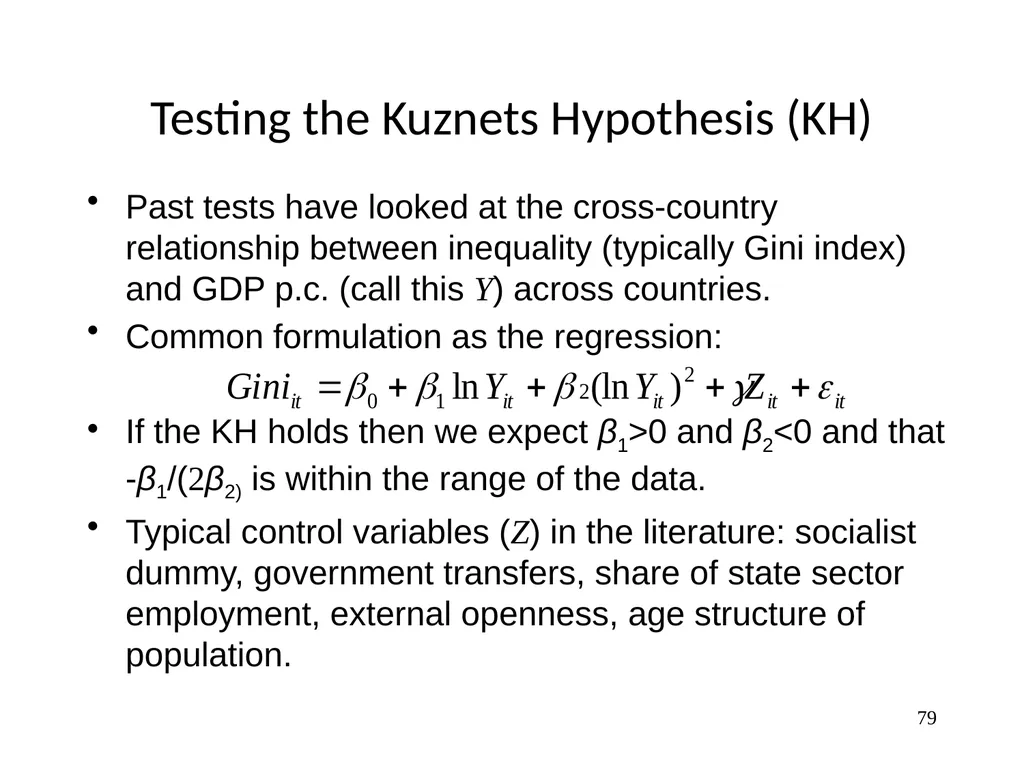
Common formulation as the regression:

If the KH holds then we expect β1>0 and β2<0 and that -β1/(2β2) is within the range of the data.
Typical control variables (Z) in the literature: socialist dummy, government transfers, share of state sector employment, external openness, age structure of population.<br>
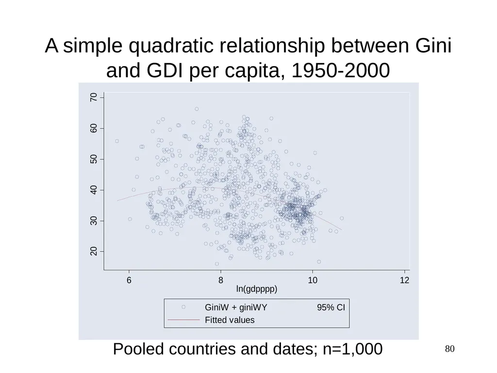
slide80. 80 A simple quadratic relationship between Gini and GDI per capita, 1950-2000 Pooled countries and dates; n=1,000<br>
slide81. 81 A weak inverted U relationship (more than 1000 Ginis)
Huge variability in inequality; R2 only 0.08
The upward sloping part of the curve is particularly hard to discern.
Turning point is quite unstable; here about $PPP 2,000 (level of Senegal).
Even this weak inverted U vanishes when we look at changes in both variables over time.

The most serious critique: With greater time series evidence, we find that very few developing countries have followed the prediction of the Kuznets Hypothesis.<br>
slide82. A closer look with more recent data 92 developing countries with at least two national surveys.
Longest spell between two surveys for each country.
Both surveys used the same welfare indicator, either consumption or income per person, following standard measurement practices.
Consumption was generally preferred. Three-quarters of the spells use consumption.
Comparability problems between surveys remain, such as differences in recall periods and imputation/valuation methods.
All changes between the surveys are annualized.
National accounts data were mapped as closely as possible to the survey dates, interpolating as need be.
All monetary measures are in constant 2005 prices (using country-specific Consumer Price Indices).
All international comparisons are at 2005 PPP. 82<br>
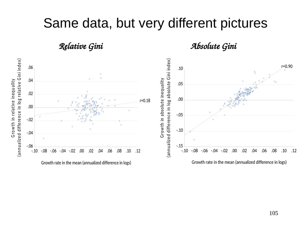
slide83. 83 Changes in relative inequality are only weakly correlated with growth 1. Across 144 spells (between two surveys), the correlation coefficient is 0.18 between changes in inequality (the log Gini index) and economic growth (change in the log of the survey mean or private consumption per capita from national accounts). Figure=>

2. Mean income of the poorest 20% (say) has a regression coefficient of about one on the overall growth rate.<br>
slide84. Inequality tends to rise with growth, though the effect is small 84<br>
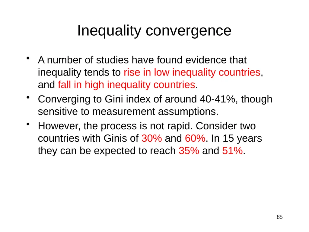
slide85. Inequality convergence A number of studies have found evidence that inequality tends to rise in low inequality countries, and fall in high inequality countries.
Converging to Gini index of around 40-41%, though sensitive to measurement assumptions.
However, the process is not rapid. Consider two countries with Ginis of 30% and 60%. In 15 years they can be expected to reach 35% and 51%. 85<br>
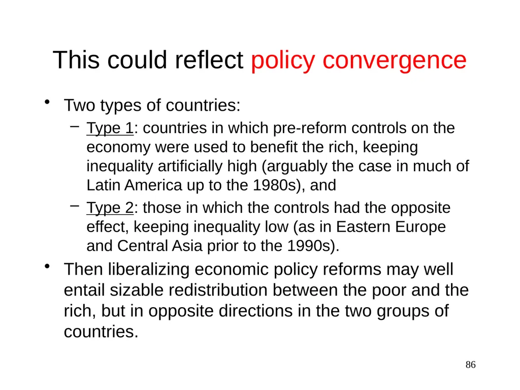
slide86. This could reflect policy convergence Two types of countries:
Type 1: countries in which pre-reform controls on the economy were used to benefit the rich, keeping inequality artificially high (arguably the case in much of Latin America up to the 1980s), and
Type 2: those in which the controls had the opposite effect, keeping inequality low (as in Eastern Europe and Central Asia prior to the 1990s).
Then liberalizing economic policy reforms may well entail sizable redistribution between the poor and the rich, but in opposite directions in the two groups of countries. 86<br>
slide87. Does growth reduce poverty? 87<br>
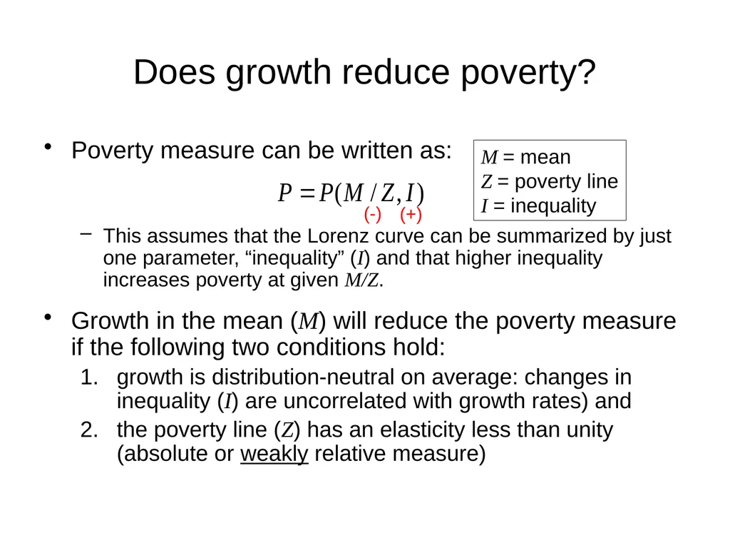
slide88. Does growth reduce poverty? Poverty measure can be written as:

This assumes that the Lorenz curve can be summarized by just one parameter, “inequality” (I) and that higher inequality increases poverty at given M/Z. M = mean
Z = poverty line
I = inequality (-) (+) Growth in the mean (M) will reduce the poverty measure if the following two conditions hold:
growth is distribution-neutral on average: changes in inequality (I) are uncorrelated with growth rates) and
the poverty line (Z) has an elasticity less than unity (absolute or weakly relative measure)<br>
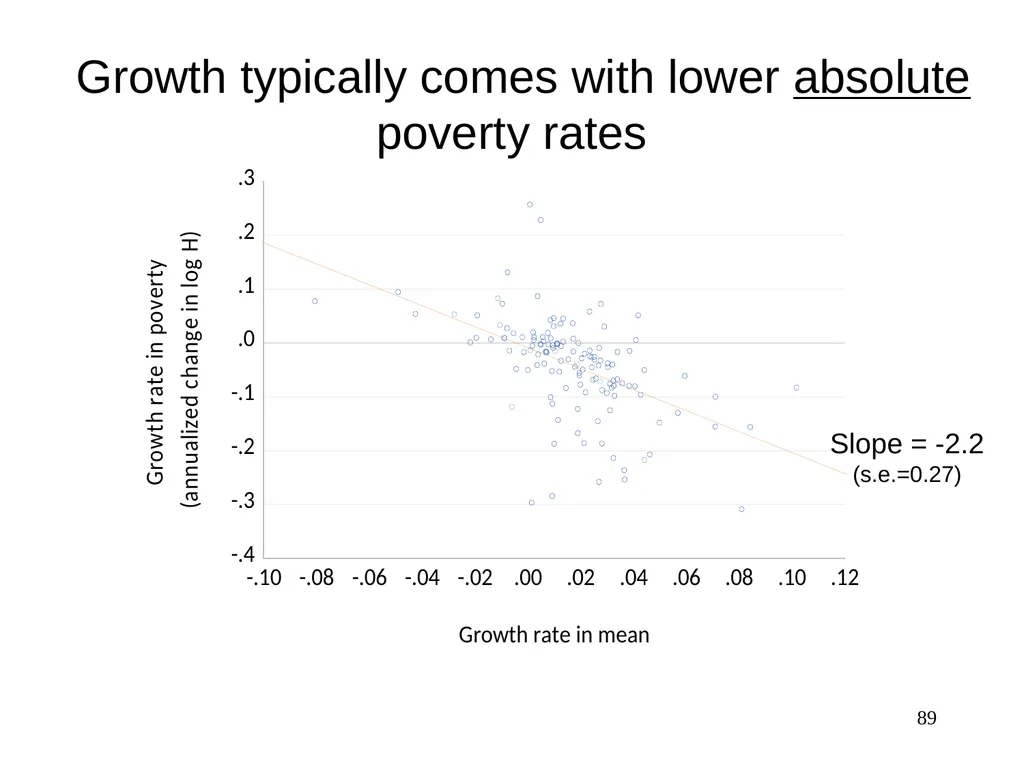
slide89. 89 Growth typically comes with lower absolute poverty rates Slope = -2.2
(s.e.=0.27)<br>
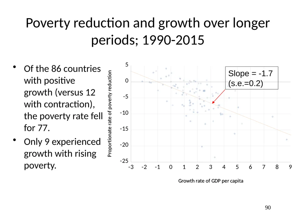
slide90. Poverty reduction and growth over longer periods; 1990-2015 Of the 86 countries with positive growth (versus 12 with contraction), the poverty rate fell for 77.
Only 9 experienced growth with rising poverty. 90 Slope = -1.7
(s.e.=0.2)<br>
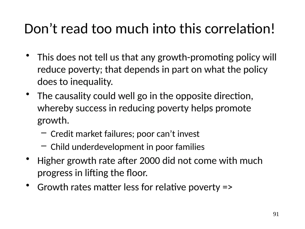
slide91. Don’t read too much into this correlation! This does not tell us that any growth-promoting policy will reduce poverty; that depends in part on what the policy does to inequality.
The causality could well go in the opposite direction, whereby success in reducing poverty helps promote growth.
Credit market failures; poor can’t invest
Child underdevelopment in poor families
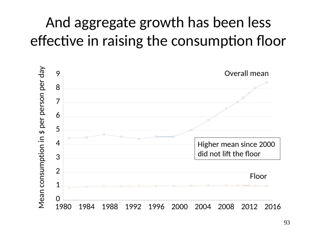
Higher growth rate after 2000 did not come with much progress in lifting the floor.
Growth rates matter less for relative poverty => 91<br>
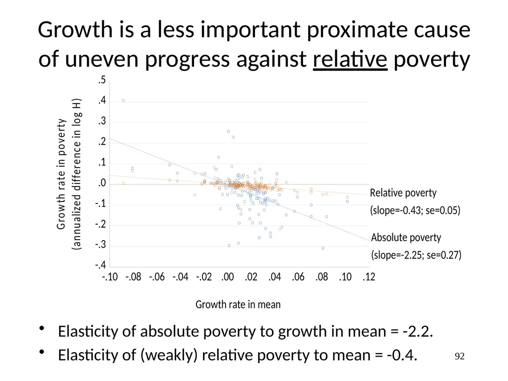
slide92. Growth is a less important proximate cause of uneven progress against relative poverty 92 Elasticity of absolute poverty to growth in mean = -2.2.
Elasticity of (weakly) relative poverty to mean = -0.4.<br>
slide93. And aggregate growth has been less effective in raising the consumption floor 93 Higher mean since 2000
did not lift the floor<br>
slide94. Largest absolute gains to the richAbsolute gains by percentile 1981-2011 94 “The worst-off benefit far more from trade than the rich.” (The Economist, October 2016)<br>
slide95. Does urbanization reduce poverty? 95<br>
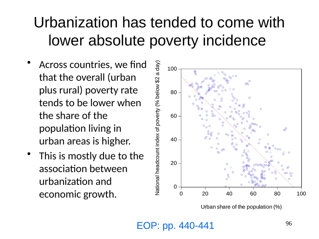
slide96. Urbanization has tended to come with lower absolute poverty incidence Across countries, we find that the overall (urban plus rural) poverty rate tends to be lower when the share of the population living in urban areas is higher.
This is mostly due to the association between urbanization and economic growth. 96 EOP: pp. 440-441<br>
slide97. Urbanization of poverty 1 Urban economic growth often provides new opportunities to rural out-migrants.
Winners and losers (Lectures for Part 3.1): Some migrants escape poverty in the process, though others may see little or no gain, and some of the rural migrants to urban areas may well end up worse off.
On average, there is likely to be a gain, otherwise migration will presumably cease.
But the overall gain to poor people, and falling national poverty rate, may well come with little or no progress against urban poverty. 97<br>
slide98. Urbanization of poverty 2 Important second-round impacts of urbanization on the living standards of those who remain in rural areas, notably through:
higher remittances from urban areas
the fact that there are fewer people competing for the available employment in rural areas.
Indeed, population urbanization has probably done more to reduce rural poverty than urban poverty!
However, mitigating forces, such as rural blight. 98<br>
slide99. Why has growth had such different outcomes for poor people? 99<br>
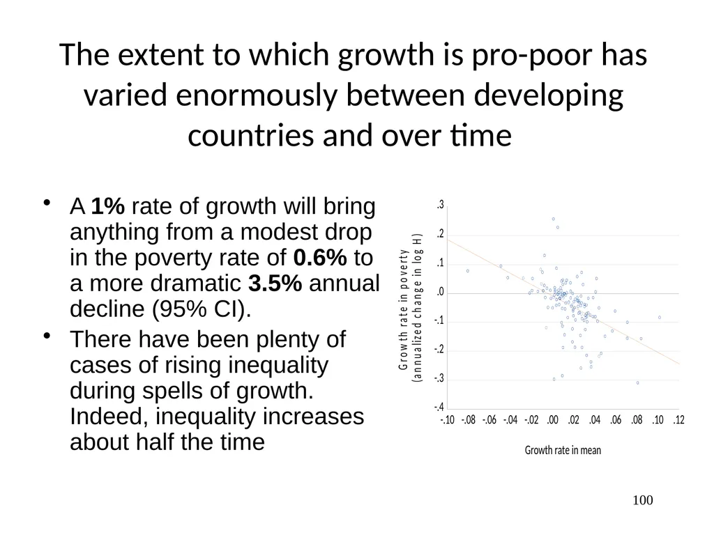
slide100. 100 The extent to which growth is pro-poor has varied enormously between developing countries and over time A 1% rate of growth will bring anything from a modest drop in the poverty rate of 0.6% to a more dramatic 3.5% annual decline (95% CI).
There have been plenty of cases of rising inequality during spells of growth. Indeed, inequality increases about half the time<br>
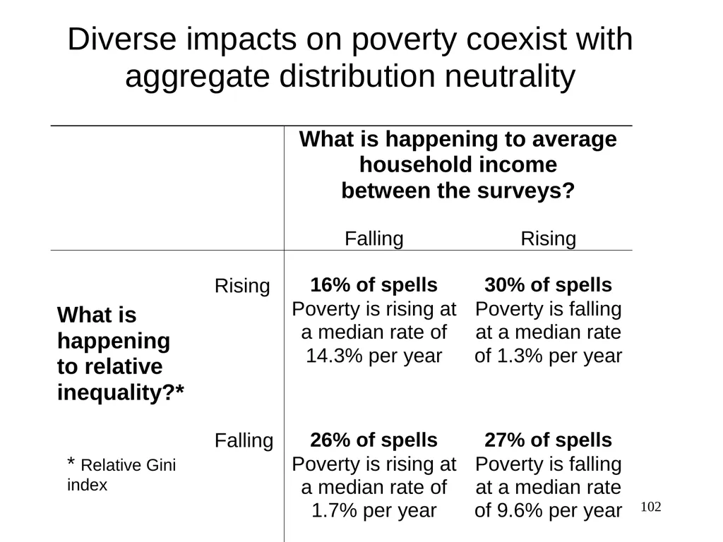
slide101. 101 Distribution-neutrality on average does not mean that distribution is unchanging In fact, measured inequality changes a lot during spells of growth, in both direction.
Large fluctuations in measured inequality even when there is no long-run trend
Some of this is measurement error; noise in inequality data
But even seemingly small changes in a Gini index (say) can mean large welfare changes for the poor<br>
slide102. 102<br>
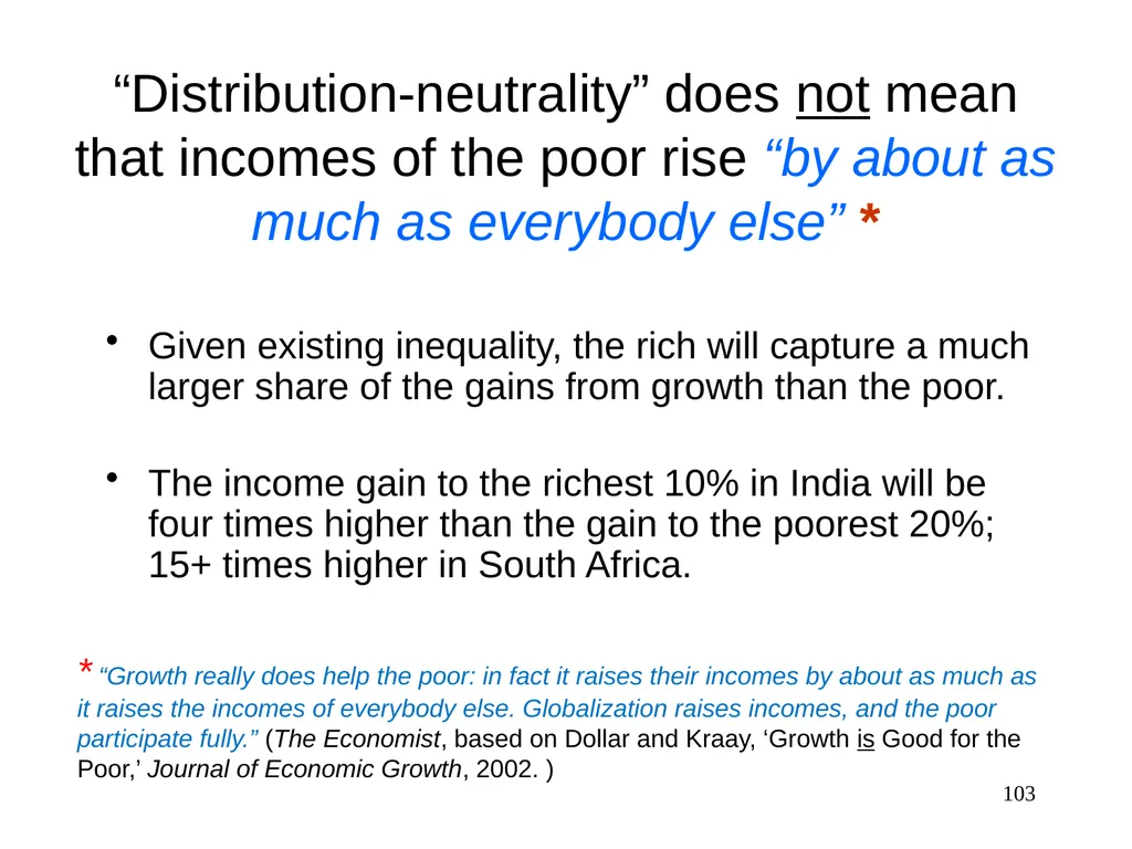
slide103. 103 “Distribution-neutrality” does not mean that incomes of the poor rise “by about as much as everybody else” * Given existing inequality, the rich will capture a much larger share of the gains from growth than the poor.

The income gain to the richest 10% in India will be four times higher than the gain to the poorest 20%; 15+ times higher in South Africa. * “Growth really does help the poor: in fact it raises their incomes by about as much as it raises the incomes of everybody else. Globalization raises incomes, and the poor participate fully.” (The Economist, based on Dollar and Kraay, ‘Growth is Good for the Poor,’ Journal of Economic Growth, 2002. )<br>
slide104. 104<br>
slide105. 105 Absolute Gini Relative Gini Same data, but very different pictures<br>
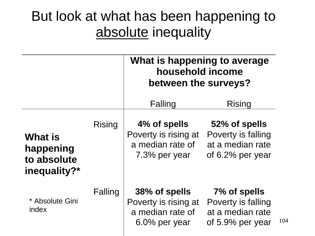
slide106. Differing concepts of “inequality” underlie policy debates, not differences in data Economists have traditionally focused on relative inequality. Mixed evidence, but distribution neutrality overall is still a plausible stylized fact.
However, a great many people focus instead on absolute disparities, which they see rising with growth.
One is not right and the other wrong: they are different concepts.
This must be recognized in the debate. 106<br>
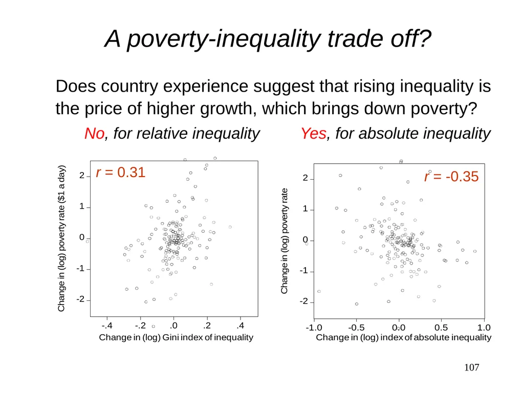
slide107. 107 A poverty-inequality trade off? Does country experience suggest that rising inequality is the price of higher growth, which brings down poverty?
No, for relative inequality Yes, for absolute inequality r = 0.31 r = -0.35<br>
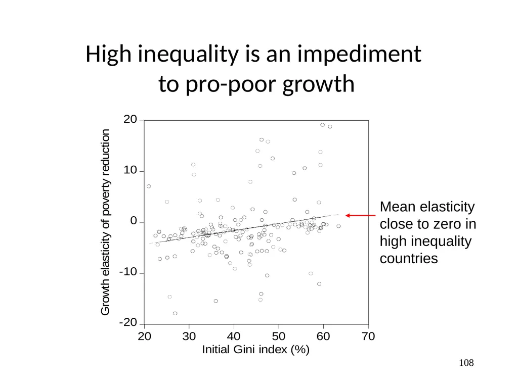
slide108. 108 High inequality is an impediment to pro-poor growth Mean elasticity
close to zero in
high inequality
countries<br>
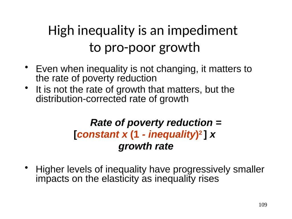
slide109. 109 High inequality is an impediment to pro-poor growth Even when inequality is not changing, it matters to the rate of poverty reduction
It is not the rate of growth that matters, but the distribution-corrected rate of growth Rate of poverty reduction =
[constant x (1 - inequality)2 ] x
growth rate

Higher levels of inequality have progressively smaller impacts on the elasticity as inequality rises<br>
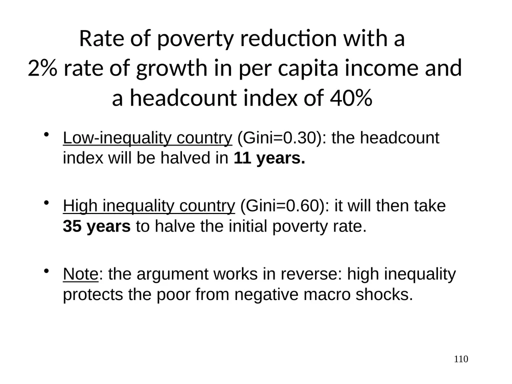
slide110. 110 Rate of poverty reduction with a 2% rate of growth in per capita income and a headcount index of 40% Low-inequality country (Gini=0.30): the headcount index will be halved in 11 years.

High inequality country (Gini=0.60): it will then take 35 years to halve the initial poverty rate.

Note: the argument works in reverse: high inequality protects the poor from negative macro shocks.<br>
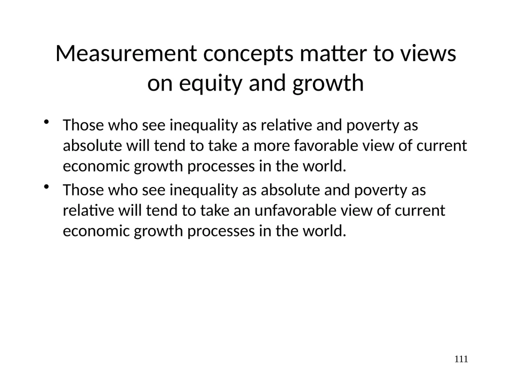
slide111. Measurement concepts matter to views on equity and growth Those who see inequality as relative and poverty as absolute will tend to take a more favorable view of current economic growth processes in the world.
Those who see inequality as absolute and poverty as relative will tend to take an unfavorable view of current economic growth processes in the world. 111<br>
slide112. 112 The US: A case study of rising inequality<br>
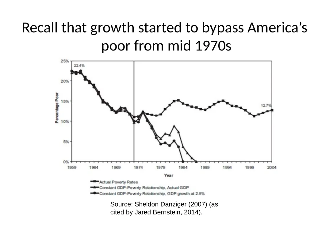
slide113. Source: Sheldon Danziger (2007) (as cited by Jared Bernstein, 2014). Recall that growth started to bypass America’s
poor from mid 1970s<br>
slide114. Why the rise in inequality and slow progress against poverty in the U.S.? Higher returns to schooling
Change in education policy in the 1970s that meant that the growth of skilled labor was not keeping up with the demand (Goldin and Katz). Rising skill premium.
Reinforced by changes in technology (skill-biased technical change) and de-unionization (weakening bargaining power).
The re-emergence of high rates of return to capital (relative to the growth rate) and greater industrial concentration—heading towards the rates of return to capital and profit rates that had not been seen since the early 20th century (Piketty). 114<br>
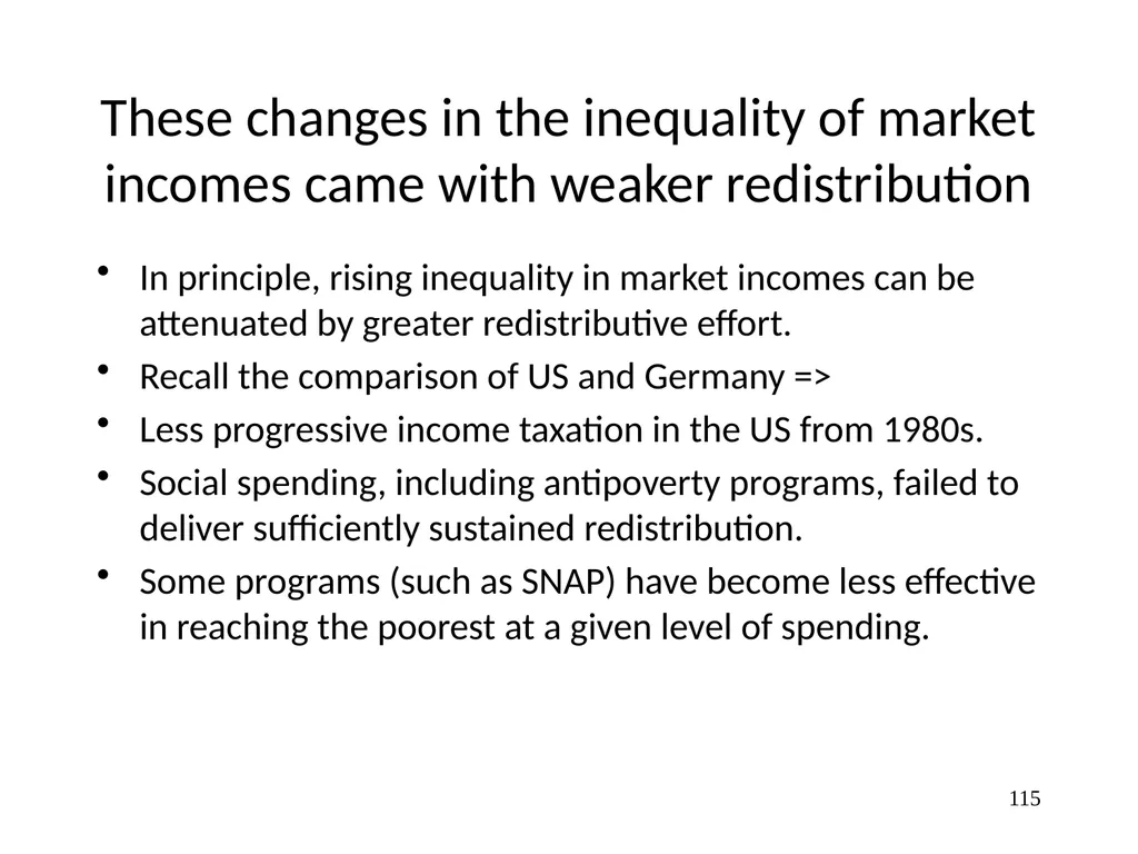
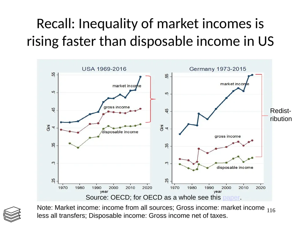
slide115. These changes in the inequality of market incomes came with weaker redistribution In principle, rising inequality in market incomes can be attenuated by greater redistributive effort.
Recall the comparison of US and Germany =>
Less progressive income taxation in the US from 1980s.
Social spending, including antipoverty programs, failed to deliver sufficiently sustained redistribution.
Some programs (such as SNAP) have become less effective in reaching the poorest at a given level of spending. 115<br>
slide116. Recall: Inequality of market incomes is rising faster than disposable income in US 116 Redist-
ribution Note: Market income: income from all sources; Gross income: market income less all transfers; Disposable income: Gross income net of taxes. Source: OECD; for OECD as a whole see this paper.<br>
slide117. 117 Does high inequality and/or high
poverty impede growth?
(EOP: Section 8.3)<br>
slide118. Past evidence on growth and inequality Empirical support from cross-country growth regressions for the view that higher inequality impedes growth.
Recent IMF research:
more unequal countries tend to have less sustained spells of growth, and this effect is also quite large;
higher initial inequality => countries redistribute more;
lower (post-tax) inequality yields higher growth and more long-lasting spells of growth;
redistribution is generally benign with regard to growth; it takes quite high levels of redistribution before any sign emerges of an adverse impact. 118<br>
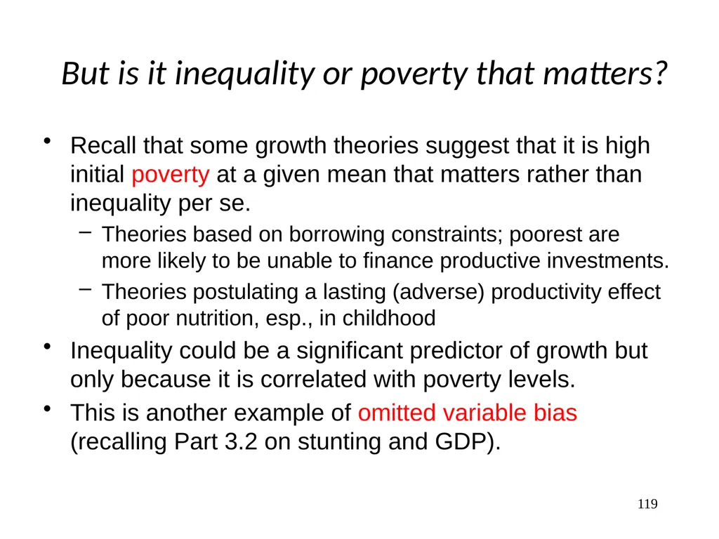
slide119. But is it inequality or poverty that matters? Recall that some growth theories suggest that it is high initial poverty at a given mean that matters rather than inequality per se.
Theories based on borrowing constraints; poorest are more likely to be unable to finance productive investments.
Theories postulating a lasting (adverse) productivity effect of poor nutrition, esp., in childhood
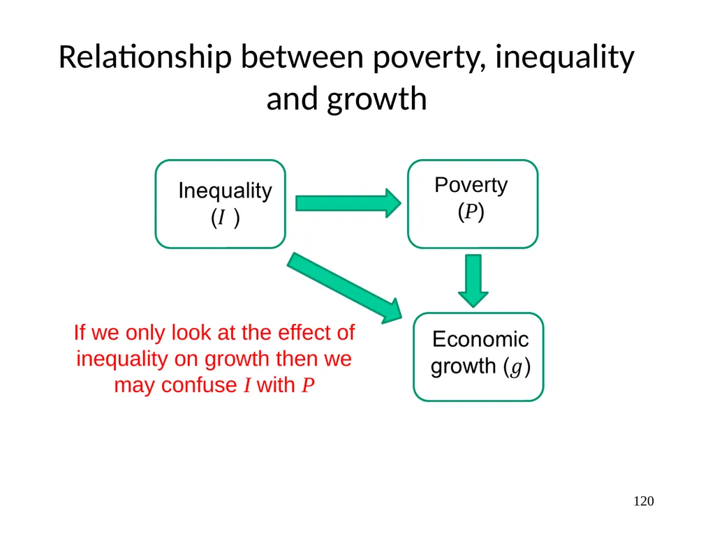
Inequality could be a significant predictor of growth but only because it is correlated with poverty levels.
This is another example of omitted variable bias (recalling Part 3.2 on stunting and GDP). 119<br>
slide120. Relationship between poverty, inequality and growth 120 Poverty
(P) If we only look at the effect of inequality on growth then we may confuse I with P<br>
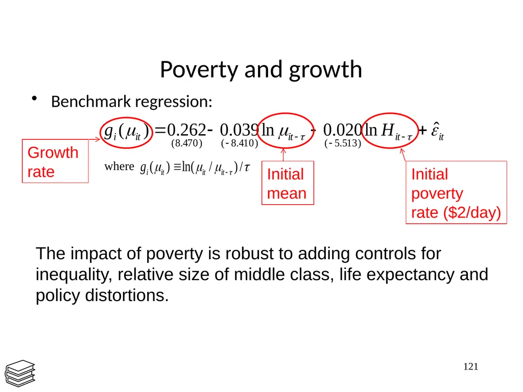
slide121. Poverty and growth Benchmark regression:

where 121 Growth
rate Initial
mean Initial
poverty
rate ($2/day) The impact of poverty is robust to adding controls for inequality, relative size of middle class, life expectancy and policy distortions.<br>
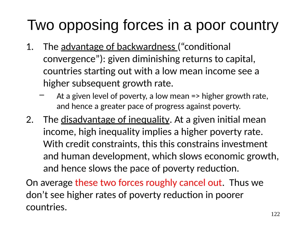
slide122. Two opposing forces in a poor country The advantage of backwardness (“conditional convergence”): given diminishing returns to capital, countries starting out with a low mean income see a higher subsequent growth rate.
At a given level of poverty, a low mean => higher growth rate, and hence a greater pace of progress against poverty.
The disadvantage of inequality. At a given initial mean income, high inequality implies a higher poverty rate. With credit constraints, this this constrains investment and human development, which slows economic growth, and hence slows the pace of poverty reduction.
On average these two forces roughly cancel out. Thus we don’t see higher rates of poverty reduction in poorer countries. 122<br>
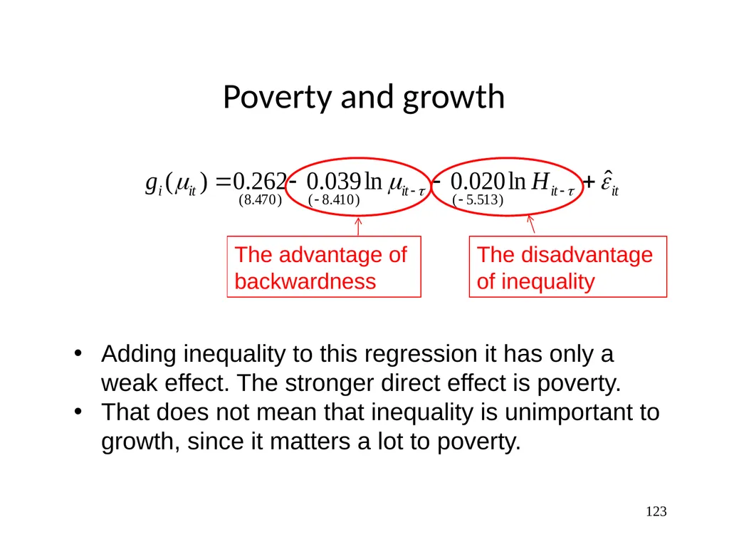
slide123. Poverty and growth 123 The advantage of
backwardness The disadvantage
of inequality Adding inequality to this regression it has only a weak effect. The stronger direct effect is poverty.
That does not mean that inequality is unimportant to growth, since it matters a lot to poverty.<br>
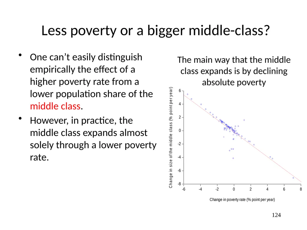
slide124. Less poverty or a bigger middle-class? One can’t easily distinguish empirically the effect of a higher poverty rate from a lower population share of the middle class.
However, in practice, the middle class expands almost solely through a lower poverty rate. 124 The main way that the middle class expands is by declining absolute poverty<br>
slide125. Initial distribution and growth elasticity of poverty reduction Recall: growth elasticity of poverty reduction = proportionate change in the poverty measure divided by rate of growth in the mean consumption or income.
In general, the growth elasticity of poverty reduction will depend on the initial distribution. Intuition: more unequal countries => poor gain less in absolute terms from growth.
High inequality makes growth less inclusive.
But is it inequality or poverty? A high (low) initial poverty rate might also be expected to imply a lower (higher) absolute elasticity.
That is what we see in the data => 125<br>
slide126. Rate of poverty reduction is proportional to the distribution-corrected rate of growth 126<br>
slide127. Poverty makes growth less inclusive The (absolute) growth elasticity of poverty reduction tends to be lower in countries with a higher initial poverty rate.
Poorer countries tend to experience lower proportionate effects on their poverty measures from any given rate of growth.
At an initial poverty rate of 10% (about one standard deviation below the mean) the elasticity is about -3 (using the IVE) while it falls to about -0.7 at a poverty rate of 80% (about one standard deviation above the mean). 127<br>
slide128. In summary High initial poverty puts a break on progress against poverty in two ways:
High poverty makes it harder for the economy to grow, and
High poverty makes growth less pro-poor. 128<br>
slide129. Conclusions 129<br>
slide130. To recap There is an adverse effect on growth of high initial poverty at a given mean.
This is consistent with theoretical models of economic growth incorporating borrowing constraints.
Other explanations include the effects of poor nutrition on learning and productivity.
A high initial incidence of poverty also entails a lower subsequent rate of progress against poverty at a given growth rate. 130<br>
slide131. Implications for development policy? For many poor countries, the growth advantage of starting out with a low mean ("conditional convergence") is lost due to high poverty.
Inequality can be a constraint on growth and (hence) poverty reduction. And high inequality can make growth less poverty reducing.
Not all “inequalities” matter: The key aspect of initial distribution in poor countries is poverty itself, at a given initial mean.
High current inequality is only a handicap if it entails a high incidence of poverty—or (more or less equivalently) a small middle class—at given mean consumption.
Why is poverty such a strong predictor of growth?
Credit market failure story suggests further tests
Child nutrition argument might also be testable. 131<br>
slide132. Policy implications cont., Policies that act directly to reduce poverty can be seen as important elements of longer-term poverty reduction through economic growth.
Two types of policies:
1. Pro-poor redistributive policies (incl. social protection) can have an efficiency role as well their traditional equity role.
2. Policies that make markets work better for the poor, esp. credit, but also land.
In both cases, careful micro evaluation and monitoring will be crucial.
As will flexibility in responding to evidence on what works and what does not in specific contexts. 132<br>
slide133. Aggregate results hide much of importance What aspect of “initial distribution” matters to subsequent growth and poverty reduction?
Inequality or poverty? Poverty may well be the more important factor, but inequality still matters via poverty
Inequality of results or inequality of opportunity? Inequality of opportunity may well be more relevant
Inequality/poverty in what dimension (income vs. non-income factors)? 133<br>