
PLEXOS For Power Systems - Advanced Simulation


Description: PLEXOS For Power Systems - Advanced Simulation Topics Gregory K. Woods Regional Director North America Energy Exemplar, LLC Northwest Power and Conservation Council System Analysis Advisory Committee January 25, 2013 Portland, OR
Related Topics
Download Presentation
"PLEXOS For Power Systems - Advanced Simulation" is the property of its rightful owner. Permission is granted to download and print the materials on this website for personal, non-commercial use only, and to display it on your personal computer provided you do not modify the materials and that you retain all copyright notices contained in the materials. By downloading content from our website, you accept the terms of this agreement.
Presentation Transcript
slide1. PLEXOS For Power Systems -
Advanced Simulation Topics Gregory K. Woods
Regional Director – North America
Energy Exemplar, LLC Northwest Power and Conservation Council
System Analysis Advisory Committee January 25, 2013
Portland, OR<br>
slide2. Confidential | 2 Energy Exemplar, LLC PLEXOS for Power Systems Released in 1999
Continuously Developed to meet Challenges of a Dynamic Environment
A Global Leader in Energy Market Simulation Software With Over 200 Installations in 17 Countries
Offices in Adelaide, Australia; London, UK; California, USA
High Growth Rate in Customers and Installations
Staff Expertise in Operations Research, Electrical Engineering, Economics, Mathematics, Statistics with over 20% Ph.Ds
North American Office:
Consulting
Customer Support
Training
Software Sales
North American Datasets/WECC Term 01/25/13<br>
slide3. PLEXOS For Power Systems
Renewable Portfolio Expansion
OpenPlexos API
Integrated Stochastics
Stochastic Optimization
Multi-Stage Optimization
Stochastic Unit Commitment
Optimal Power Flow Issues
High Performance Computing (HPC) 3 Advanced Simulation Topics Agenda 01/25/13<br>
slide4. Power Market Simulation, Price Forecasting and Analysis
Operational Planning, Unit Commitment and Optimisation of Generation and Transmission
Trading and Strategic Decision Support
Integrated Resource Plan including Generation and Transmission Expansion and Investment Analysis
Renewable Integration Analysis and Intermittent Supply
Co-optimisation of Ancillary Services, Energy Dispatch and Emissions
Transmission Analysis and Congestion Management
Portfolio Optimisation and Valuation
Risk Management and Stochastic Optimisation 4 PLEXOS for Power Systems 01/25/13<br>
slide5. 5 PLEXOS Algorithms Mathematical Optimization
Utilizes world-class commercial solvers
Integrates Mixed Integer, Dynamic and Linear Programming Techniques to provide fast, accurate results
Simultaneous Co-optimization:
Capacity Expansion, Reliability, Security Constraints, Unit Commitment and Economic dispatch, revenue adequacy and uplift
Thermal, Hydro, Energy, Reserve, Fuel, and Emissions Markets
Integrated Stochastic Optimization
Solves the Perfect Foresight Problem using a multi-stage optimizer that includes sample reduction for fast accurate results
User-defined constraints and decision variables
Powerful formulation replaces the need for expensive custom programming
Both physical (primal) and financial (dual) results reported
Shadow Pricing report the real operating costs in constrained environments
OpenPlexos allows customization and automation of PLEXOS through a standardized Application Programming Interface (API) 01/25/13 Confidential & Proprietary Information<br>
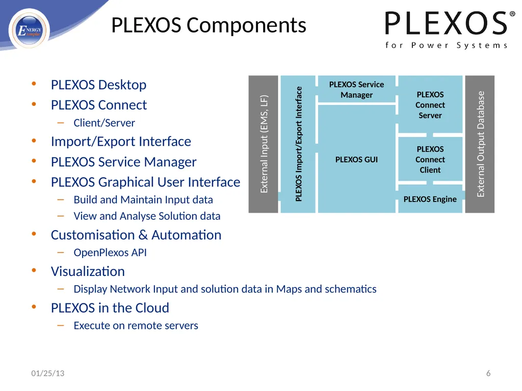
slide6. PLEXOS Desktop
PLEXOS Connect
Client/Server
Import/Export Interface
PLEXOS Service Manager
PLEXOS Graphical User Interface
Build and Maintain Input data
View and Analyse Solution data
Customisation & Automation
OpenPlexos API
Visualization
Display Network Input and solution data in Maps and schematics
PLEXOS in the Cloud
Execute on remote servers 6 PLEXOS Components 01/25/13<br>
slide7. Over 150 technical and economic generation characteristics:
Deterministic and stochastic unit commitment
Random and scheduled outages - optimized maintenance
Temperature-dependent operating characteristics
Detailed ramping and start/stop profiles
Multiple fuel optimisation with complex fuel transitions and operational modes
Compartmentalised combined cycle modelling featuring non-convex heat rates
Unit Dependencies 7 Simulation Features - Conventional Generation 01/25/13<br>
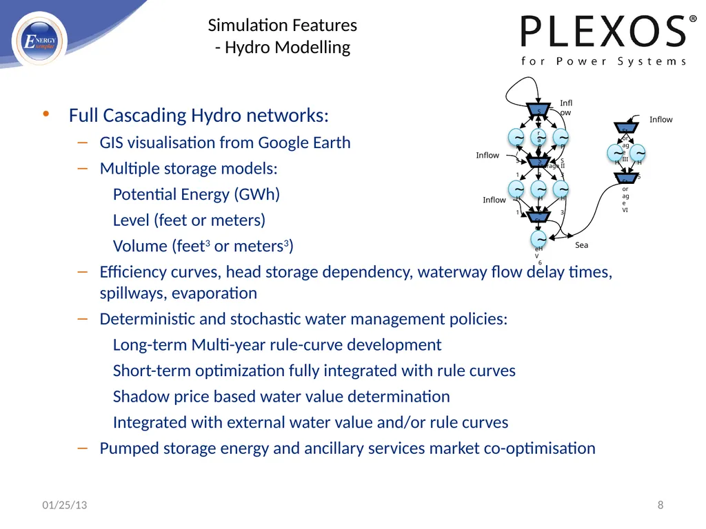
slide8. Full Cascading Hydro networks:
GIS visualisation from Google Earth
Multiple storage models:
Potential Energy (GWh)
Level (feet or meters)
Volume (feet3 or meters3)
Efficiency curves, head storage dependency, waterway flow delay times, spillways, evaporation
Deterministic and stochastic water management policies:
Long-term Multi-year rule-curve development
Short-term optimization fully integrated with rule curves
Shadow price based water value determination
Integrated with external water value and/or rule curves
Pumped storage energy and ancillary services market co-optimisation 8 Simulation Features - Hydro Modelling 01/25/13<br>
slide9. Ancillary services
Co-optimised with generation dispatch and unit commitment and more features such as:
Multiple reserve classes including spinning up and down, regulation up and down, and replacement services
Detailed treatment of start-up and shutdown combined with ramping and reserve interaction over user-selectable intervals down to 1-minute
Emissions
Co-optimized generation dispatch for emission limits, emission prices and/or allowances
Emissions production on start/up, fuel use, and generation
Multiple removal technologies including limestone, ammonia, activated carbon
Flexible Emission constraints including plant, region, zone on any period including multi-year constraints
Multiple Air District rules
Demand Side Management
Supports multiple technologies such as distributed generation, demand response bidding, and curtail-able load
Value DSM programs cost to the system, risk value, capacity value, and valuation 9 Simulation Features - Additional 01/25/13<br>
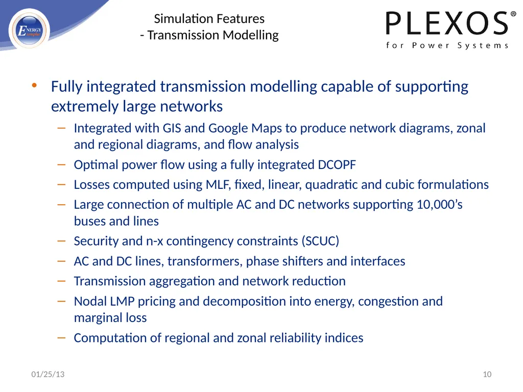
slide10. Fully integrated transmission modelling capable of supporting extremely large networks
Integrated with GIS and Google Maps to produce network diagrams, zonal and regional diagrams, and flow analysis
Optimal power flow using a fully integrated DCOPF
Losses computed using MLF, fixed, linear, quadratic and cubic formulations
Large connection of multiple AC and DC networks supporting 10,000’s buses and lines
Security and n-x contingency constraints (SCUC)
AC and DC lines, transformers, phase shifters and interfaces
Transmission aggregation and network reduction
Nodal LMP pricing and decomposition into energy, congestion and marginal loss
Computation of regional and zonal reliability indices 10 Simulation Features - Transmission Modelling 01/25/13<br>
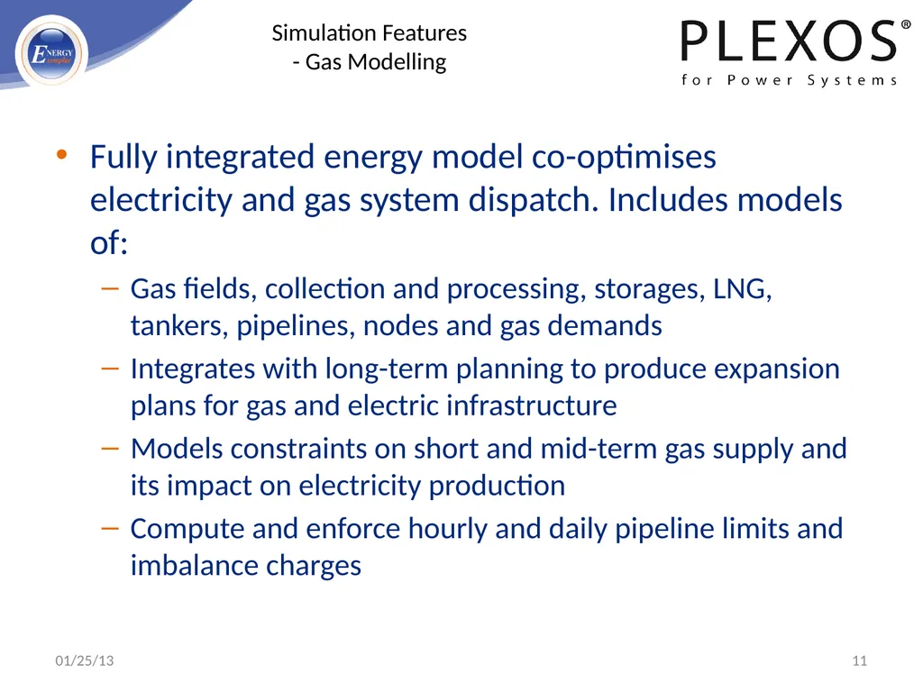
slide11. Fully integrated energy model co-optimises electricity and gas system dispatch. Includes models of:
Gas fields, collection and processing, storages, LNG, tankers, pipelines, nodes and gas demands
Integrates with long-term planning to produce expansion plans for gas and electric infrastructure
Models constraints on short and mid-term gas supply and its impact on electricity production
Compute and enforce hourly and daily pipeline limits and imbalance charges 11 Simulation Features - Gas Modelling 01/25/13<br>
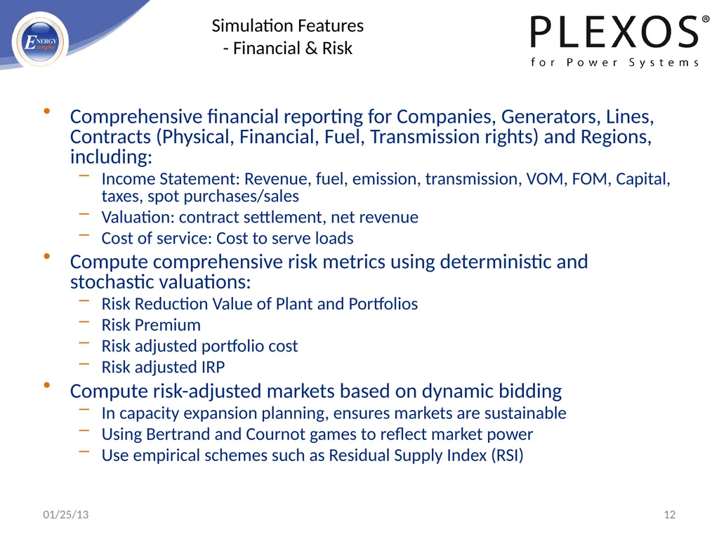
slide12. Comprehensive financial reporting for Companies, Generators, Lines, Contracts (Physical, Financial, Fuel, Transmission rights) and Regions, including:
Income Statement: Revenue, fuel, emission, transmission, VOM, FOM, Capital, taxes, spot purchases/sales
Valuation: contract settlement, net revenue
Cost of service: Cost to serve loads
Compute comprehensive risk metrics using deterministic and stochastic valuations:
Risk Reduction Value of Plant and Portfolios
Risk Premium
Risk adjusted portfolio cost
Risk adjusted IRP
Compute risk-adjusted markets based on dynamic bidding
In capacity expansion planning, ensures markets are sustainable
Using Bertrand and Cournot games to reflect market power
Use empirical schemes such as Residual Supply Index (RSI) 12 Simulation Features - Financial & Risk 01/25/13<br>
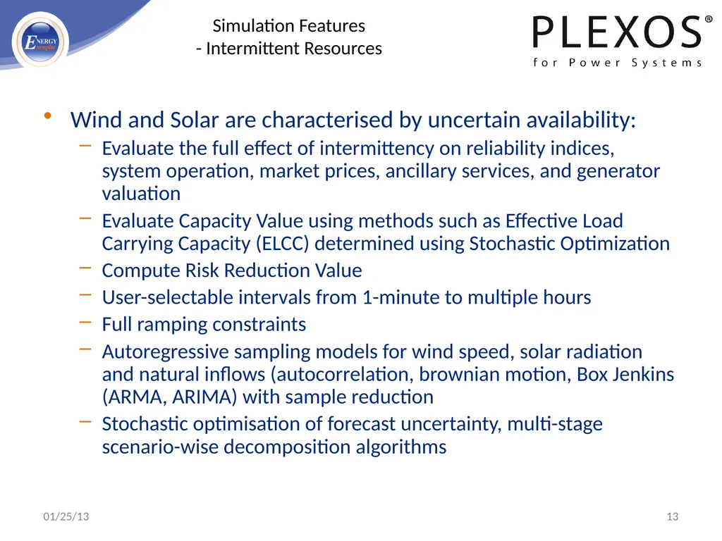
slide13. Wind and Solar are characterised by uncertain availability:
Evaluate the full effect of intermittency on reliability indices, system operation, market prices, ancillary services, and generator valuation
Evaluate Capacity Value using methods such as Effective Load Carrying Capacity (ELCC) determined using Stochastic Optimization
Compute Risk Reduction Value
User-selectable intervals from 1-minute to multiple hours
Full ramping constraints
Autoregressive sampling models for wind speed, solar radiation and natural inflows (autocorrelation, brownian motion, Box Jenkins (ARMA, ARIMA) with sample reduction
Stochastic optimisation of forecast uncertainty, multi-stage scenario-wise decomposition algorithms 13 Simulation Features - Intermittent Resources 01/25/13<br>
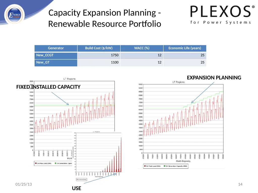
slide14. Capacity Expansion Planning - Renewable Resource Portfolio FIXED INSTALLED CAPACITY USE EXPANSION PLANNING 14 01/25/13<br>
slide15. Transmission Expansion General Description:
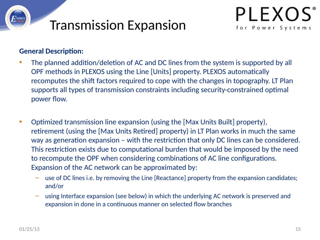
The planned addition/deletion of AC and DC lines from the system is supported by all OPF methods in PLEXOS using the Line [Units] property. PLEXOS automatically recomputes the shift factors required to cope with the changes in topography. LT Plan supports all types of transmission constraints including security-constrained optimal power flow.
Optimized transmission line expansion (using the [Max Units Built] property), retirement (using the [Max Units Retired] property) in LT Plan works in much the same way as generation expansion – with the restriction that only DC lines can be considered. This restriction exists due to computational burden that would be imposed by the need to recompute the OPF when considering combinations of AC line configurations. Expansion of the AC network can be approximated by:
use of DC lines i.e. by removing the Line [Reactance] property from the expansion candidates; and/or
using Interface expansion (see below) in which the underlying AC network is preserved and expansion in done in a continuous manner on selected flow branches 15 01/25/13<br>
slide16. What is OpenPlexos:
API accessible through Visual Studio.NET
API accessible through any CSI language
http://en.wikipedia.org/wiki/List_of_CLI_languages
Uses:
Custom Input
Integration with Other Applications
Control Execution: Triggers with SCADA, etc.
Control Execution: Add additional Optimization Logic
Control Execution: Custom Risk Logic
Custom Reporting (Additional Properties, New Formats)
Write to SQL Server or other DBMS 16 Introduction to OpenPlexos 01/25/13<br>
slide17. COM - Microsoft Component Object Model technology.
A Microsoft designed framework for program interoperability. Many programming environments allow COM compliant calls, including VBA in Office.
PLEXOS COM provides functions to change input, execute models and projects, and query solutions
.NET - Microsoft .NET Framework.
A programming framework for application development. Resulting programs are easier to produce and maintain, more consistent and less prone to bugs. They require .NET to run
PLEXOS uses .NET
API - Application Programming Interface.
A series of embedded system calls and a defined object model that allows programmers to access and modify applications. A good example is the Excel object model in VBA which allows programmers to modify the way Excel function by embedding code.
PLEXOS has an API accessible through .NET compliant programming environments like Visual Studio
PLEXOS API allows for customization and process control
AMMO - ActiveX Mathematical Modeling Objects
Proprietary Optimization layer in PLEXOS.
Interface AMMO to customize simulations using VS.NET 17 Application Programming Interface Many Microsoft and Other Windows-based environments allow connections to COM compliant applications including PLEXOS.
PLEXOS can be automated from many environments, including Office and SQLServer 01/25/13<br>
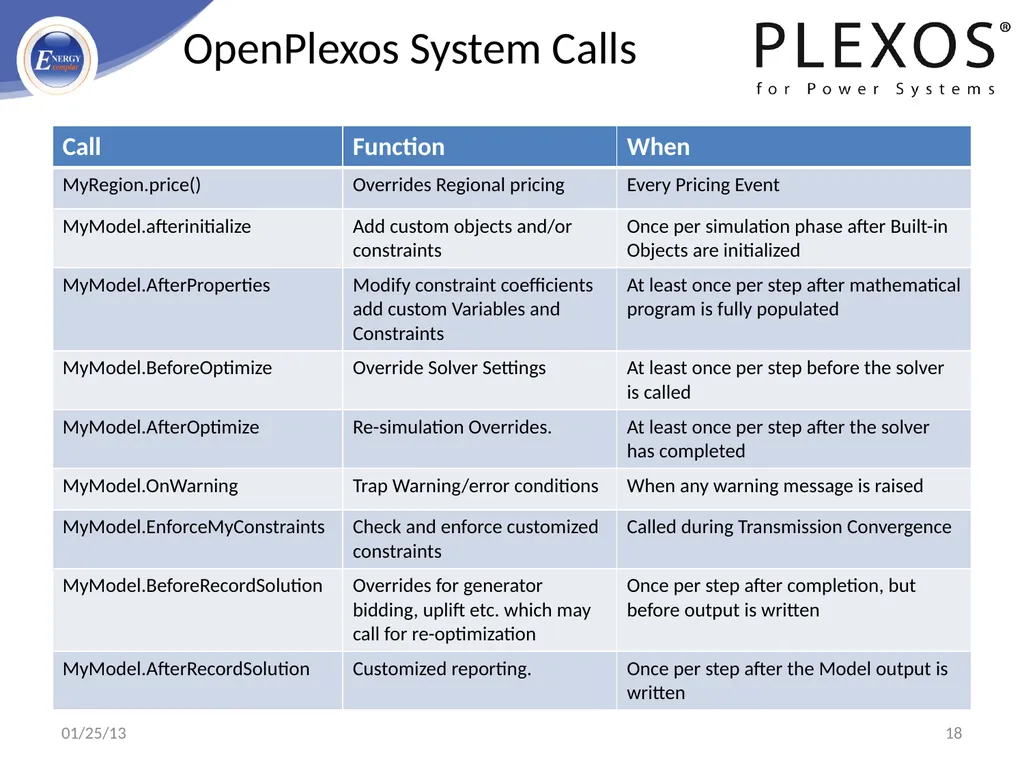
slide18. 18 OpenPlexos System Calls 01/25/13<br>
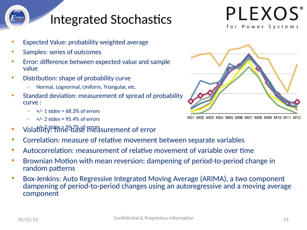
slide19. 19 Integrated Stochastics Expected Value: probability weighted average
Samples: series of outcomes
Error: difference between expected value and sample value
Distribution: shape of probability curve
Normal, Lognormal, Uniform, Triangular, etc.
Standard deviation: measurement of spread of probability curve :
+/- 1 stdev = 68.3% of errors
+/- 2 stdev = 95.4% of errors
+/- 3 stdev = 99.7% of errors 01/25/13 Confidential & Proprietary Information Volatility: time-base measurement of error
Correlation: measure of relative movement between separate variables
Autocorrelation: measurement of relative movement of variable over time
Brownian Motion with mean reversion: dampening of period-to-period change in random patterns
Box-Jenkins: Auto Regressive Integrated Moving Average (ARIMA), a two component dampening of period-to-period changes using an autoregressive and a moving average component<br>
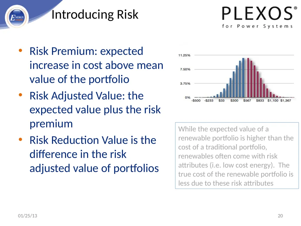
slide20. Risk Premium: expected increase in cost above mean value of the portfolio
Risk Adjusted Value: the expected value plus the risk premium
Risk Reduction Value is the difference in the risk adjusted value of portfolios 01/25/13 20 Introducing Risk While the expected value of a renewable portfolio is higher than the cost of a traditional portfolio, renewables often come with risk attributes (i.e. low cost energy). The true cost of the renewable portfolio is less due to these risk attributes<br>
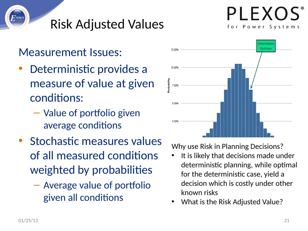
slide21. Measurement Issues:
Deterministic provides a measure of value at given conditions:
Value of portfolio given average conditions
Stochastic measures values of all measured conditions weighted by probabilities
Average value of portfolio given all conditions 01/25/13 21 Risk Adjusted Values Why use Risk in Planning Decisions?
It is likely that decisions made under deterministic planning, while optimal for the deterministic case, yield a decision which is costly under other known risks
What is the Risk Adjusted Value?<br>
slide22. The Perfect Foresight Problem:
Stochastic Run is simply a deterministic (predictable) run using randomly drawn data
Optimization therefore assumes that you know the outcome, i.e. have perfect foresight
What if you need to make a decision (UC, Hydro schedule, Build/retire), based on an unknown future?
Stochastic Optimization makes the decision, then evaluates then runs stochastic optimizations, allowing the best decision to be determined 01/25/13 22 Short-Comings of Deterministic Simulation<br>
slide23. Fix perfect foresight issue
Monte Carlo simulation can tell us what the optimal decision is for each of a number of possible outcomes assuming perfect foresight for each scenario independently;
It cannot answer the question: what decision should I make now given the uncertainty in the inputs?
Stochastic Programming
The goal of SO is to find some policy that is feasible for all (or almost all) of the possible data instances and maximize the expectation of some function of the decisions and the random variables
Scenario-wise decomposition
The set of all outcomes is represented as “scenarios”, the set of scenarios can be reduced by grouping like scenarios together. The reduced sample size can be run more efficiently 23 Stochastic Optimization (SO) 01/25/13 Confidential & Proprietary Information<br>
slide24. SO Theory The most widely applied and studied stochastic programming models are two-stage linear programs
Here the decision maker takes some action in the first stage, after which a random event occurs affecting the outcome of the first-stage decision
A recourse decision can then be made in the second stage that compensates for any bad effects that might have been experienced as a result of the first-stage decision
The optimal policy from such a model is a single first-stage policy and a collection of recourse decisions (a decision rule) defining which second-stage action should be taken in response to each random outcome 24 01/25/13<br>
slide25. SO Theory, Continued Where the first (or second) stage decisions must take integer values we have a stochastic integer programming (SIP) problem
SIP problems are difficult to solve in general
Assuming integer first-stage decisions (e.g. “how many generators of type x to build” or “when do a turn on/off this power plant”) we want to find a solution that minimises the total cost of the first and second stage decisions
A number of solution approaches have been suggested in the literature
PLEXOS uses scenario-wise decomposition ... 25 01/25/13<br>
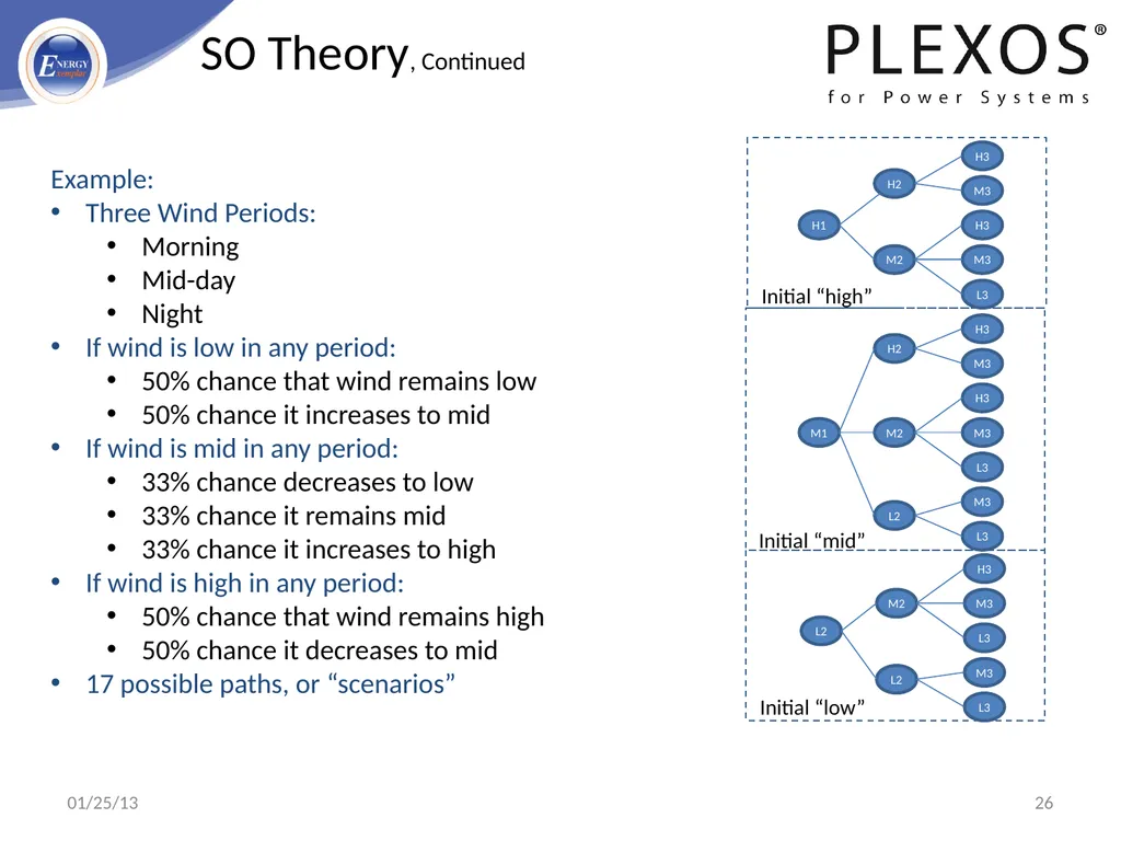
slide26. SO Theory, Continued Example:
Three Wind Periods:
Morning
Mid-day
Night
If wind is low in any period:
50% chance that wind remains low
50% chance it increases to mid
If wind is mid in any period:
33% chance decreases to low
33% chance it remains mid
33% chance it increases to high
If wind is high in any period:
50% chance that wind remains high
50% chance it decreases to mid
17 possible paths, or “scenarios” 26 01/25/13<br>
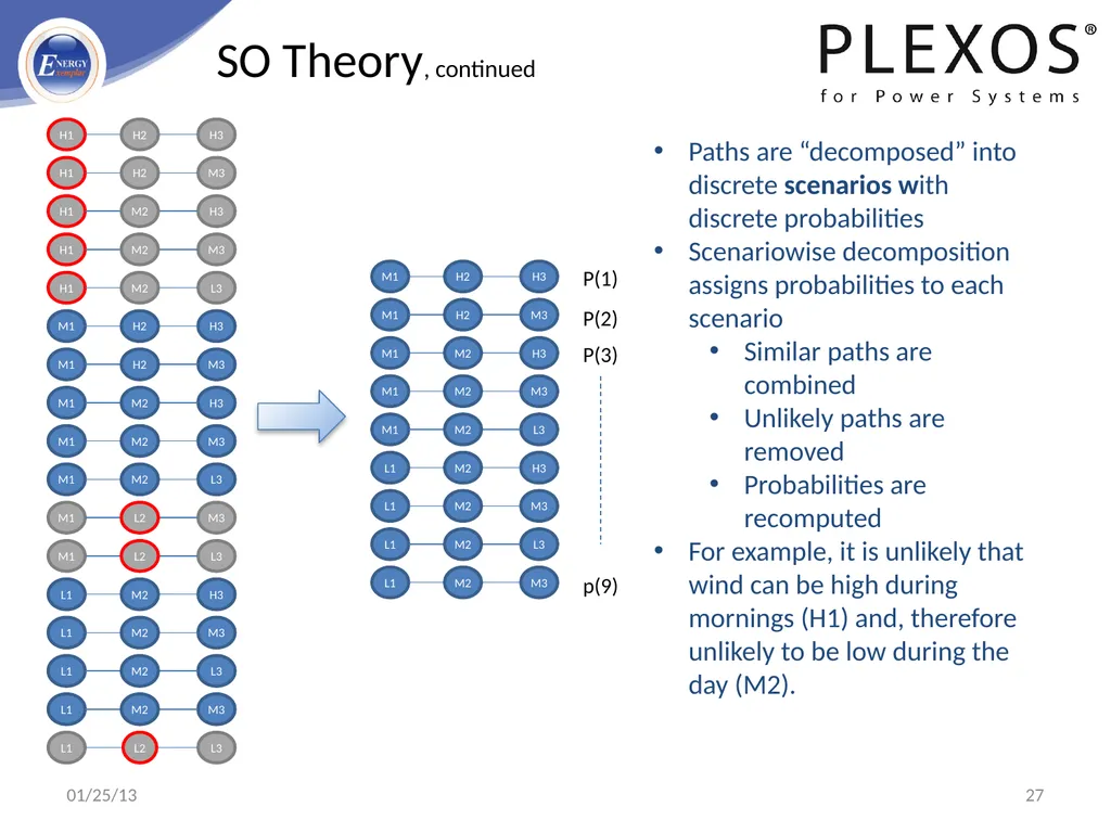
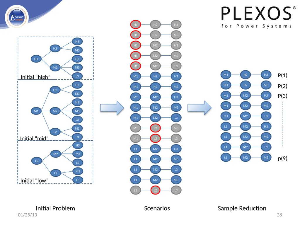
slide27. SO Theory, continued Paths are “decomposed” into discrete scenarios with discrete probabilities
Scenariowise decomposition assigns probabilities to each scenario
Similar paths are combined
Unlikely paths are removed
Probabilities are recomputed
For example, it is unlikely that wind can be high during mornings (H1) and, therefore unlikely to be low during the day (M2). 27 01/25/13<br>
slide28. 28 Initial Problem Scenarios Sample Reduction 01/25/13<br>
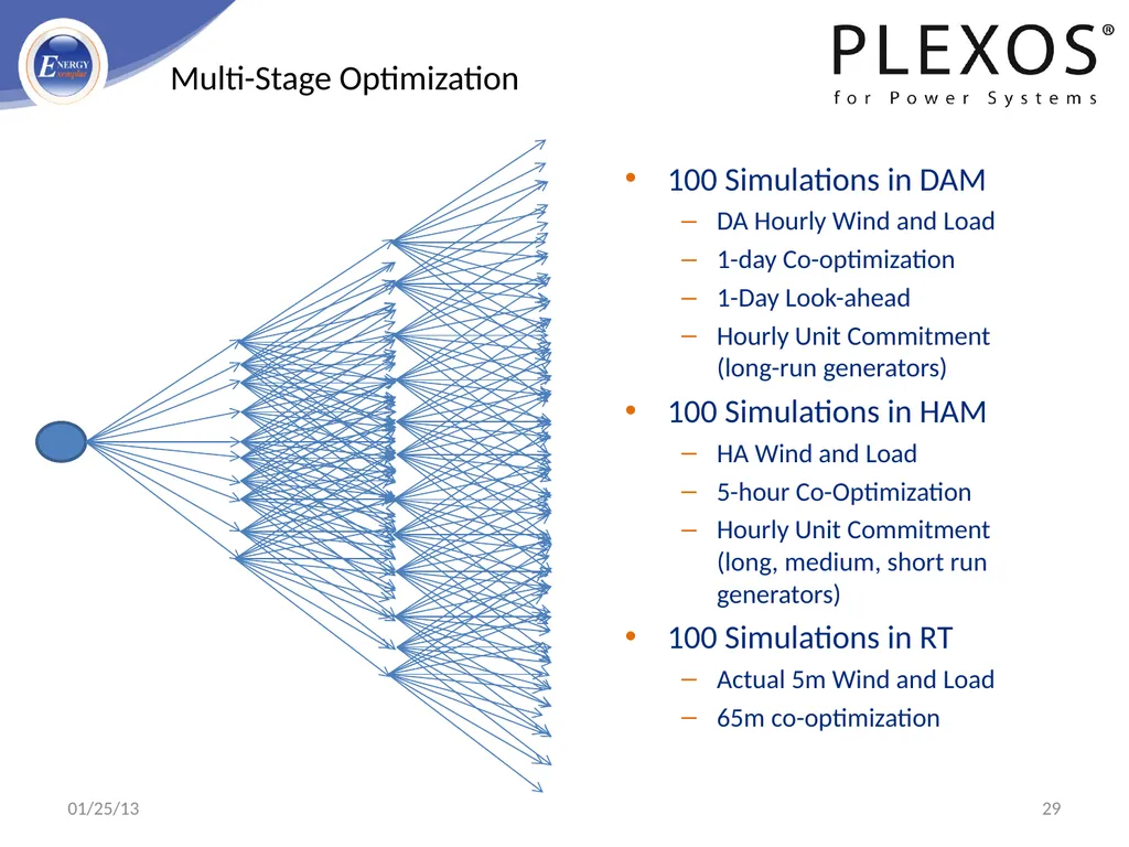
slide29. 01/25/13 29 Multi-Stage Optimization 100 Simulations in DAM
DA Hourly Wind and Load
1-day Co-optimization
1-Day Look-ahead
Hourly Unit Commitment (long-run generators)
100 Simulations in HAM
HA Wind and Load
5-hour Co-Optimization
Hourly Unit Commitment (long, medium, short run generators)
100 Simulations in RT
Actual 5m Wind and Load
65m co-optimization<br>
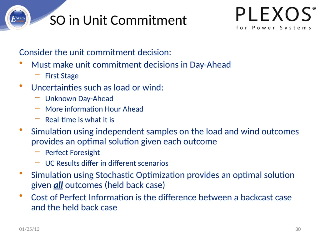
slide30. SO in Unit Commitment Consider the unit commitment decision:
Must make unit commitment decisions in Day-Ahead
First Stage
Uncertainties such as load or wind:
Unknown Day-Ahead
More information Hour Ahead
Real-time is what it is
Simulation using independent samples on the load and wind outcomes provides an optimal solution given each outcome
Perfect Foresight
UC Results differ in different scenarios
Simulation using Stochastic Optimization provides an optimal solution given all outcomes (held back case)
Cost of Perfect Information is the difference between a backcast case and the held back case 30 01/25/13<br>
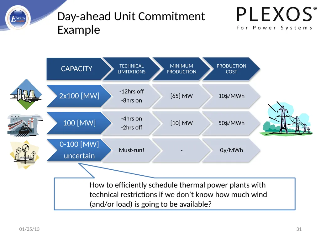
slide31. Day-ahead Unit Commitment Example How to efficiently schedule thermal power plants with technical restrictions if we don’t know how much wind (and/or load) is going to be available? 31 01/25/13<br>
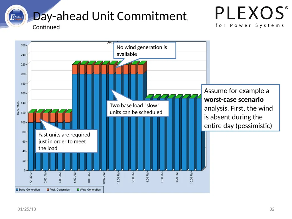
slide32. Day-ahead Unit Commitment, Continued Assume for example a worst-case scenario analysis. First, the wind is absent during the entire day (pessimistic) Two base load “slow” units can be scheduled Fast units are required just in order to meet the load No wind generation is available 32 01/25/13<br>
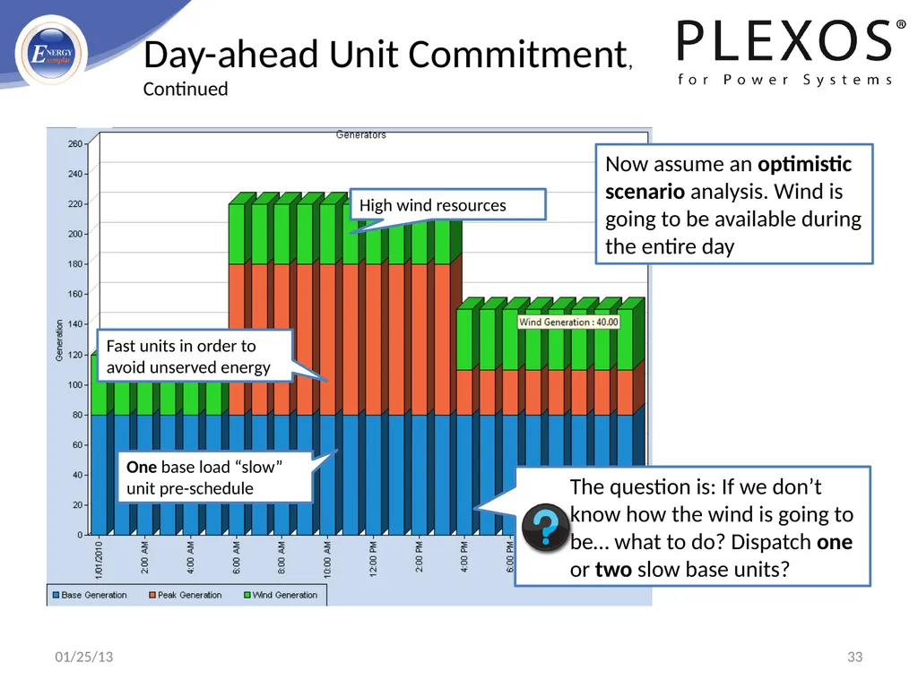
slide33. Day-ahead Unit Commitment, Continued Now assume an optimistic scenario analysis. Wind is going to be available during the entire day One base load “slow” unit pre-schedule Fast units in order to avoid unserved energy High wind resources The question is: If we don’t know how the wind is going to be… what to do? Dispatch one or two slow base units? 33 01/25/13<br>
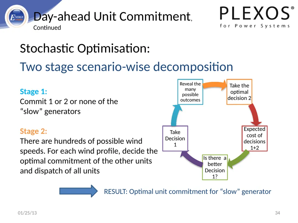
slide34. Day-ahead Unit Commitment, Continued Stochastic Optimisation:
Two stage scenario-wise decomposition Stage 1:
Commit 1 or 2 or none of the
“slow” generators
Stage 2:
There are hundreds of possible wind speeds. For each wind profile, decide the
optimal commitment of the other units and dispatch of all units 34 RESULT: Optimal unit commitment for “slow” generator 01/25/13<br>
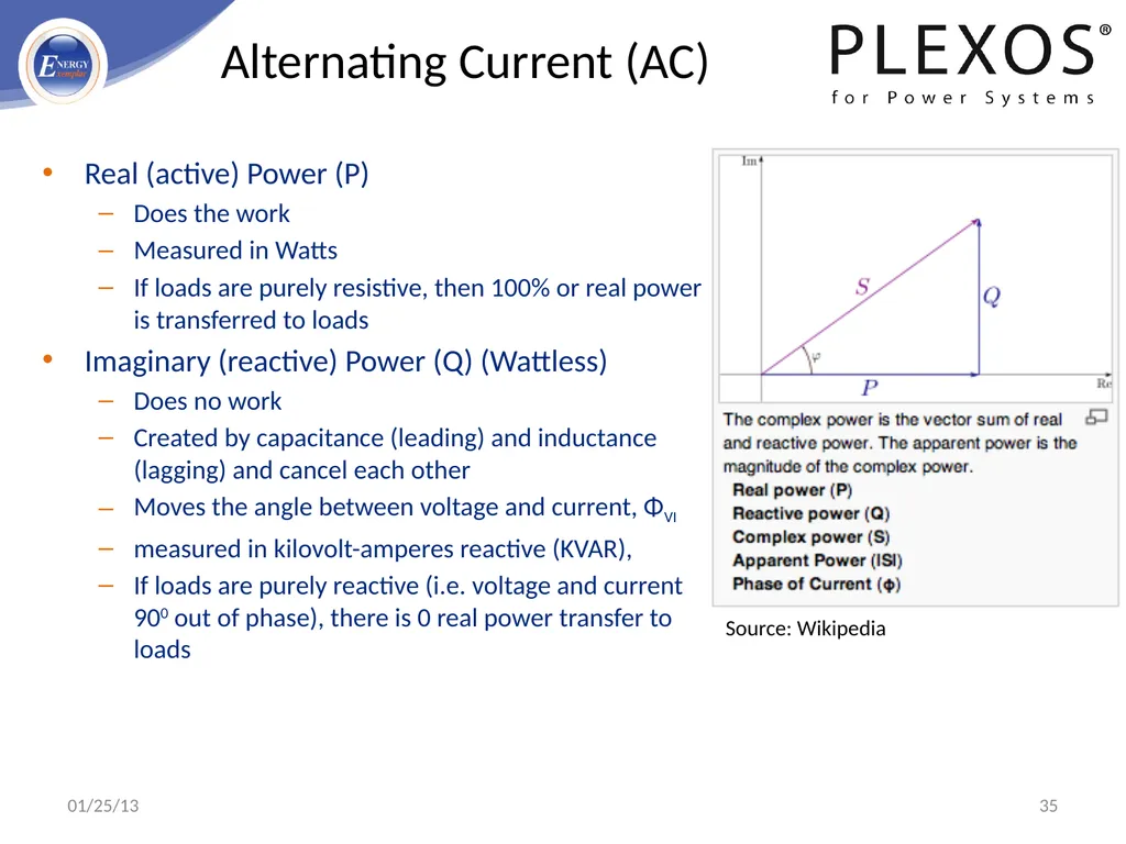
slide35. Real (active) Power (P)
Does the work
Measured in Watts
If loads are purely resistive, then 100% or real power is transferred to loads
Imaginary (reactive) Power (Q) (Wattless)
Does no work
Created by capacitance (leading) and inductance (lagging) and cancel each other
Moves the angle between voltage and current, ΦVI
measured in kilovolt-amperes reactive (KVAR),
If loads are purely reactive (i.e. voltage and current 900 out of phase), there is 0 real power transfer to loads 35 Alternating Current (AC) Source: Wikipedia 01/25/13<br>
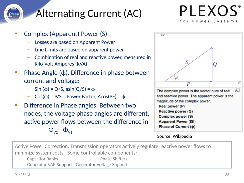
slide36. Complex (Apparent) Power (S)
Losses are based on Apparent Power
Line Limits are based on apparent power
Combination of real and reactive power, measured in Kilo-Volt Amperes (KVA).
Phase Angle (ϕ). Difference in phase between current and voltage:
Sin (ϕ) = Q/S, asin(Q/S) = ϕ
Cos(ϕ) = P/S = Power Factor, Acos(PF) = ϕ
Difference in Phase angles: Between two nodes, the voltage phase angles are different, active power flows between the difference in ΦV2 - ΦV1 36 Alternating Current (AC) Source: Wikipedia Active Power Correction: Transmission operators actively regulate reactive power flows to minimize system costs. Some controllable components:
Capacitor Banks Phase Shifters
Generator VAR Support Generator Voltage Support 01/25/13<br>
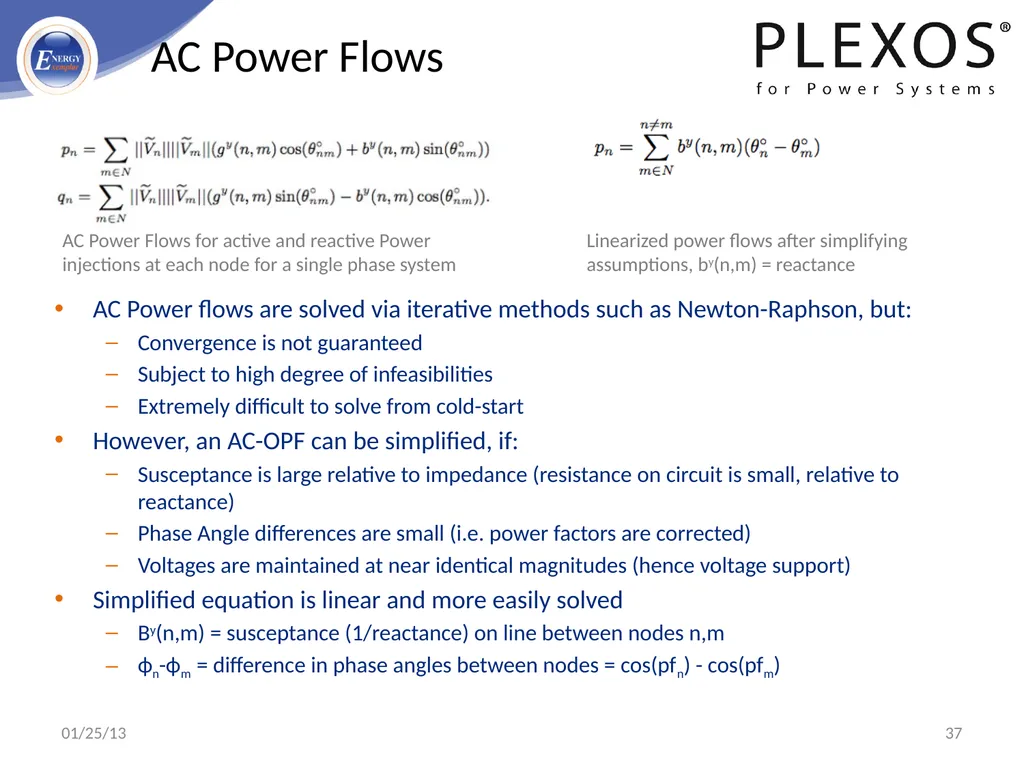
slide37. 37 AC Power Flows AC Power flows are solved via iterative methods such as Newton-Raphson, but:
Convergence is not guaranteed
Subject to high degree of infeasibilities
Extremely difficult to solve from cold-start
However, an AC-OPF can be simplified, if:
Susceptance is large relative to impedance (resistance on circuit is small, relative to reactance)
Phase Angle differences are small (i.e. power factors are corrected)
Voltages are maintained at near identical magnitudes (hence voltage support)
Simplified equation is linear and more easily solved
By(n,m) = susceptance (1/reactance) on line between nodes n,m
ϕn-ϕm = difference in phase angles between nodes = cos(pfn) - cos(pfm) AC Power Flows for active and reactive Power injections at each node for a single phase system Linearized power flows after simplifying assumptions, by(n,m) = reactance 01/25/13<br>
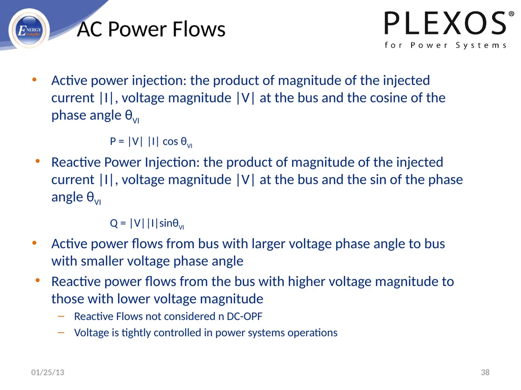
slide38. 38 AC Power Flows Active power injection: the product of magnitude of the injected current |I|, voltage magnitude |V| at the bus and the cosine of the phase angle θVI
P = |V| |I| cos θVI
Reactive Power Injection: the product of magnitude of the injected current |I|, voltage magnitude |V| at the bus and the sin of the phase angle θVI
Q = |V||I|sinθVI
Active power flows from bus with larger voltage phase angle to bus with smaller voltage phase angle
Reactive power flows from the bus with higher voltage magnitude to those with lower voltage magnitude
Reactive Flows not considered n DC-OPF
Voltage is tightly controlled in power systems operations 01/25/13<br>
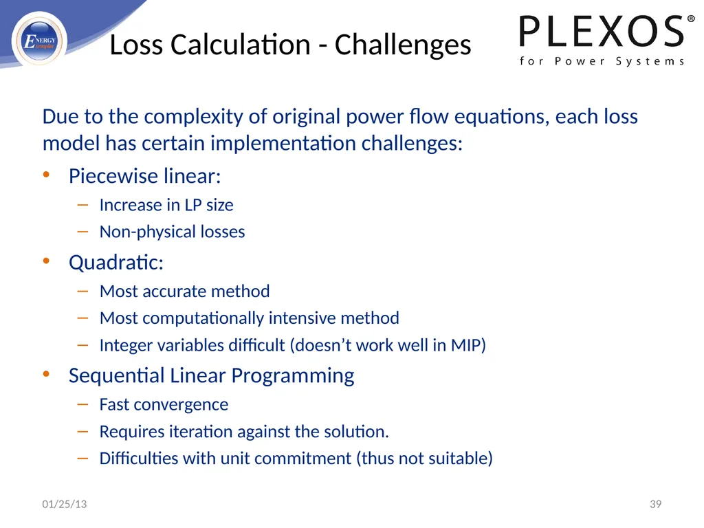
slide39. Loss Calculation - Challenges Due to the complexity of original power flow equations, each loss model has certain implementation challenges:
Piecewise linear:
Increase in LP size
Non-physical losses
Quadratic:
Most accurate method
Most computationally intensive method
Integer variables difficult (doesn’t work well in MIP)
Sequential Linear Programming
Fast convergence
Requires iteration against the solution.
Difficulties with unit commitment (thus not suitable) 39 01/25/13<br>
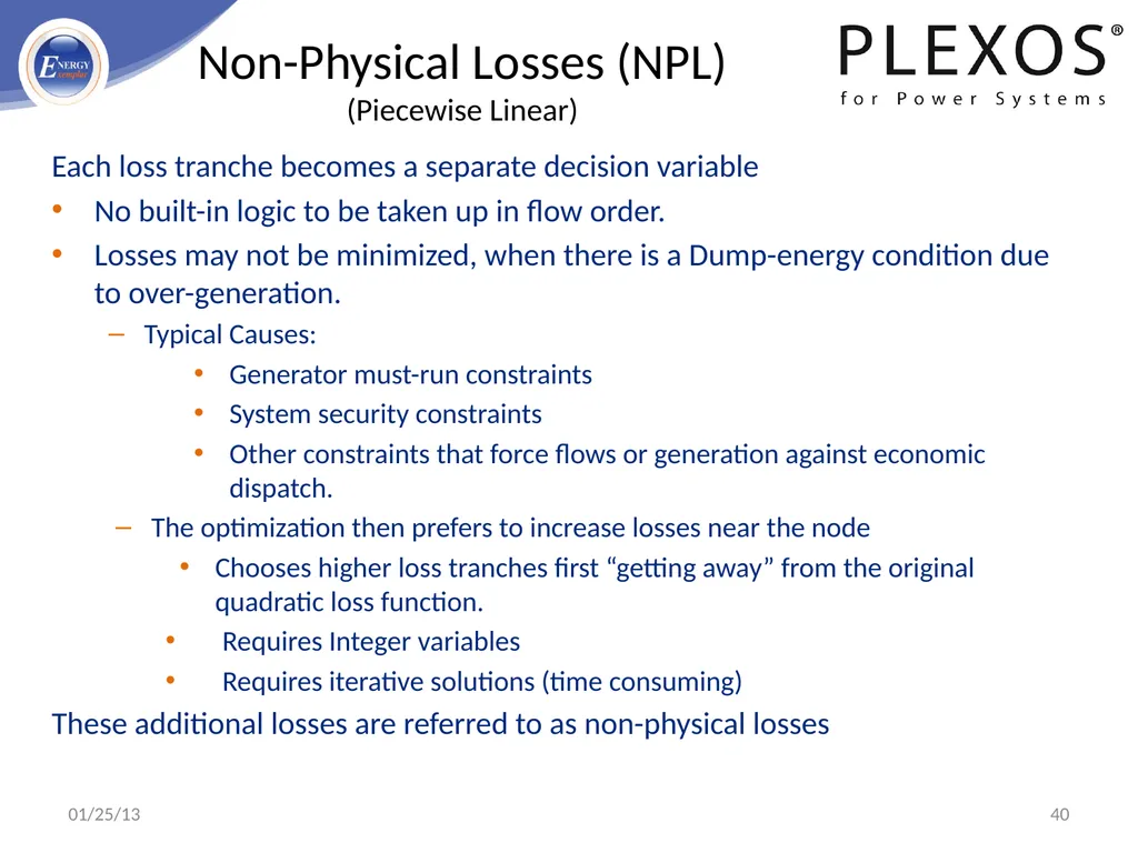
slide40. Non-Physical Losses (NPL) (Piecewise Linear) Each loss tranche becomes a separate decision variable
No built-in logic to be taken up in flow order.
Losses may not be minimized, when there is a Dump-energy condition due to over-generation.
Typical Causes:
Generator must-run constraints
System security constraints
Other constraints that force flows or generation against economic dispatch.
The optimization then prefers to increase losses near the node
Chooses higher loss tranches first “getting away” from the original quadratic loss function.
Requires Integer variables
Requires iterative solutions (time consuming)
These additional losses are referred to as non-physical losses 40 01/25/13<br>
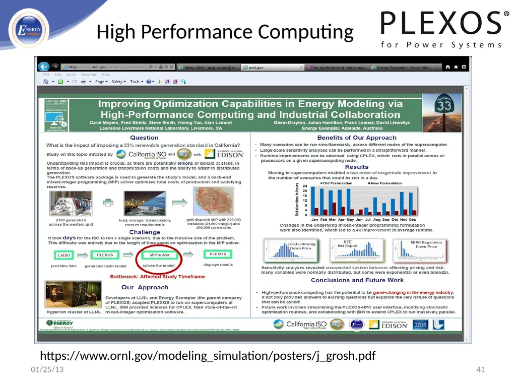
slide41. 01/25/13 41 High Performance Computing https://www.ornl.gov/modeling_simulation/posters/j_grosh.pdf<br>
slide42. Questions
Gregory K. Woods
Regional Director – North America
Energy Exemplar, LLC 01/25/13 42 Energy Exemplar Ltd Building 3, Chiswick Park 566 Chiswick High Road Chiswick London W4 5YA, UK Tel: +44 208 899 6500 www.energyexemplar.com Energy Exemplar Pty Ltd
Suite 3, 154-160 Prospect Road
Prospect
SA 4082 Australia
Tel: +61 8 8342 9616 Energy Exemplar LLC 3013 Douglas Blvd, Ste. 120 Roseville, CA 95661 USA
Tel: +1 916 722 1484<br>
Regional Director – North America
Energy Exemplar, LLC Northwest Power and Conservation Council
System Analysis Advisory Committee January 25, 2013
Portland, OR<br>
slide2. Confidential | 2 Energy Exemplar, LLC PLEXOS for Power Systems Released in 1999
Continuously Developed to meet Challenges of a Dynamic Environment
A Global Leader in Energy Market Simulation Software With Over 200 Installations in 17 Countries
Offices in Adelaide, Australia; London, UK; California, USA
High Growth Rate in Customers and Installations
Staff Expertise in Operations Research, Electrical Engineering, Economics, Mathematics, Statistics with over 20% Ph.Ds
North American Office:
Consulting
Customer Support
Training
Software Sales
North American Datasets/WECC Term 01/25/13<br>
slide3. PLEXOS For Power Systems
Renewable Portfolio Expansion
OpenPlexos API
Integrated Stochastics
Stochastic Optimization
Multi-Stage Optimization
Stochastic Unit Commitment
Optimal Power Flow Issues
High Performance Computing (HPC) 3 Advanced Simulation Topics Agenda 01/25/13<br>
slide4. Power Market Simulation, Price Forecasting and Analysis
Operational Planning, Unit Commitment and Optimisation of Generation and Transmission
Trading and Strategic Decision Support
Integrated Resource Plan including Generation and Transmission Expansion and Investment Analysis
Renewable Integration Analysis and Intermittent Supply
Co-optimisation of Ancillary Services, Energy Dispatch and Emissions
Transmission Analysis and Congestion Management
Portfolio Optimisation and Valuation
Risk Management and Stochastic Optimisation 4 PLEXOS for Power Systems 01/25/13<br>
slide5. 5 PLEXOS Algorithms Mathematical Optimization
Utilizes world-class commercial solvers
Integrates Mixed Integer, Dynamic and Linear Programming Techniques to provide fast, accurate results
Simultaneous Co-optimization:
Capacity Expansion, Reliability, Security Constraints, Unit Commitment and Economic dispatch, revenue adequacy and uplift
Thermal, Hydro, Energy, Reserve, Fuel, and Emissions Markets
Integrated Stochastic Optimization
Solves the Perfect Foresight Problem using a multi-stage optimizer that includes sample reduction for fast accurate results
User-defined constraints and decision variables
Powerful formulation replaces the need for expensive custom programming
Both physical (primal) and financial (dual) results reported
Shadow Pricing report the real operating costs in constrained environments
OpenPlexos allows customization and automation of PLEXOS through a standardized Application Programming Interface (API) 01/25/13 Confidential & Proprietary Information<br>
slide6. PLEXOS Desktop
PLEXOS Connect
Client/Server
Import/Export Interface
PLEXOS Service Manager
PLEXOS Graphical User Interface
Build and Maintain Input data
View and Analyse Solution data
Customisation & Automation
OpenPlexos API
Visualization
Display Network Input and solution data in Maps and schematics
PLEXOS in the Cloud
Execute on remote servers 6 PLEXOS Components 01/25/13<br>
slide7. Over 150 technical and economic generation characteristics:
Deterministic and stochastic unit commitment
Random and scheduled outages - optimized maintenance
Temperature-dependent operating characteristics
Detailed ramping and start/stop profiles
Multiple fuel optimisation with complex fuel transitions and operational modes
Compartmentalised combined cycle modelling featuring non-convex heat rates
Unit Dependencies 7 Simulation Features - Conventional Generation 01/25/13<br>
slide8. Full Cascading Hydro networks:
GIS visualisation from Google Earth
Multiple storage models:
Potential Energy (GWh)
Level (feet or meters)
Volume (feet3 or meters3)
Efficiency curves, head storage dependency, waterway flow delay times, spillways, evaporation
Deterministic and stochastic water management policies:
Long-term Multi-year rule-curve development
Short-term optimization fully integrated with rule curves
Shadow price based water value determination
Integrated with external water value and/or rule curves
Pumped storage energy and ancillary services market co-optimisation 8 Simulation Features - Hydro Modelling 01/25/13<br>
slide9. Ancillary services
Co-optimised with generation dispatch and unit commitment and more features such as:
Multiple reserve classes including spinning up and down, regulation up and down, and replacement services
Detailed treatment of start-up and shutdown combined with ramping and reserve interaction over user-selectable intervals down to 1-minute
Emissions
Co-optimized generation dispatch for emission limits, emission prices and/or allowances
Emissions production on start/up, fuel use, and generation
Multiple removal technologies including limestone, ammonia, activated carbon
Flexible Emission constraints including plant, region, zone on any period including multi-year constraints
Multiple Air District rules
Demand Side Management
Supports multiple technologies such as distributed generation, demand response bidding, and curtail-able load
Value DSM programs cost to the system, risk value, capacity value, and valuation 9 Simulation Features - Additional 01/25/13<br>
slide10. Fully integrated transmission modelling capable of supporting extremely large networks
Integrated with GIS and Google Maps to produce network diagrams, zonal and regional diagrams, and flow analysis
Optimal power flow using a fully integrated DCOPF
Losses computed using MLF, fixed, linear, quadratic and cubic formulations
Large connection of multiple AC and DC networks supporting 10,000’s buses and lines
Security and n-x contingency constraints (SCUC)
AC and DC lines, transformers, phase shifters and interfaces
Transmission aggregation and network reduction
Nodal LMP pricing and decomposition into energy, congestion and marginal loss
Computation of regional and zonal reliability indices 10 Simulation Features - Transmission Modelling 01/25/13<br>
slide11. Fully integrated energy model co-optimises electricity and gas system dispatch. Includes models of:
Gas fields, collection and processing, storages, LNG, tankers, pipelines, nodes and gas demands
Integrates with long-term planning to produce expansion plans for gas and electric infrastructure
Models constraints on short and mid-term gas supply and its impact on electricity production
Compute and enforce hourly and daily pipeline limits and imbalance charges 11 Simulation Features - Gas Modelling 01/25/13<br>
slide12. Comprehensive financial reporting for Companies, Generators, Lines, Contracts (Physical, Financial, Fuel, Transmission rights) and Regions, including:
Income Statement: Revenue, fuel, emission, transmission, VOM, FOM, Capital, taxes, spot purchases/sales
Valuation: contract settlement, net revenue
Cost of service: Cost to serve loads
Compute comprehensive risk metrics using deterministic and stochastic valuations:
Risk Reduction Value of Plant and Portfolios
Risk Premium
Risk adjusted portfolio cost
Risk adjusted IRP
Compute risk-adjusted markets based on dynamic bidding
In capacity expansion planning, ensures markets are sustainable
Using Bertrand and Cournot games to reflect market power
Use empirical schemes such as Residual Supply Index (RSI) 12 Simulation Features - Financial & Risk 01/25/13<br>
slide13. Wind and Solar are characterised by uncertain availability:
Evaluate the full effect of intermittency on reliability indices, system operation, market prices, ancillary services, and generator valuation
Evaluate Capacity Value using methods such as Effective Load Carrying Capacity (ELCC) determined using Stochastic Optimization
Compute Risk Reduction Value
User-selectable intervals from 1-minute to multiple hours
Full ramping constraints
Autoregressive sampling models for wind speed, solar radiation and natural inflows (autocorrelation, brownian motion, Box Jenkins (ARMA, ARIMA) with sample reduction
Stochastic optimisation of forecast uncertainty, multi-stage scenario-wise decomposition algorithms 13 Simulation Features - Intermittent Resources 01/25/13<br>
slide14. Capacity Expansion Planning - Renewable Resource Portfolio FIXED INSTALLED CAPACITY USE EXPANSION PLANNING 14 01/25/13<br>
slide15. Transmission Expansion General Description:
The planned addition/deletion of AC and DC lines from the system is supported by all OPF methods in PLEXOS using the Line [Units] property. PLEXOS automatically recomputes the shift factors required to cope with the changes in topography. LT Plan supports all types of transmission constraints including security-constrained optimal power flow.
Optimized transmission line expansion (using the [Max Units Built] property), retirement (using the [Max Units Retired] property) in LT Plan works in much the same way as generation expansion – with the restriction that only DC lines can be considered. This restriction exists due to computational burden that would be imposed by the need to recompute the OPF when considering combinations of AC line configurations. Expansion of the AC network can be approximated by:
use of DC lines i.e. by removing the Line [Reactance] property from the expansion candidates; and/or
using Interface expansion (see below) in which the underlying AC network is preserved and expansion in done in a continuous manner on selected flow branches 15 01/25/13<br>
slide16. What is OpenPlexos:
API accessible through Visual Studio.NET
API accessible through any CSI language
http://en.wikipedia.org/wiki/List_of_CLI_languages
Uses:
Custom Input
Integration with Other Applications
Control Execution: Triggers with SCADA, etc.
Control Execution: Add additional Optimization Logic
Control Execution: Custom Risk Logic
Custom Reporting (Additional Properties, New Formats)
Write to SQL Server or other DBMS 16 Introduction to OpenPlexos 01/25/13<br>
slide17. COM - Microsoft Component Object Model technology.
A Microsoft designed framework for program interoperability. Many programming environments allow COM compliant calls, including VBA in Office.
PLEXOS COM provides functions to change input, execute models and projects, and query solutions
.NET - Microsoft .NET Framework.
A programming framework for application development. Resulting programs are easier to produce and maintain, more consistent and less prone to bugs. They require .NET to run
PLEXOS uses .NET
API - Application Programming Interface.
A series of embedded system calls and a defined object model that allows programmers to access and modify applications. A good example is the Excel object model in VBA which allows programmers to modify the way Excel function by embedding code.
PLEXOS has an API accessible through .NET compliant programming environments like Visual Studio
PLEXOS API allows for customization and process control
AMMO - ActiveX Mathematical Modeling Objects
Proprietary Optimization layer in PLEXOS.
Interface AMMO to customize simulations using VS.NET 17 Application Programming Interface Many Microsoft and Other Windows-based environments allow connections to COM compliant applications including PLEXOS.
PLEXOS can be automated from many environments, including Office and SQLServer 01/25/13<br>
slide18. 18 OpenPlexos System Calls 01/25/13<br>
slide19. 19 Integrated Stochastics Expected Value: probability weighted average
Samples: series of outcomes
Error: difference between expected value and sample value
Distribution: shape of probability curve
Normal, Lognormal, Uniform, Triangular, etc.
Standard deviation: measurement of spread of probability curve :
+/- 1 stdev = 68.3% of errors
+/- 2 stdev = 95.4% of errors
+/- 3 stdev = 99.7% of errors 01/25/13 Confidential & Proprietary Information Volatility: time-base measurement of error
Correlation: measure of relative movement between separate variables
Autocorrelation: measurement of relative movement of variable over time
Brownian Motion with mean reversion: dampening of period-to-period change in random patterns
Box-Jenkins: Auto Regressive Integrated Moving Average (ARIMA), a two component dampening of period-to-period changes using an autoregressive and a moving average component<br>
slide20. Risk Premium: expected increase in cost above mean value of the portfolio
Risk Adjusted Value: the expected value plus the risk premium
Risk Reduction Value is the difference in the risk adjusted value of portfolios 01/25/13 20 Introducing Risk While the expected value of a renewable portfolio is higher than the cost of a traditional portfolio, renewables often come with risk attributes (i.e. low cost energy). The true cost of the renewable portfolio is less due to these risk attributes<br>
slide21. Measurement Issues:
Deterministic provides a measure of value at given conditions:
Value of portfolio given average conditions
Stochastic measures values of all measured conditions weighted by probabilities
Average value of portfolio given all conditions 01/25/13 21 Risk Adjusted Values Why use Risk in Planning Decisions?
It is likely that decisions made under deterministic planning, while optimal for the deterministic case, yield a decision which is costly under other known risks
What is the Risk Adjusted Value?<br>
slide22. The Perfect Foresight Problem:
Stochastic Run is simply a deterministic (predictable) run using randomly drawn data
Optimization therefore assumes that you know the outcome, i.e. have perfect foresight
What if you need to make a decision (UC, Hydro schedule, Build/retire), based on an unknown future?
Stochastic Optimization makes the decision, then evaluates then runs stochastic optimizations, allowing the best decision to be determined 01/25/13 22 Short-Comings of Deterministic Simulation<br>
slide23. Fix perfect foresight issue
Monte Carlo simulation can tell us what the optimal decision is for each of a number of possible outcomes assuming perfect foresight for each scenario independently;
It cannot answer the question: what decision should I make now given the uncertainty in the inputs?
Stochastic Programming
The goal of SO is to find some policy that is feasible for all (or almost all) of the possible data instances and maximize the expectation of some function of the decisions and the random variables
Scenario-wise decomposition
The set of all outcomes is represented as “scenarios”, the set of scenarios can be reduced by grouping like scenarios together. The reduced sample size can be run more efficiently 23 Stochastic Optimization (SO) 01/25/13 Confidential & Proprietary Information<br>
slide24. SO Theory The most widely applied and studied stochastic programming models are two-stage linear programs
Here the decision maker takes some action in the first stage, after which a random event occurs affecting the outcome of the first-stage decision
A recourse decision can then be made in the second stage that compensates for any bad effects that might have been experienced as a result of the first-stage decision
The optimal policy from such a model is a single first-stage policy and a collection of recourse decisions (a decision rule) defining which second-stage action should be taken in response to each random outcome 24 01/25/13<br>
slide25. SO Theory, Continued Where the first (or second) stage decisions must take integer values we have a stochastic integer programming (SIP) problem
SIP problems are difficult to solve in general
Assuming integer first-stage decisions (e.g. “how many generators of type x to build” or “when do a turn on/off this power plant”) we want to find a solution that minimises the total cost of the first and second stage decisions
A number of solution approaches have been suggested in the literature
PLEXOS uses scenario-wise decomposition ... 25 01/25/13<br>
slide26. SO Theory, Continued Example:
Three Wind Periods:
Morning
Mid-day
Night
If wind is low in any period:
50% chance that wind remains low
50% chance it increases to mid
If wind is mid in any period:
33% chance decreases to low
33% chance it remains mid
33% chance it increases to high
If wind is high in any period:
50% chance that wind remains high
50% chance it decreases to mid
17 possible paths, or “scenarios” 26 01/25/13<br>
slide27. SO Theory, continued Paths are “decomposed” into discrete scenarios with discrete probabilities
Scenariowise decomposition assigns probabilities to each scenario
Similar paths are combined
Unlikely paths are removed
Probabilities are recomputed
For example, it is unlikely that wind can be high during mornings (H1) and, therefore unlikely to be low during the day (M2). 27 01/25/13<br>
slide28. 28 Initial Problem Scenarios Sample Reduction 01/25/13<br>
slide29. 01/25/13 29 Multi-Stage Optimization 100 Simulations in DAM
DA Hourly Wind and Load
1-day Co-optimization
1-Day Look-ahead
Hourly Unit Commitment (long-run generators)
100 Simulations in HAM
HA Wind and Load
5-hour Co-Optimization
Hourly Unit Commitment (long, medium, short run generators)
100 Simulations in RT
Actual 5m Wind and Load
65m co-optimization<br>
slide30. SO in Unit Commitment Consider the unit commitment decision:
Must make unit commitment decisions in Day-Ahead
First Stage
Uncertainties such as load or wind:
Unknown Day-Ahead
More information Hour Ahead
Real-time is what it is
Simulation using independent samples on the load and wind outcomes provides an optimal solution given each outcome
Perfect Foresight
UC Results differ in different scenarios
Simulation using Stochastic Optimization provides an optimal solution given all outcomes (held back case)
Cost of Perfect Information is the difference between a backcast case and the held back case 30 01/25/13<br>
slide31. Day-ahead Unit Commitment Example How to efficiently schedule thermal power plants with technical restrictions if we don’t know how much wind (and/or load) is going to be available? 31 01/25/13<br>
slide32. Day-ahead Unit Commitment, Continued Assume for example a worst-case scenario analysis. First, the wind is absent during the entire day (pessimistic) Two base load “slow” units can be scheduled Fast units are required just in order to meet the load No wind generation is available 32 01/25/13<br>
slide33. Day-ahead Unit Commitment, Continued Now assume an optimistic scenario analysis. Wind is going to be available during the entire day One base load “slow” unit pre-schedule Fast units in order to avoid unserved energy High wind resources The question is: If we don’t know how the wind is going to be… what to do? Dispatch one or two slow base units? 33 01/25/13<br>
slide34. Day-ahead Unit Commitment, Continued Stochastic Optimisation:
Two stage scenario-wise decomposition Stage 1:
Commit 1 or 2 or none of the
“slow” generators
Stage 2:
There are hundreds of possible wind speeds. For each wind profile, decide the
optimal commitment of the other units and dispatch of all units 34 RESULT: Optimal unit commitment for “slow” generator 01/25/13<br>
slide35. Real (active) Power (P)
Does the work
Measured in Watts
If loads are purely resistive, then 100% or real power is transferred to loads
Imaginary (reactive) Power (Q) (Wattless)
Does no work
Created by capacitance (leading) and inductance (lagging) and cancel each other
Moves the angle between voltage and current, ΦVI
measured in kilovolt-amperes reactive (KVAR),
If loads are purely reactive (i.e. voltage and current 900 out of phase), there is 0 real power transfer to loads 35 Alternating Current (AC) Source: Wikipedia 01/25/13<br>
slide36. Complex (Apparent) Power (S)
Losses are based on Apparent Power
Line Limits are based on apparent power
Combination of real and reactive power, measured in Kilo-Volt Amperes (KVA).
Phase Angle (ϕ). Difference in phase between current and voltage:
Sin (ϕ) = Q/S, asin(Q/S) = ϕ
Cos(ϕ) = P/S = Power Factor, Acos(PF) = ϕ
Difference in Phase angles: Between two nodes, the voltage phase angles are different, active power flows between the difference in ΦV2 - ΦV1 36 Alternating Current (AC) Source: Wikipedia Active Power Correction: Transmission operators actively regulate reactive power flows to minimize system costs. Some controllable components:
Capacitor Banks Phase Shifters
Generator VAR Support Generator Voltage Support 01/25/13<br>
slide37. 37 AC Power Flows AC Power flows are solved via iterative methods such as Newton-Raphson, but:
Convergence is not guaranteed
Subject to high degree of infeasibilities
Extremely difficult to solve from cold-start
However, an AC-OPF can be simplified, if:
Susceptance is large relative to impedance (resistance on circuit is small, relative to reactance)
Phase Angle differences are small (i.e. power factors are corrected)
Voltages are maintained at near identical magnitudes (hence voltage support)
Simplified equation is linear and more easily solved
By(n,m) = susceptance (1/reactance) on line between nodes n,m
ϕn-ϕm = difference in phase angles between nodes = cos(pfn) - cos(pfm) AC Power Flows for active and reactive Power injections at each node for a single phase system Linearized power flows after simplifying assumptions, by(n,m) = reactance 01/25/13<br>
slide38. 38 AC Power Flows Active power injection: the product of magnitude of the injected current |I|, voltage magnitude |V| at the bus and the cosine of the phase angle θVI
P = |V| |I| cos θVI
Reactive Power Injection: the product of magnitude of the injected current |I|, voltage magnitude |V| at the bus and the sin of the phase angle θVI
Q = |V||I|sinθVI
Active power flows from bus with larger voltage phase angle to bus with smaller voltage phase angle
Reactive power flows from the bus with higher voltage magnitude to those with lower voltage magnitude
Reactive Flows not considered n DC-OPF
Voltage is tightly controlled in power systems operations 01/25/13<br>
slide39. Loss Calculation - Challenges Due to the complexity of original power flow equations, each loss model has certain implementation challenges:
Piecewise linear:
Increase in LP size
Non-physical losses
Quadratic:
Most accurate method
Most computationally intensive method
Integer variables difficult (doesn’t work well in MIP)
Sequential Linear Programming
Fast convergence
Requires iteration against the solution.
Difficulties with unit commitment (thus not suitable) 39 01/25/13<br>
slide40. Non-Physical Losses (NPL) (Piecewise Linear) Each loss tranche becomes a separate decision variable
No built-in logic to be taken up in flow order.
Losses may not be minimized, when there is a Dump-energy condition due to over-generation.
Typical Causes:
Generator must-run constraints
System security constraints
Other constraints that force flows or generation against economic dispatch.
The optimization then prefers to increase losses near the node
Chooses higher loss tranches first “getting away” from the original quadratic loss function.
Requires Integer variables
Requires iterative solutions (time consuming)
These additional losses are referred to as non-physical losses 40 01/25/13<br>
slide41. 01/25/13 41 High Performance Computing https://www.ornl.gov/modeling_simulation/posters/j_grosh.pdf<br>
slide42. Questions
Gregory K. Woods
Regional Director – North America
Energy Exemplar, LLC 01/25/13 42 Energy Exemplar Ltd Building 3, Chiswick Park 566 Chiswick High Road Chiswick London W4 5YA, UK Tel: +44 208 899 6500 www.energyexemplar.com Energy Exemplar Pty Ltd
Suite 3, 154-160 Prospect Road
Prospect
SA 4082 Australia
Tel: +61 8 8342 9616 Energy Exemplar LLC 3013 Douglas Blvd, Ste. 120 Roseville, CA 95661 USA
Tel: +1 916 722 1484<br>