
Practice GEFS Model Guidance Scripts Eleventh


Description: Practice GEFS Model Guidance Scripts Eleventh International Training Workshop Climate Variability and Predictions (11ITWCVP) Ankara, Turkey, April 2019 Endalkachew Bekele NOAACPCInternational Desks 1. Raw Forecasts No bias
Related Topics
Download Presentation
"Practice GEFS Model Guidance Scripts Eleventh" is the property of its rightful owner. Permission is granted to download and print the materials on this website for personal, non-commercial use only, and to display it on your personal computer provided you do not modify the materials and that you retain all copyright notices contained in the materials. By downloading content from our website, you accept the terms of this agreement.
Presentation Transcript
slide1. Practice GEFS Model Guidance Scripts
Eleventh International Training Workshop Climate Variability and Predictions (11ITWCVP)
Ankara, Turkey, April 2019 Endalkachew Bekele
NOAA/CPC/International Desks<br>
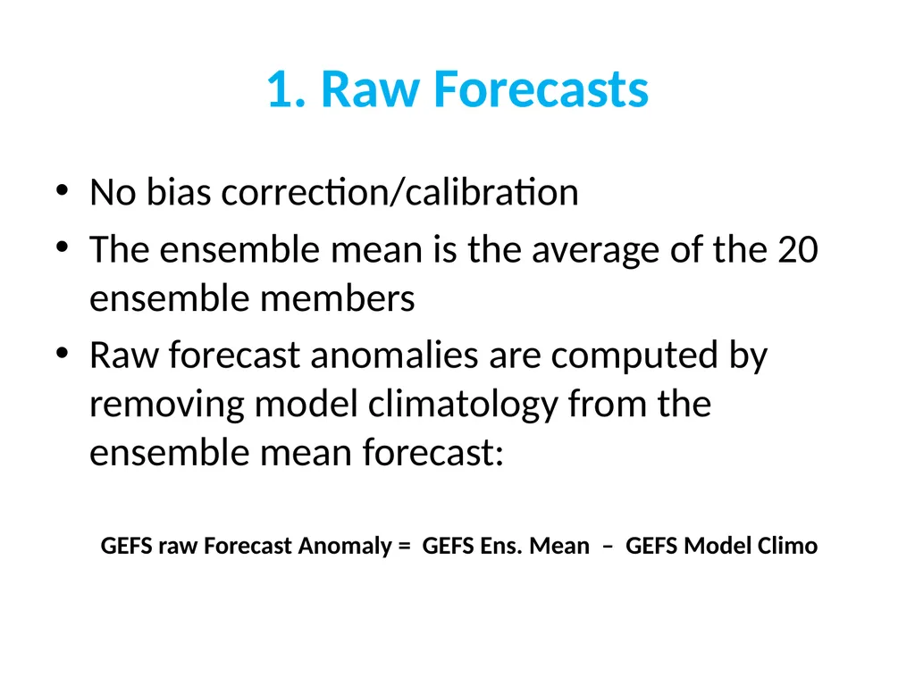
slide2. 1. Raw Forecasts No bias correction/calibration
The ensemble mean is the average of the 20 ensemble members
Raw forecast anomalies are computed by removing model climatology from the ensemble mean forecast:
GEFS raw Forecast Anomaly = GEFS Ens. Mean – GEFS Model Climo<br>
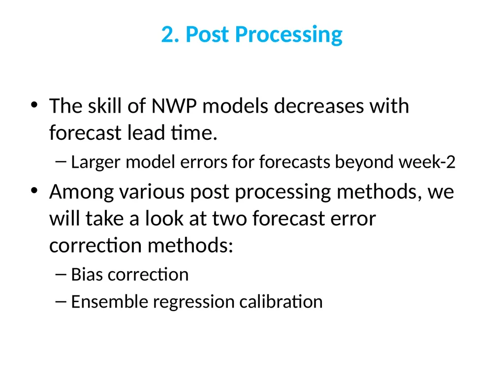
slide3. 2. Post Processing The skill of NWP models decreases with forecast lead time.
Larger model errors for forecasts beyond week-2
Among various post processing methods, we will take a look at two forecast error correction methods:
Bias correction
Ensemble regression calibration<br>
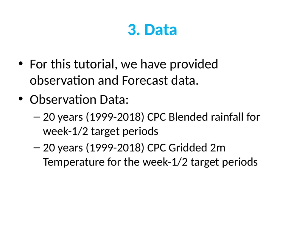
slide4. 3. Data For this tutorial, we have provided observation and Forecast data.
Observation Data:
20 years (1999-2018) CPC Blended rainfall for week-1/2 target periods
20 years (1999-2018) CPC Gridded 2m Temperature for the week-1/2 target periods<br>
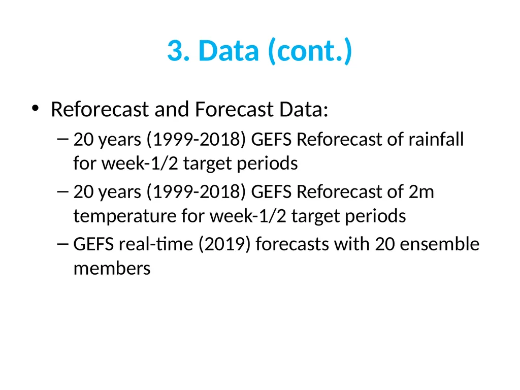
slide5. 3. Data (cont.) Reforecast and Forecast Data:
20 years (1999-2018) GEFS Reforecast of rainfall for week-1/2 target periods
20 years (1999-2018) GEFS Reforecast of 2m temperature for week-1/2 target periods
GEFS real-time (2019) forecasts with 20 ensemble members<br>
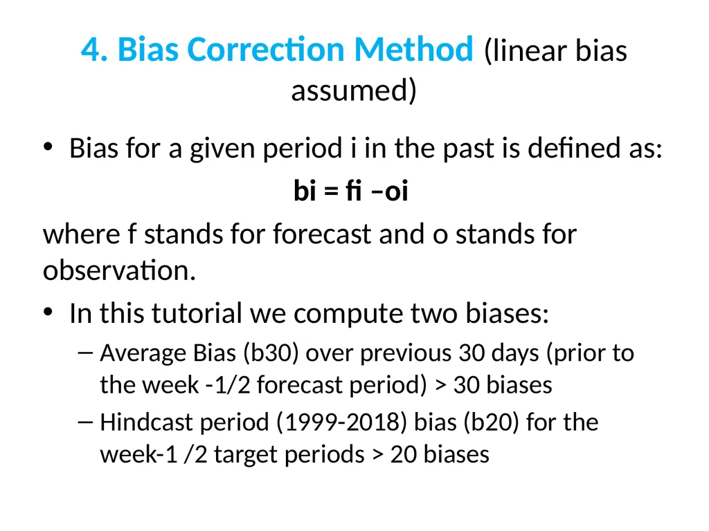
slide6. 4. Bias Correction Method (linear bias assumed) Bias for a given period i in the past is defined as:
bi = fi –oi
where f stands for forecast and o stands for observation.
In this tutorial we compute two biases:
Average Bias (b30) over previous 30 days (prior to the week -1/2 forecast period) > 30 biases
Hindcast period (1999-2018) bias (b20) for the week-1 /2 target periods > 20 biases<br>
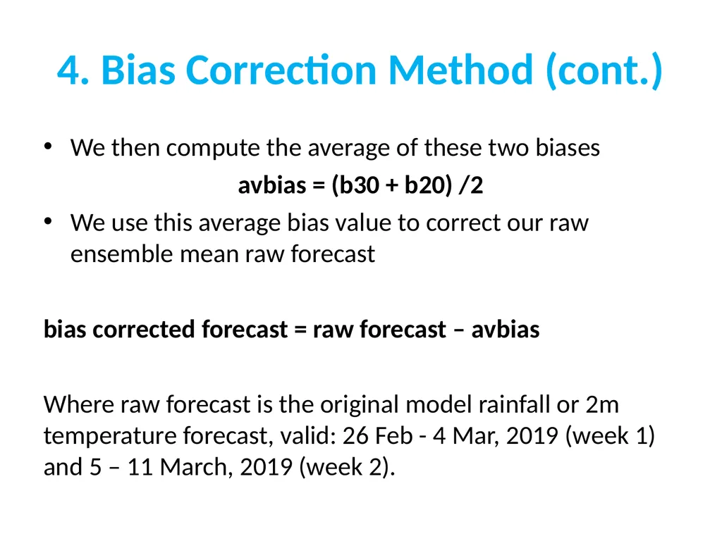
slide7. 4. Bias Correction Method (cont.) We then compute the average of these two biases
avbias = (b30 + b20) /2
We use this average bias value to correct our raw ensemble mean raw forecast
bias corrected forecast = raw forecast – avbias
Where raw forecast is the original model rainfall or 2m temperature forecast, valid: 26 Feb - 4 Mar, 2019 (week 1) and 5 – 11 March, 2019 (week 2).<br>
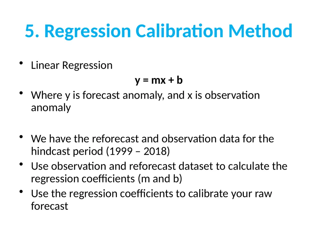
slide8. 5. Regression Calibration Method Linear Regression
y = mx + b
Where y is forecast anomaly, and x is observation anomaly
We have the reforecast and observation data for the hindcast period (1999 – 2018)
Use observation and reforecast dataset to calculate the regression coefficients (m and b)
Use the regression coefficients to calibrate your raw forecast<br>
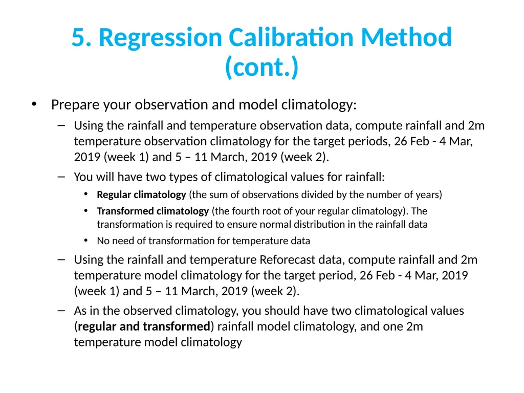
slide9. 5. Regression Calibration Method (cont.) Prepare your observation and model climatology:
Using the rainfall and temperature observation data, compute rainfall and 2m temperature observation climatology for the target periods, 26 Feb - 4 Mar, 2019 (week 1) and 5 – 11 March, 2019 (week 2).
You will have two types of climatological values for rainfall:
Regular climatology (the sum of observations divided by the number of years)
Transformed climatology (the fourth root of your regular climatology). The transformation is required to ensure normal distribution in the rainfall data
No need of transformation for temperature data
Using the rainfall and temperature Reforecast data, compute rainfall and 2m temperature model climatology for the target period, 26 Feb - 4 Mar, 2019 (week 1) and 5 – 11 March, 2019 (week 2).
As in the observed climatology, you should have two climatological values (regular and transformed) rainfall model climatology, and one 2m temperature model climatology<br>
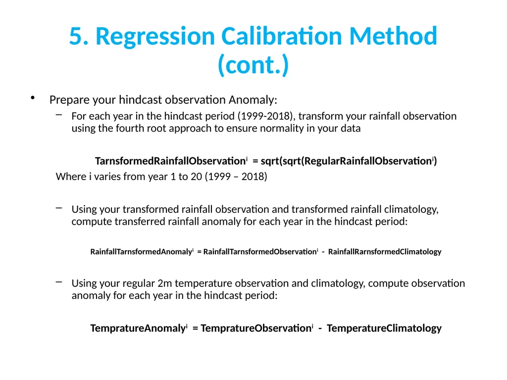
slide10. 5. Regression Calibration Method (cont.) Prepare your hindcast observation Anomaly:
For each year in the hindcast period (1999-2018), transform your rainfall observation using the fourth root approach to ensure normality in your data
TarnsformedRainfallObservationi = sqrt(sqrt(RegularRainfallObservationi)
Where i varies from year 1 to 20 (1999 – 2018)
Using your transformed rainfall observation and transformed rainfall climatology, compute transferred rainfall anomaly for each year in the hindcast period:
RainfallTarnsformedAnomalyi = RainfallTarnsformedObservationi - RainfallRarnsformedClimatology
Using your regular 2m temperature observation and climatology, compute observation anomaly for each year in the hindcast period:
TempratureAnomalyi = TempratureObservationi - TemperatureClimatology<br>
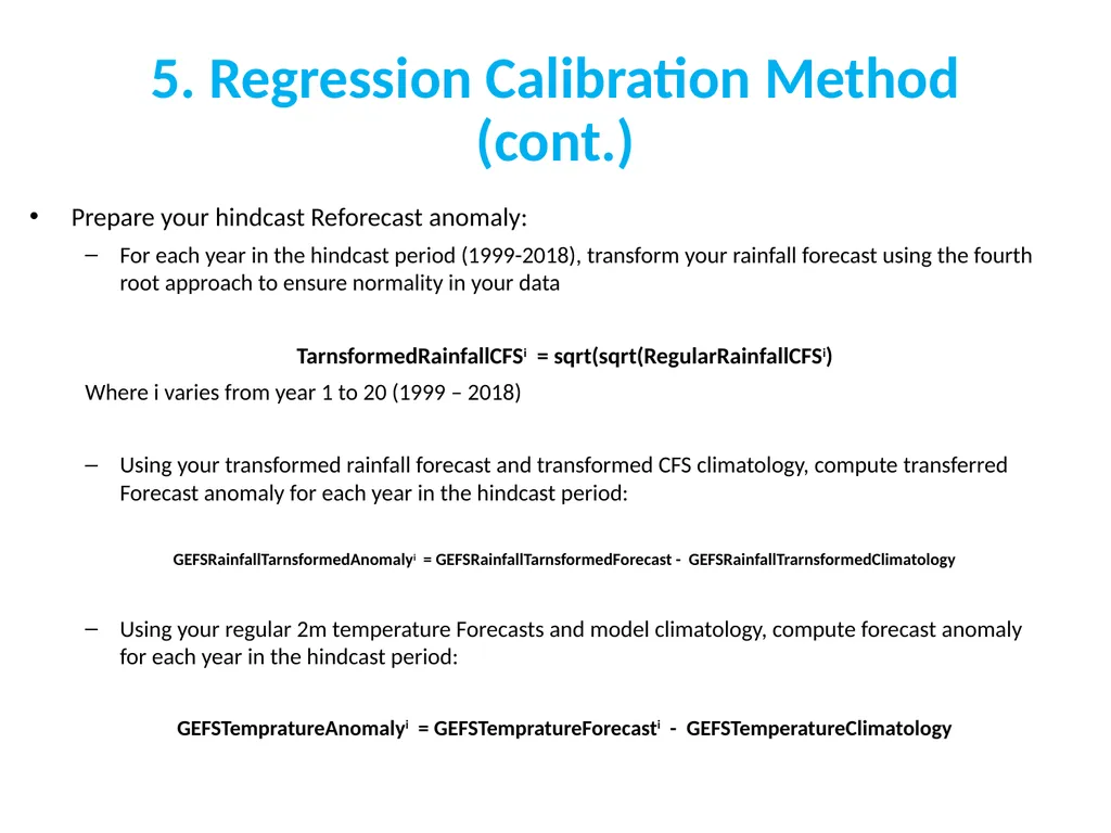
slide11. 5. Regression Calibration Method (cont.) Prepare your hindcast Reforecast anomaly:
For each year in the hindcast period (1999-2018), transform your rainfall forecast using the fourth root approach to ensure normality in your data
TarnsformedRainfallCFSi = sqrt(sqrt(RegularRainfallCFSi)
Where i varies from year 1 to 20 (1999 – 2018)
Using your transformed rainfall forecast and transformed CFS climatology, compute transferred Forecast anomaly for each year in the hindcast period:
GEFSRainfallTarnsformedAnomalyi = GEFSRainfallTarnsformedForecast - GEFSRainfallTrarnsformedClimatology
Using your regular 2m temperature Forecasts and model climatology, compute forecast anomaly for each year in the hindcast period:
GEFSTempratureAnomalyi = GEFSTempratureForecasti - GEFSTemperatureClimatology<br>
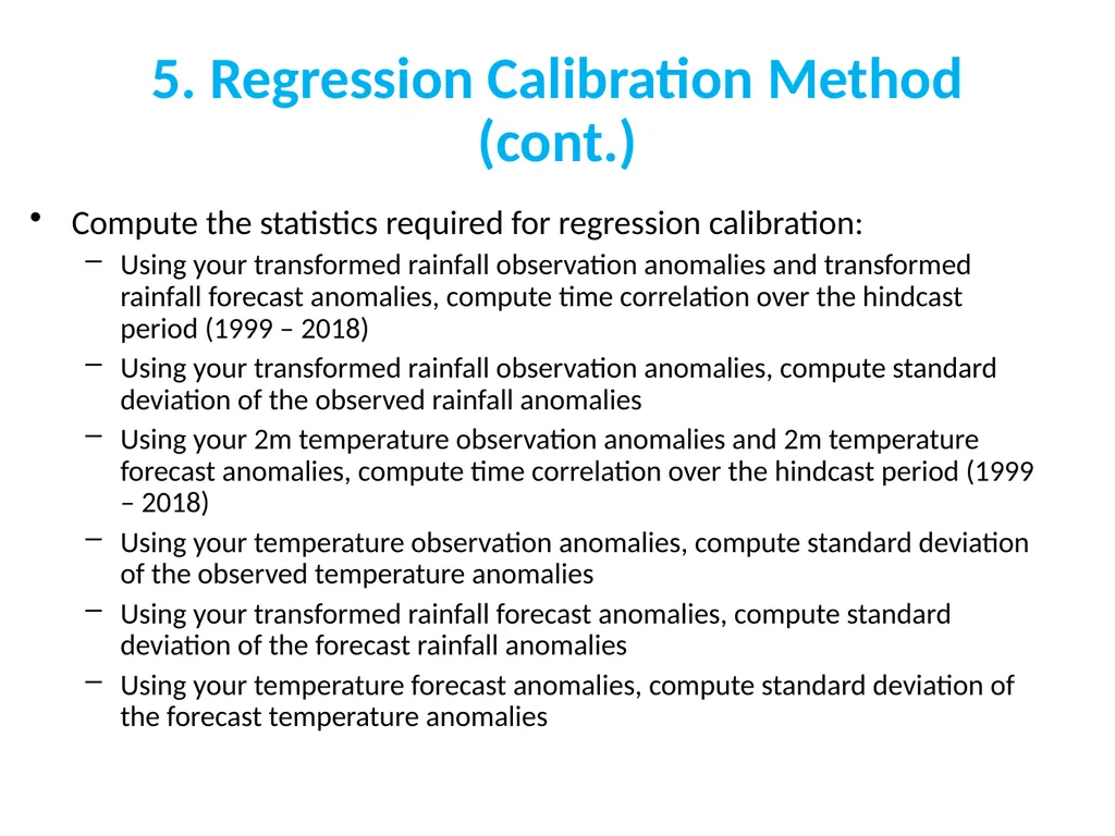
slide12. 5. Regression Calibration Method (cont.) Compute the statistics required for regression calibration:
Using your transformed rainfall observation anomalies and transformed rainfall forecast anomalies, compute time correlation over the hindcast period (1999 – 2018)
Using your transformed rainfall observation anomalies, compute standard deviation of the observed rainfall anomalies
Using your 2m temperature observation anomalies and 2m temperature forecast anomalies, compute time correlation over the hindcast period (1999 – 2018)
Using your temperature observation anomalies, compute standard deviation of the observed temperature anomalies
Using your transformed rainfall forecast anomalies, compute standard deviation of the forecast rainfall anomalies
Using your temperature forecast anomalies, compute standard deviation of the forecast temperature anomalies<br>
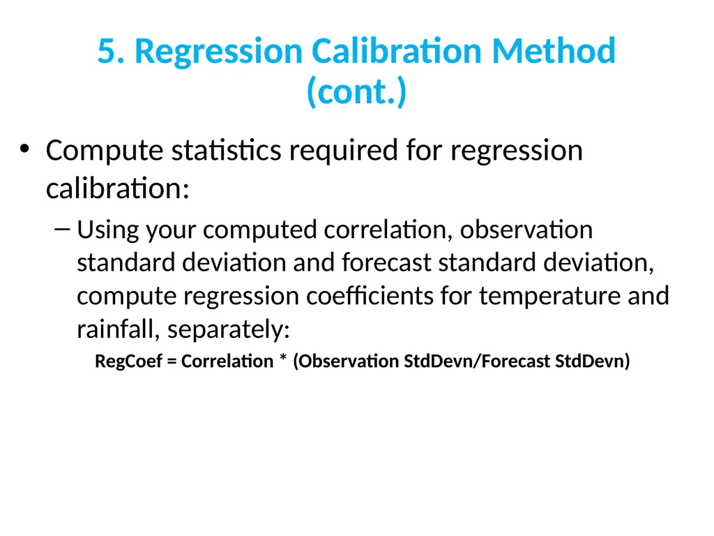
slide13. 5. Regression Calibration Method (cont.) Compute statistics required for regression calibration:
Using your computed correlation, observation standard deviation and forecast standard deviation, compute regression coefficients for temperature and rainfall, separately:
RegCoef = Correlation * (Observation StdDevn/Forecast StdDevn)<br>
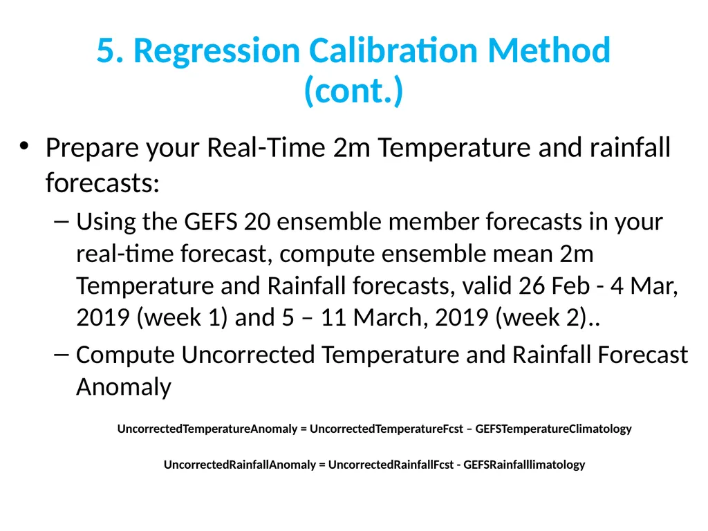
slide14. 5. Regression Calibration Method (cont.) Prepare your Real-Time 2m Temperature and rainfall forecasts:
Using the GEFS 20 ensemble member forecasts in your real-time forecast, compute ensemble mean 2m Temperature and Rainfall forecasts, valid 26 Feb - 4 Mar, 2019 (week 1) and 5 – 11 March, 2019 (week 2)..
Compute Uncorrected Temperature and Rainfall Forecast Anomaly
UncorrectedTemperatureAnomaly = UncorrectedTemperatureFcst – GEFSTemperatureClimatology
UncorrectedRainfallAnomaly = UncorrectedRainfallFcst - GEFSRainfalllimatology<br>
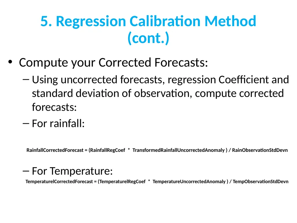
slide15. 5. Regression Calibration Method (cont.) Compute your Corrected Forecasts:
Using uncorrected forecasts, regression Coefficient and standard deviation of observation, compute corrected forecasts:
For rainfall:
RainfallCorrectedForecast = (RainfallRegCoef * TransformedRainfallUncorrectedAnomaly ) / RainObservationStdDevn
For Temperature:
TemperaturelCorrectedForecast = (TemperaturelRegCoef * TemperatureUncorrectedAnomaly ) / TempObservationStdDevn<br>
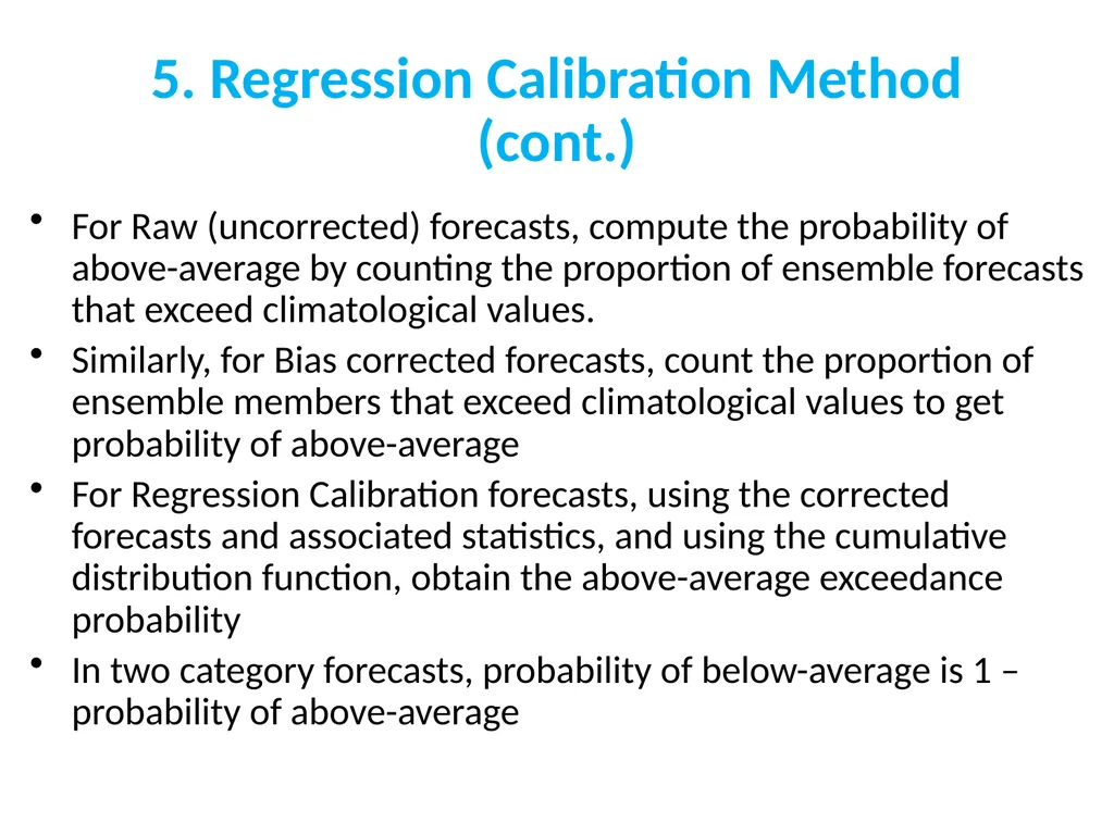
slide16. 5. Regression Calibration Method (cont.) For Raw (uncorrected) forecasts, compute the probability of above-average by counting the proportion of ensemble forecasts that exceed climatological values.
Similarly, for Bias corrected forecasts, count the proportion of ensemble members that exceed climatological values to get probability of above-average
For Regression Calibration forecasts, using the corrected forecasts and associated statistics, and using the cumulative distribution function, obtain the above-average exceedance probability
In two category forecasts, probability of below-average is 1 – probability of above-average<br>
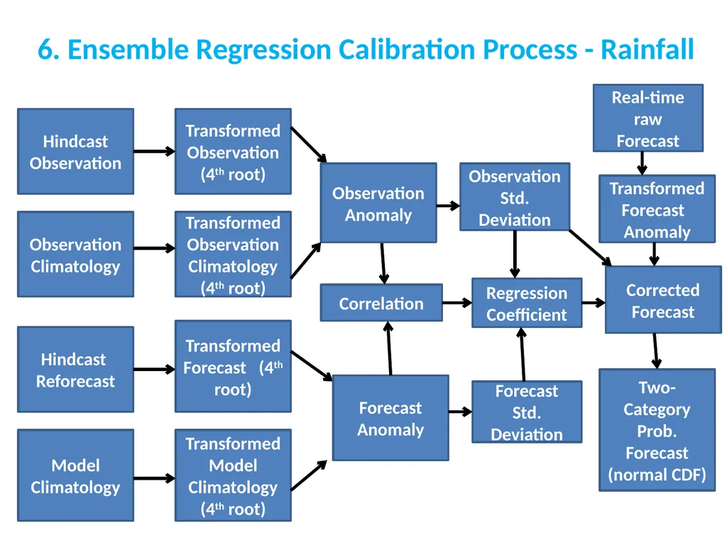
slide17. 6. Ensemble Regression Calibration Process - Rainfall Hindcast Observation Transformed Observation (4th root) Correlation Hindcast Reforecast Observation Climatology Transformed Observation Climatology (4th root) Model Climatology Transformed Forecast (4th root) Transformed Model Climatology (4th root) Observation Anomaly Forecast Anomaly Observation Std. Deviation Forecast Std. Deviation Regression Coefficient Real-time raw Forecast Transformed Forecast Anomaly Corrected Forecast Two-Category Prob. Forecast (normal CDF)<br>
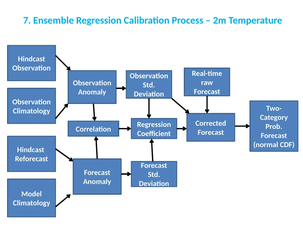
slide18. 7. Ensemble Regression Calibration Process – 2m Temperature Hindcast Observation Correlation Hindcast Reforecast Observation Climatology Model Climatology Observation Anomaly Forecast Anomaly Observation Std. Deviation Forecast Std. Deviation Regression Coefficient Real-time raw Forecast Corrected Forecast Two-Category Prob. Forecast (normal CDF)<br>
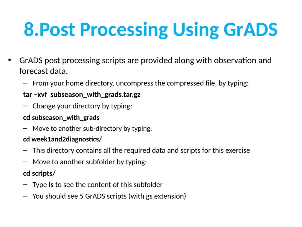
slide19. 8.Post Processing Using GrADS GrADS post processing scripts are provided along with observation and forecast data.
From your home directory, uncompress the compressed file, by typing:
tar –xvf subseason_with_grads.tar.gz
Change your directory by typing:
cd subseason_with_grads
Move to another sub-directory by typing:
cd week1and2diagnostics/
This directory contains all the required data and scripts for this exercise
Move to another subfolder by typing:
cd scripts/
Type ls to see the content of this subfolder
You should see 5 GrADS scripts (with gs extension)<br>
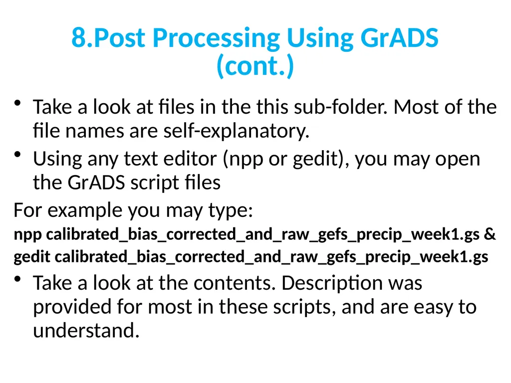
slide20. 8.Post Processing Using GrADS (cont.) Take a look at files in the this sub-folder. Most of the file names are self-explanatory.
Using any text editor (npp or gedit), you may open the GrADS script files
For example you may type:
npp calibrated_bias_corrected_and_raw_gefs_precip_week1.gs &
gedit calibrated_bias_corrected_and_raw_gefs_precip_week1.gs
Take a look at the contents. Description was provided for most in these scripts, and are easy to understand.<br>
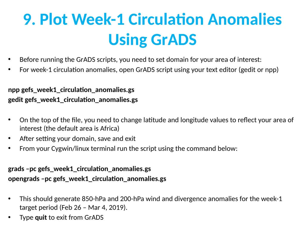
slide21. 9. Plot Week-1 Circulation Anomalies Using GrADS Before running the GrADS scripts, you need to set domain for your area of interest:
For week-1 circulation anomalies, open GrADS script using your text editor (gedit or npp)
npp gefs_week1_circulation_anomalies.gs
gedit gefs_week1_circulation_anomalies.gs
On the top of the file, you need to change latitude and longitude values to reflect your area of interest (the default area is Africa)
After setting your domain, save and exit
From your Cygwin/linux terminal run the script using the command below:
grads –pc gefs_week1_circulation_anomalies.gs
opengrads –pc gefs_week1_circulation_anomalies.gs
This should generate 850-hPa and 200-hPa wind and divergence anomalies for the week-1 target period (Feb 26 – Mar 4, 2019).
Type quit to exit from GrADS<br>
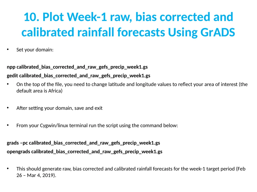
slide22. 10. Plot Week-1 raw, bias corrected and calibrated rainfall forecasts Using GrADS Set your domain:
npp calibrated_bias_corrected_and_raw_gefs_precip_week1.gs
gedit calibrated_bias_corrected_and_raw_gefs_precip_week1.gs
On the top of the file, you need to change latitude and longitude values to reflect your area of interest (the default area is Africa)
After setting your domain, save and exit
From your Cygwin/linux terminal run the script using the command below:
grads –pc calibrated_bias_corrected_and_raw_gefs_precip_week1.gs
opengrads calibrated_bias_corrected_and_raw_gefs_precip_week1.gs
This should generate raw, bias corrected and calibrated rainfall forecasts for the week-1 target period (Feb 26 – Mar 4, 2019).<br>
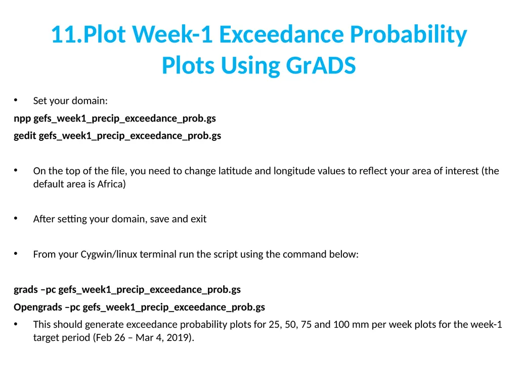
slide23. 11.Plot Week-1 Exceedance Probability Plots Using GrADS Set your domain:
npp gefs_week1_precip_exceedance_prob.gs
gedit gefs_week1_precip_exceedance_prob.gs
On the top of the file, you need to change latitude and longitude values to reflect your area of interest (the default area is Africa)
After setting your domain, save and exit
From your Cygwin/linux terminal run the script using the command below:
grads –pc gefs_week1_precip_exceedance_prob.gs
Opengrads –pc gefs_week1_precip_exceedance_prob.gs
This should generate exceedance probability plots for 25, 50, 75 and 100 mm per week plots for the week-1 target period (Feb 26 – Mar 4, 2019).<br>
slide24. Exercise Run circulation and rainfall anomaly as well as exceedance probability scripts for week 2
Remember to set your domain
Use the images generated from week-2 scripts, together with the MJO information discussed in the morning, create a week-2 diagnostic ppt for your area of interest.<br>
NOAA/CPC/International Desks<br>
slide2. 1. Raw Forecasts No bias correction/calibration
The ensemble mean is the average of the 20 ensemble members
Raw forecast anomalies are computed by removing model climatology from the ensemble mean forecast:
GEFS raw Forecast Anomaly = GEFS Ens. Mean – GEFS Model Climo<br>
slide3. 2. Post Processing The skill of NWP models decreases with forecast lead time.
Larger model errors for forecasts beyond week-2
Among various post processing methods, we will take a look at two forecast error correction methods:
Bias correction
Ensemble regression calibration<br>
slide4. 3. Data For this tutorial, we have provided observation and Forecast data.
Observation Data:
20 years (1999-2018) CPC Blended rainfall for week-1/2 target periods
20 years (1999-2018) CPC Gridded 2m Temperature for the week-1/2 target periods<br>
slide5. 3. Data (cont.) Reforecast and Forecast Data:
20 years (1999-2018) GEFS Reforecast of rainfall for week-1/2 target periods
20 years (1999-2018) GEFS Reforecast of 2m temperature for week-1/2 target periods
GEFS real-time (2019) forecasts with 20 ensemble members<br>
slide6. 4. Bias Correction Method (linear bias assumed) Bias for a given period i in the past is defined as:
bi = fi –oi
where f stands for forecast and o stands for observation.
In this tutorial we compute two biases:
Average Bias (b30) over previous 30 days (prior to the week -1/2 forecast period) > 30 biases
Hindcast period (1999-2018) bias (b20) for the week-1 /2 target periods > 20 biases<br>
slide7. 4. Bias Correction Method (cont.) We then compute the average of these two biases
avbias = (b30 + b20) /2
We use this average bias value to correct our raw ensemble mean raw forecast
bias corrected forecast = raw forecast – avbias
Where raw forecast is the original model rainfall or 2m temperature forecast, valid: 26 Feb - 4 Mar, 2019 (week 1) and 5 – 11 March, 2019 (week 2).<br>
slide8. 5. Regression Calibration Method Linear Regression
y = mx + b
Where y is forecast anomaly, and x is observation anomaly
We have the reforecast and observation data for the hindcast period (1999 – 2018)
Use observation and reforecast dataset to calculate the regression coefficients (m and b)
Use the regression coefficients to calibrate your raw forecast<br>
slide9. 5. Regression Calibration Method (cont.) Prepare your observation and model climatology:
Using the rainfall and temperature observation data, compute rainfall and 2m temperature observation climatology for the target periods, 26 Feb - 4 Mar, 2019 (week 1) and 5 – 11 March, 2019 (week 2).
You will have two types of climatological values for rainfall:
Regular climatology (the sum of observations divided by the number of years)
Transformed climatology (the fourth root of your regular climatology). The transformation is required to ensure normal distribution in the rainfall data
No need of transformation for temperature data
Using the rainfall and temperature Reforecast data, compute rainfall and 2m temperature model climatology for the target period, 26 Feb - 4 Mar, 2019 (week 1) and 5 – 11 March, 2019 (week 2).
As in the observed climatology, you should have two climatological values (regular and transformed) rainfall model climatology, and one 2m temperature model climatology<br>
slide10. 5. Regression Calibration Method (cont.) Prepare your hindcast observation Anomaly:
For each year in the hindcast period (1999-2018), transform your rainfall observation using the fourth root approach to ensure normality in your data
TarnsformedRainfallObservationi = sqrt(sqrt(RegularRainfallObservationi)
Where i varies from year 1 to 20 (1999 – 2018)
Using your transformed rainfall observation and transformed rainfall climatology, compute transferred rainfall anomaly for each year in the hindcast period:
RainfallTarnsformedAnomalyi = RainfallTarnsformedObservationi - RainfallRarnsformedClimatology
Using your regular 2m temperature observation and climatology, compute observation anomaly for each year in the hindcast period:
TempratureAnomalyi = TempratureObservationi - TemperatureClimatology<br>
slide11. 5. Regression Calibration Method (cont.) Prepare your hindcast Reforecast anomaly:
For each year in the hindcast period (1999-2018), transform your rainfall forecast using the fourth root approach to ensure normality in your data
TarnsformedRainfallCFSi = sqrt(sqrt(RegularRainfallCFSi)
Where i varies from year 1 to 20 (1999 – 2018)
Using your transformed rainfall forecast and transformed CFS climatology, compute transferred Forecast anomaly for each year in the hindcast period:
GEFSRainfallTarnsformedAnomalyi = GEFSRainfallTarnsformedForecast - GEFSRainfallTrarnsformedClimatology
Using your regular 2m temperature Forecasts and model climatology, compute forecast anomaly for each year in the hindcast period:
GEFSTempratureAnomalyi = GEFSTempratureForecasti - GEFSTemperatureClimatology<br>
slide12. 5. Regression Calibration Method (cont.) Compute the statistics required for regression calibration:
Using your transformed rainfall observation anomalies and transformed rainfall forecast anomalies, compute time correlation over the hindcast period (1999 – 2018)
Using your transformed rainfall observation anomalies, compute standard deviation of the observed rainfall anomalies
Using your 2m temperature observation anomalies and 2m temperature forecast anomalies, compute time correlation over the hindcast period (1999 – 2018)
Using your temperature observation anomalies, compute standard deviation of the observed temperature anomalies
Using your transformed rainfall forecast anomalies, compute standard deviation of the forecast rainfall anomalies
Using your temperature forecast anomalies, compute standard deviation of the forecast temperature anomalies<br>
slide13. 5. Regression Calibration Method (cont.) Compute statistics required for regression calibration:
Using your computed correlation, observation standard deviation and forecast standard deviation, compute regression coefficients for temperature and rainfall, separately:
RegCoef = Correlation * (Observation StdDevn/Forecast StdDevn)<br>
slide14. 5. Regression Calibration Method (cont.) Prepare your Real-Time 2m Temperature and rainfall forecasts:
Using the GEFS 20 ensemble member forecasts in your real-time forecast, compute ensemble mean 2m Temperature and Rainfall forecasts, valid 26 Feb - 4 Mar, 2019 (week 1) and 5 – 11 March, 2019 (week 2)..
Compute Uncorrected Temperature and Rainfall Forecast Anomaly
UncorrectedTemperatureAnomaly = UncorrectedTemperatureFcst – GEFSTemperatureClimatology
UncorrectedRainfallAnomaly = UncorrectedRainfallFcst - GEFSRainfalllimatology<br>
slide15. 5. Regression Calibration Method (cont.) Compute your Corrected Forecasts:
Using uncorrected forecasts, regression Coefficient and standard deviation of observation, compute corrected forecasts:
For rainfall:
RainfallCorrectedForecast = (RainfallRegCoef * TransformedRainfallUncorrectedAnomaly ) / RainObservationStdDevn
For Temperature:
TemperaturelCorrectedForecast = (TemperaturelRegCoef * TemperatureUncorrectedAnomaly ) / TempObservationStdDevn<br>
slide16. 5. Regression Calibration Method (cont.) For Raw (uncorrected) forecasts, compute the probability of above-average by counting the proportion of ensemble forecasts that exceed climatological values.
Similarly, for Bias corrected forecasts, count the proportion of ensemble members that exceed climatological values to get probability of above-average
For Regression Calibration forecasts, using the corrected forecasts and associated statistics, and using the cumulative distribution function, obtain the above-average exceedance probability
In two category forecasts, probability of below-average is 1 – probability of above-average<br>
slide17. 6. Ensemble Regression Calibration Process - Rainfall Hindcast Observation Transformed Observation (4th root) Correlation Hindcast Reforecast Observation Climatology Transformed Observation Climatology (4th root) Model Climatology Transformed Forecast (4th root) Transformed Model Climatology (4th root) Observation Anomaly Forecast Anomaly Observation Std. Deviation Forecast Std. Deviation Regression Coefficient Real-time raw Forecast Transformed Forecast Anomaly Corrected Forecast Two-Category Prob. Forecast (normal CDF)<br>
slide18. 7. Ensemble Regression Calibration Process – 2m Temperature Hindcast Observation Correlation Hindcast Reforecast Observation Climatology Model Climatology Observation Anomaly Forecast Anomaly Observation Std. Deviation Forecast Std. Deviation Regression Coefficient Real-time raw Forecast Corrected Forecast Two-Category Prob. Forecast (normal CDF)<br>
slide19. 8.Post Processing Using GrADS GrADS post processing scripts are provided along with observation and forecast data.
From your home directory, uncompress the compressed file, by typing:
tar –xvf subseason_with_grads.tar.gz
Change your directory by typing:
cd subseason_with_grads
Move to another sub-directory by typing:
cd week1and2diagnostics/
This directory contains all the required data and scripts for this exercise
Move to another subfolder by typing:
cd scripts/
Type ls to see the content of this subfolder
You should see 5 GrADS scripts (with gs extension)<br>
slide20. 8.Post Processing Using GrADS (cont.) Take a look at files in the this sub-folder. Most of the file names are self-explanatory.
Using any text editor (npp or gedit), you may open the GrADS script files
For example you may type:
npp calibrated_bias_corrected_and_raw_gefs_precip_week1.gs &
gedit calibrated_bias_corrected_and_raw_gefs_precip_week1.gs
Take a look at the contents. Description was provided for most in these scripts, and are easy to understand.<br>
slide21. 9. Plot Week-1 Circulation Anomalies Using GrADS Before running the GrADS scripts, you need to set domain for your area of interest:
For week-1 circulation anomalies, open GrADS script using your text editor (gedit or npp)
npp gefs_week1_circulation_anomalies.gs
gedit gefs_week1_circulation_anomalies.gs
On the top of the file, you need to change latitude and longitude values to reflect your area of interest (the default area is Africa)
After setting your domain, save and exit
From your Cygwin/linux terminal run the script using the command below:
grads –pc gefs_week1_circulation_anomalies.gs
opengrads –pc gefs_week1_circulation_anomalies.gs
This should generate 850-hPa and 200-hPa wind and divergence anomalies for the week-1 target period (Feb 26 – Mar 4, 2019).
Type quit to exit from GrADS<br>
slide22. 10. Plot Week-1 raw, bias corrected and calibrated rainfall forecasts Using GrADS Set your domain:
npp calibrated_bias_corrected_and_raw_gefs_precip_week1.gs
gedit calibrated_bias_corrected_and_raw_gefs_precip_week1.gs
On the top of the file, you need to change latitude and longitude values to reflect your area of interest (the default area is Africa)
After setting your domain, save and exit
From your Cygwin/linux terminal run the script using the command below:
grads –pc calibrated_bias_corrected_and_raw_gefs_precip_week1.gs
opengrads calibrated_bias_corrected_and_raw_gefs_precip_week1.gs
This should generate raw, bias corrected and calibrated rainfall forecasts for the week-1 target period (Feb 26 – Mar 4, 2019).<br>
slide23. 11.Plot Week-1 Exceedance Probability Plots Using GrADS Set your domain:
npp gefs_week1_precip_exceedance_prob.gs
gedit gefs_week1_precip_exceedance_prob.gs
On the top of the file, you need to change latitude and longitude values to reflect your area of interest (the default area is Africa)
After setting your domain, save and exit
From your Cygwin/linux terminal run the script using the command below:
grads –pc gefs_week1_precip_exceedance_prob.gs
Opengrads –pc gefs_week1_precip_exceedance_prob.gs
This should generate exceedance probability plots for 25, 50, 75 and 100 mm per week plots for the week-1 target period (Feb 26 – Mar 4, 2019).<br>
slide24. Exercise Run circulation and rainfall anomaly as well as exceedance probability scripts for week 2
Remember to set your domain
Use the images generated from week-2 scripts, together with the MJO information discussed in the morning, create a week-2 diagnostic ppt for your area of interest.<br>