Probability and Statistics for Computer Scientists

slide1. Probability and Statistics for Computer ScientistsThird Edition, By Michael BaronChapter 3: Discrete Random Variables and Their DistributionsCIS 2033. Computational Probability and Statistics Pei Wang<br>
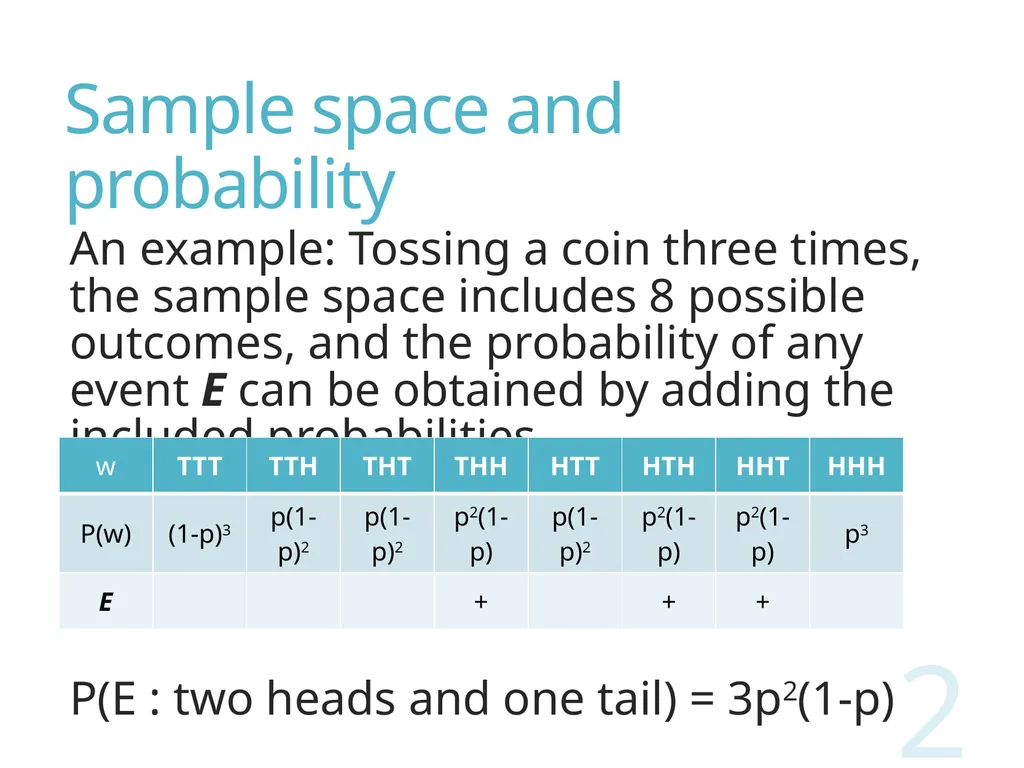
slide2. Sample space and probability An example: Tossing a coin three times, the sample space includes 8 possible outcomes, and the probability of any event E can be obtained by adding the included probabilities

P(E : two heads and one tail) = 3p2(1-p) 2<br>
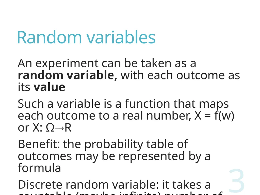
slide3. Random variables An experiment can be taken as a random variable, with each outcome as its value
Such a variable is a function that maps each outcome to a real number, X = f(w) or X: ΩR
Benefit: the probability table of outcomes may be represented by a formula
Discrete random variable: it takes a countable (maybe infinite) number of values 3<br>
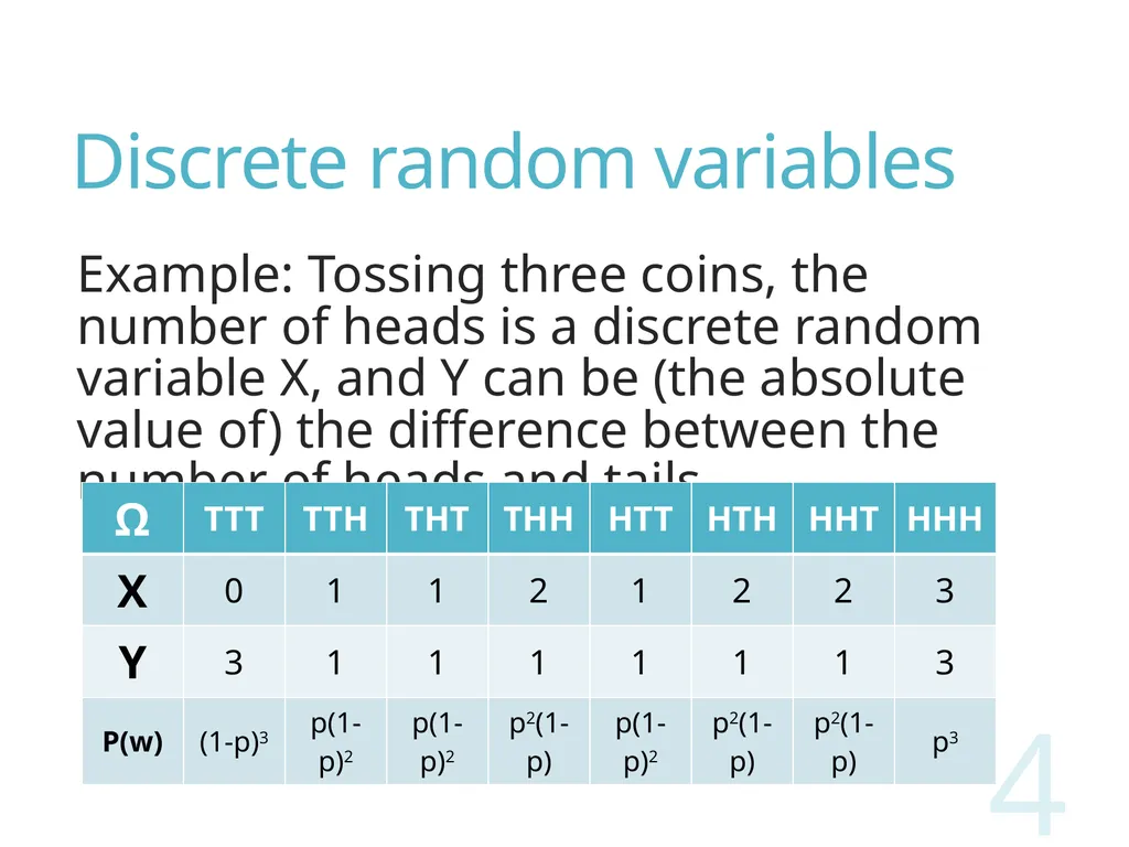
slide4. Discrete random variables Example: Tossing three coins, the number of heads is a discrete random variable X, and Y can be (the absolute value of) the difference between the number of heads and tails 4<br>
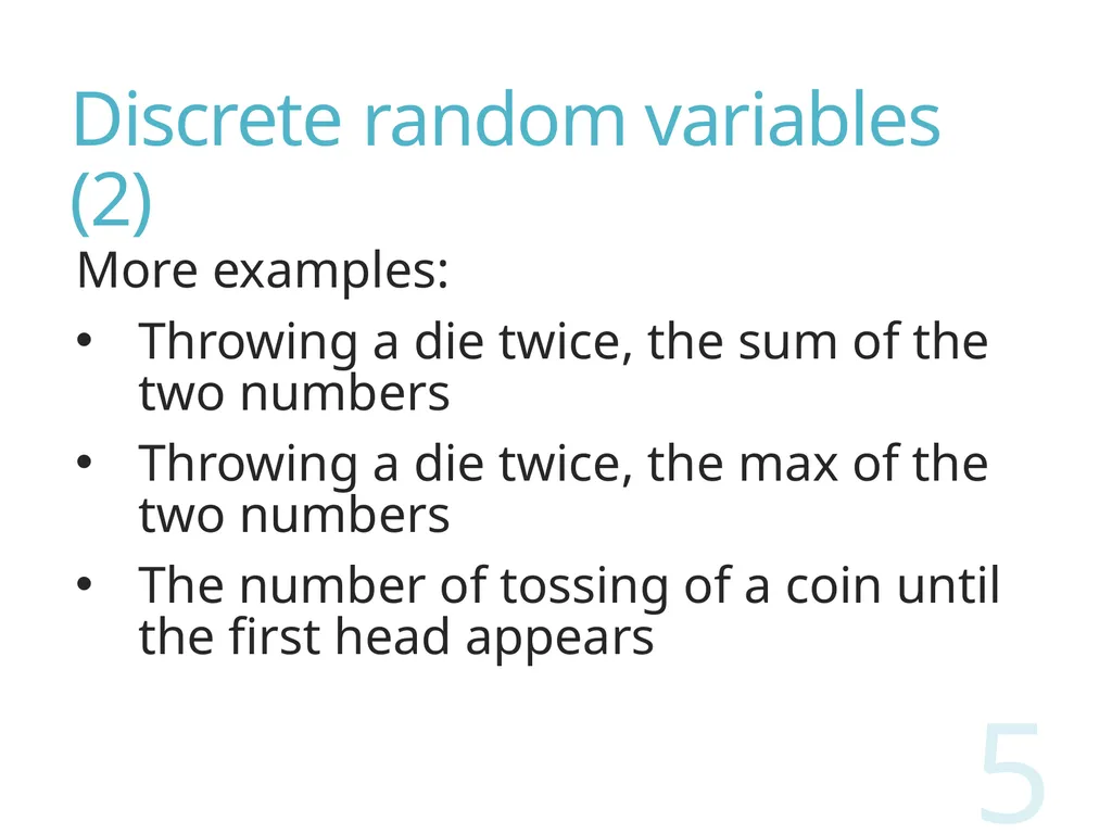
slide5. Discrete random variables (2) More examples:
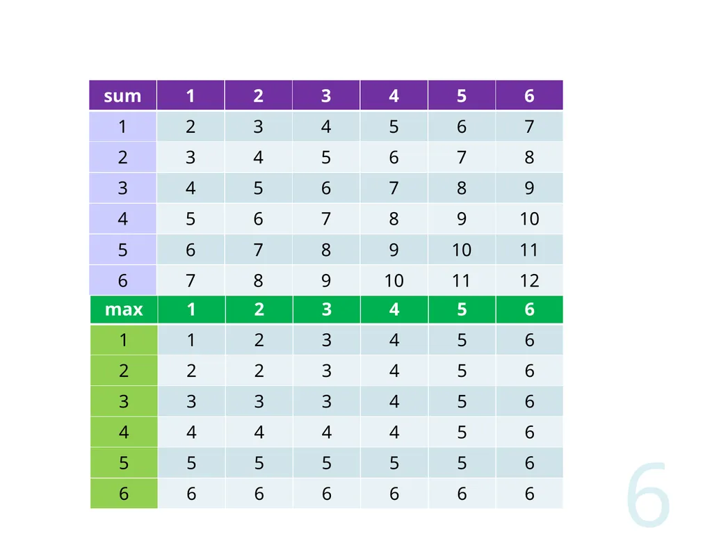
Throwing a die twice, the sum of the two numbers
Throwing a die twice, the max of the two numbers
The number of tossing of a coin until the first head appears 5<br>
slide6. 6<br>
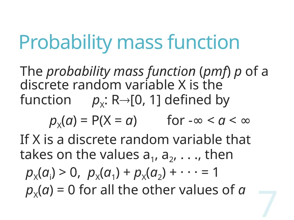
slide7. Probability mass function The probability mass function (pmf) p of a discrete random variable X is the function pX: R[0, 1] defined by
pX(a) = P(X = a) for -∞ < a < ∞
If X is a discrete random variable that takes on the values a1, a2, . . ., then
pX(ai) > 0, pX(a1) + pX(a2) + · · · = 1
pX(a) = 0 for all the other values of a 7<br>
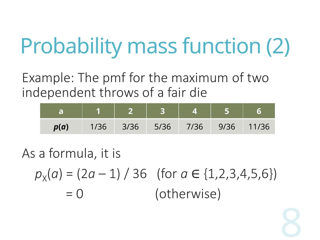
slide8. Probability mass function (2) 8<br>
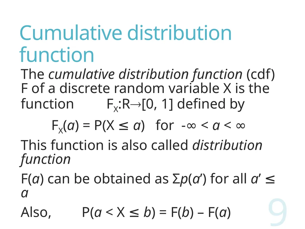
slide9. Cumulative distribution function The cumulative distribution function (cdf) F of a discrete random variable X is the function FX:R[0, 1] defined by
FX(a) = P(X ≤ a) for -∞ < a < ∞
This function is also called distribution function
F(a) can be obtained as Ʃp(a’) for all a’ ≤ a
Also, P(a < X ≤ b) = F(b) – F(a) 9<br>
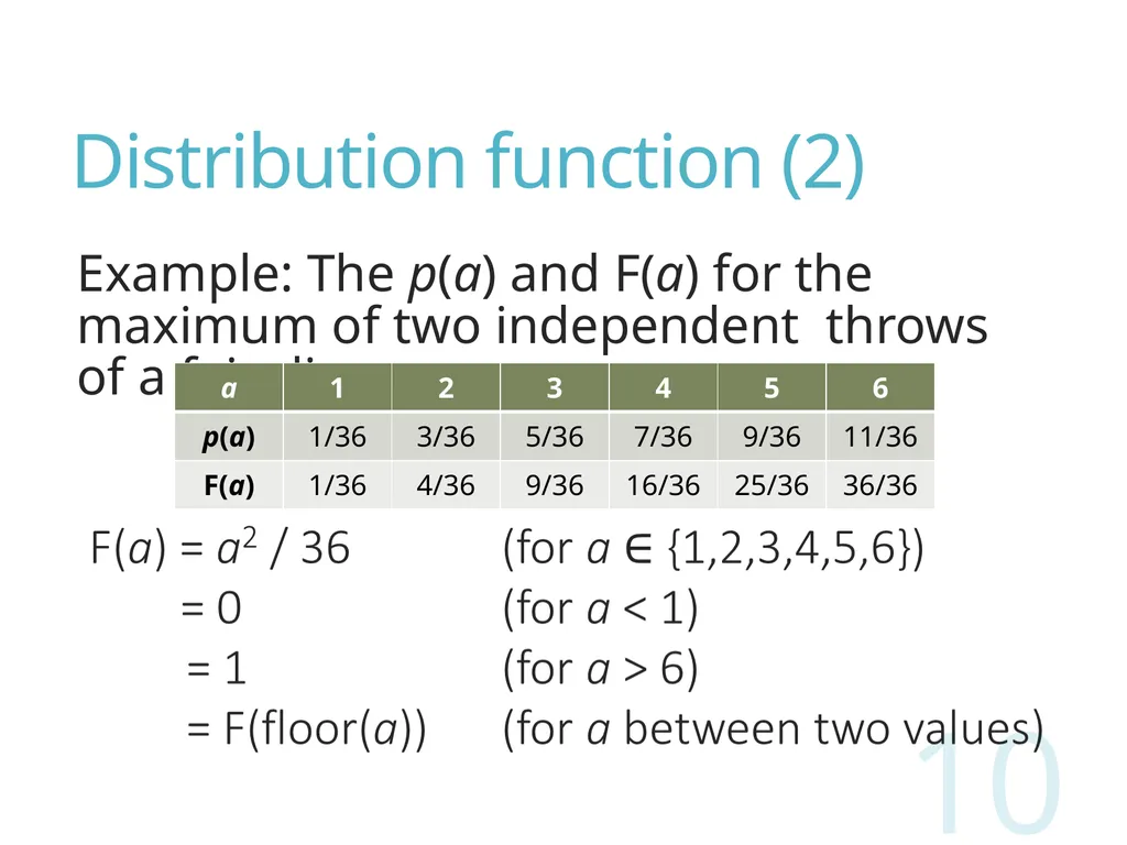
slide10. Distribution function (2) Example: The p(a) and F(a) for the maximum of two independent throws of a fair die 10<br>
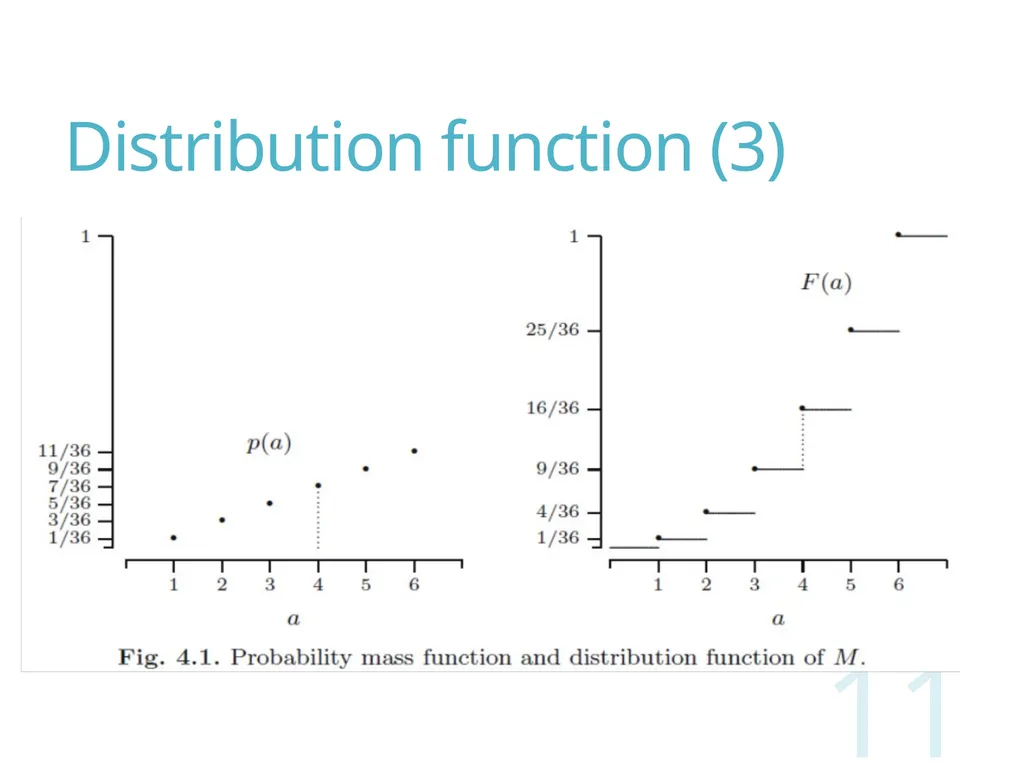
slide11. Distribution function (3) 11<br>
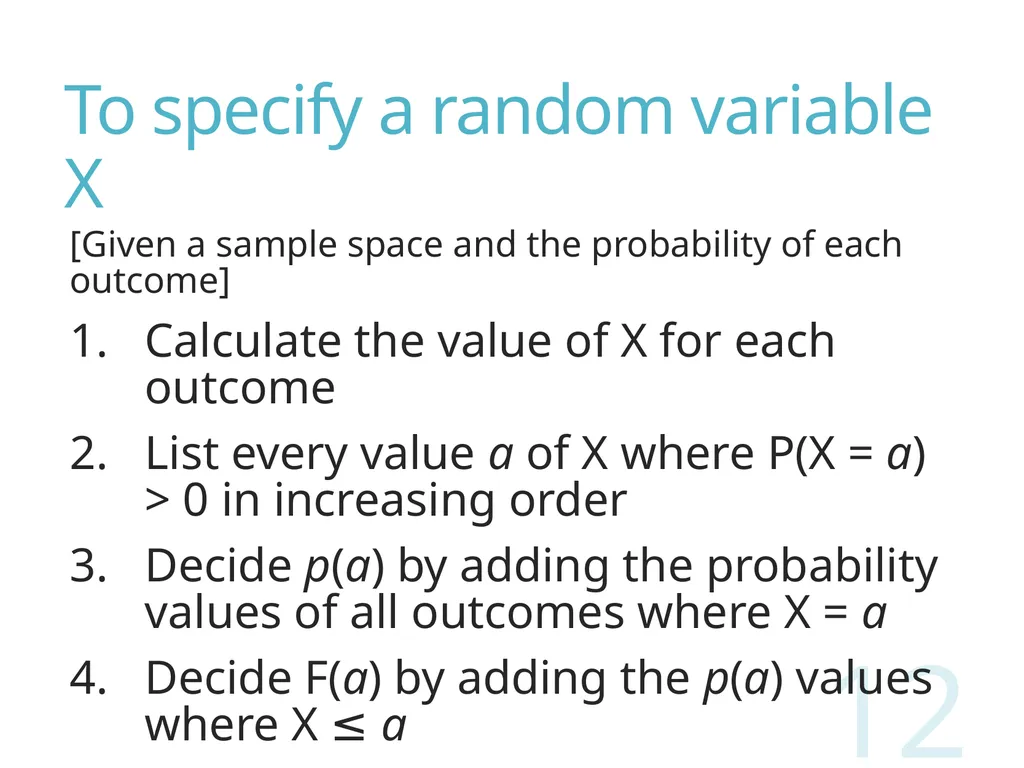
slide12. To specify a random variable X [Given a sample space and the probability of each outcome]
Calculate the value of X for each outcome
List every value a of X where P(X = a) > 0 in increasing order
Decide p(a) by adding the probability values of all outcomes where X = a
Decide F(a) by adding the p(a) values where X ≤ a 12<br>
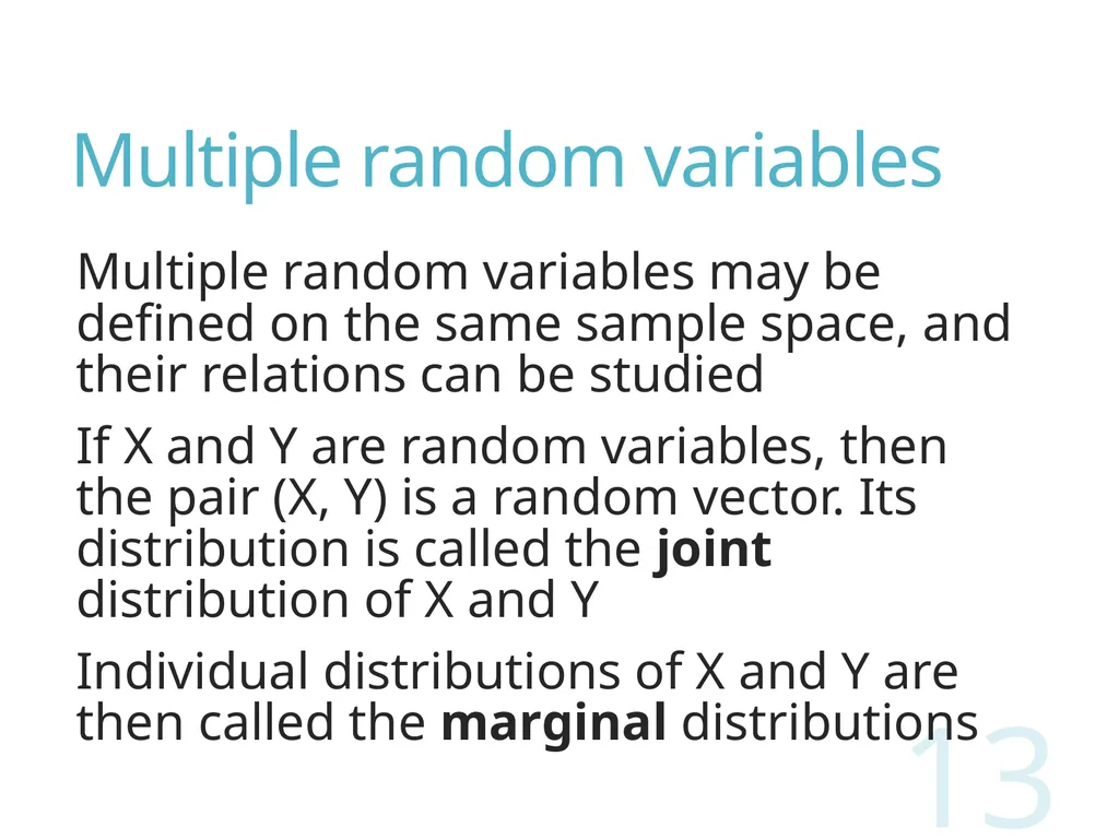
slide13. Multiple random variables Multiple random variables may be defined on the same sample space, and their relations can be studied
If X and Y are random variables, then the pair (X, Y) is a random vector. Its distribution is called the joint distribution of X and Y
Individual distributions of X and Y are then called the marginal distributions 13<br>
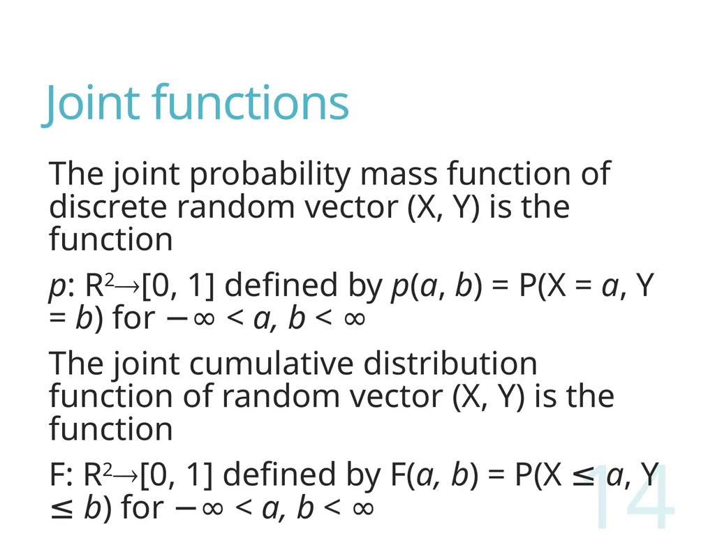
slide14. Joint functions The joint probability mass function of discrete random vector (X, Y) is the function
p: R2[0, 1] defined by p(a, b) = P(X = a, Y = b) for −∞ < a, b < ∞
The joint cumulative distribution function of random vector (X, Y) is the function
F: R2[0, 1] defined by F(a, b) = P(X ≤ a, Y ≤ b) for −∞ < a, b < ∞ 14<br>
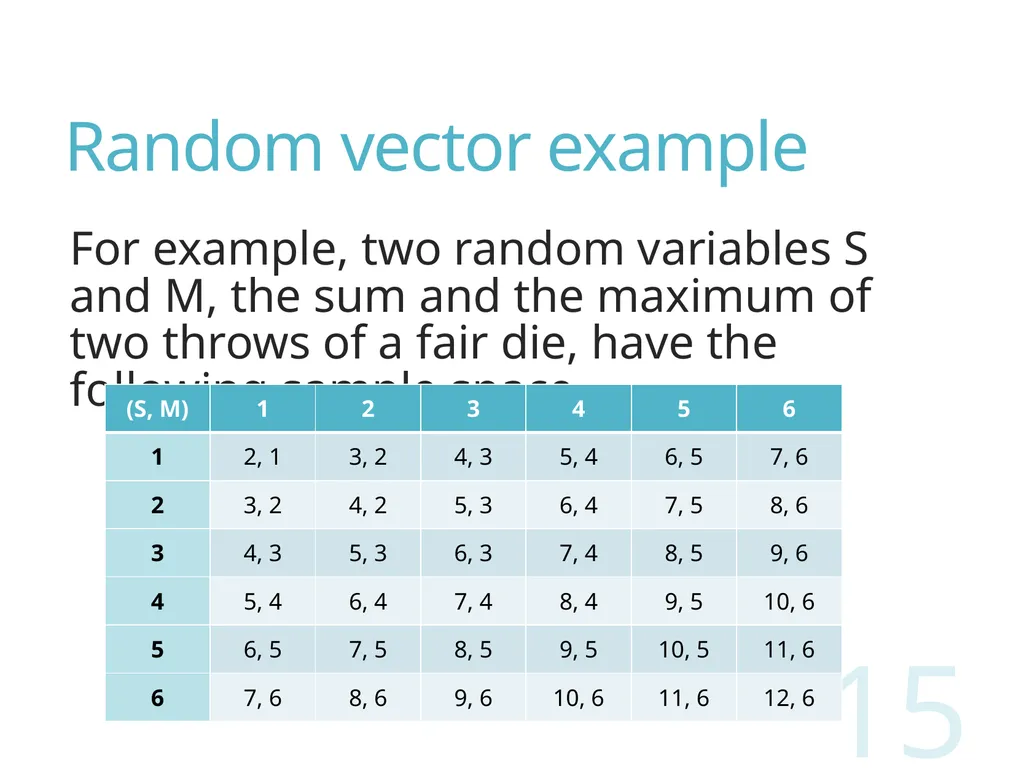
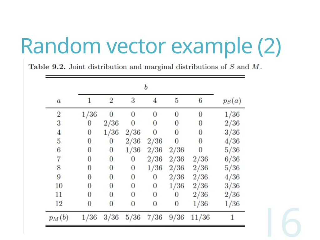
slide15. Random vector example For example, two random variables S and M, the sum and the maximum of two throws of a fair die, have the following sample space 15<br>
slide16. Random vector example (2) 16<br>
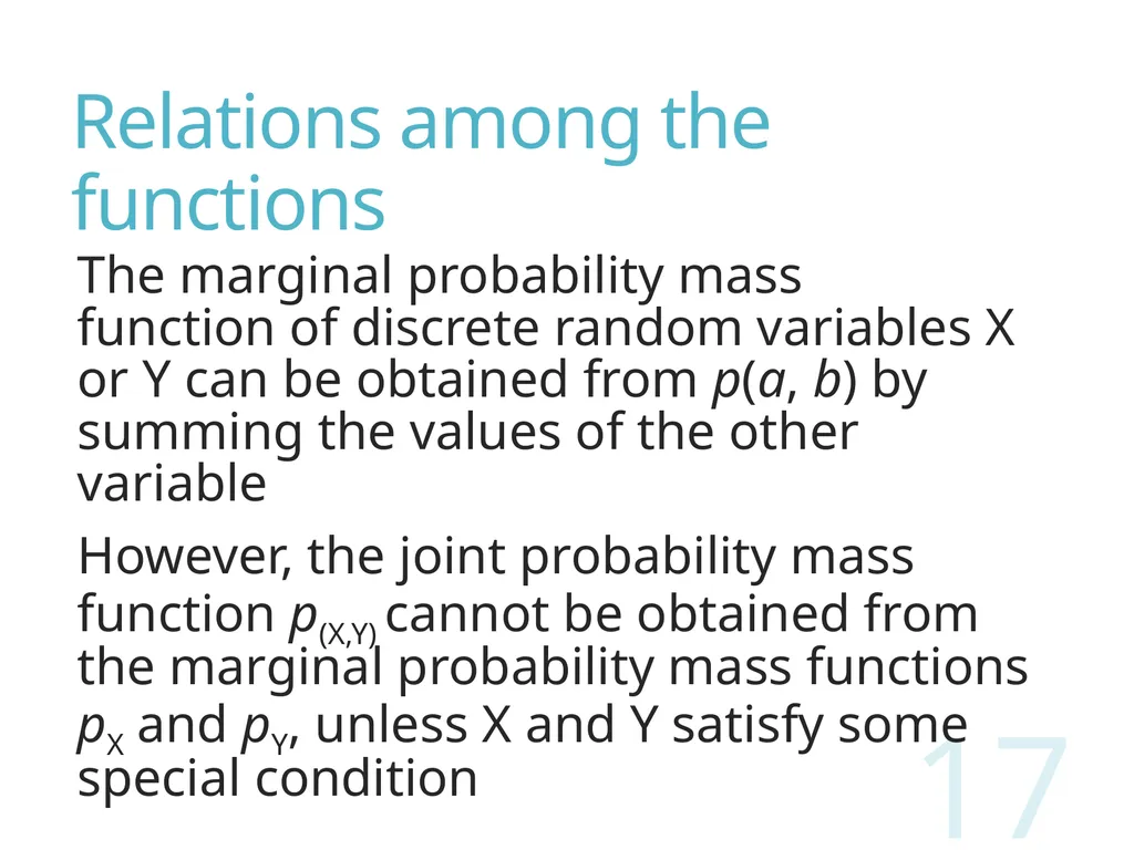
slide17. Relations among the functions The marginal probability mass function of discrete random variables X or Y can be obtained from p(a, b) by summing the values of the other variable
However, the joint probability mass function p(X,Y) cannot be obtained from the marginal probability mass functions pX and pY, unless X and Y satisfy some special condition 17<br>
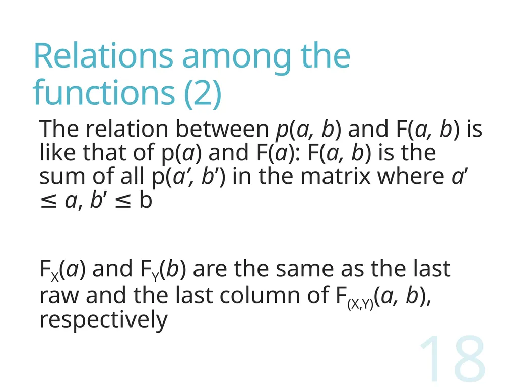
slide18. Relations among the functions (2) The relation between p(a, b) and F(a, b) is like that of p(a) and F(a): F(a, b) is the sum of all p(a’, b’) in the matrix where a’ ≤ a, b’ ≤ b

FX(a) and FY(b) are the same as the last raw and the last column of F(X,Y)(a, b), respectively 18<br>
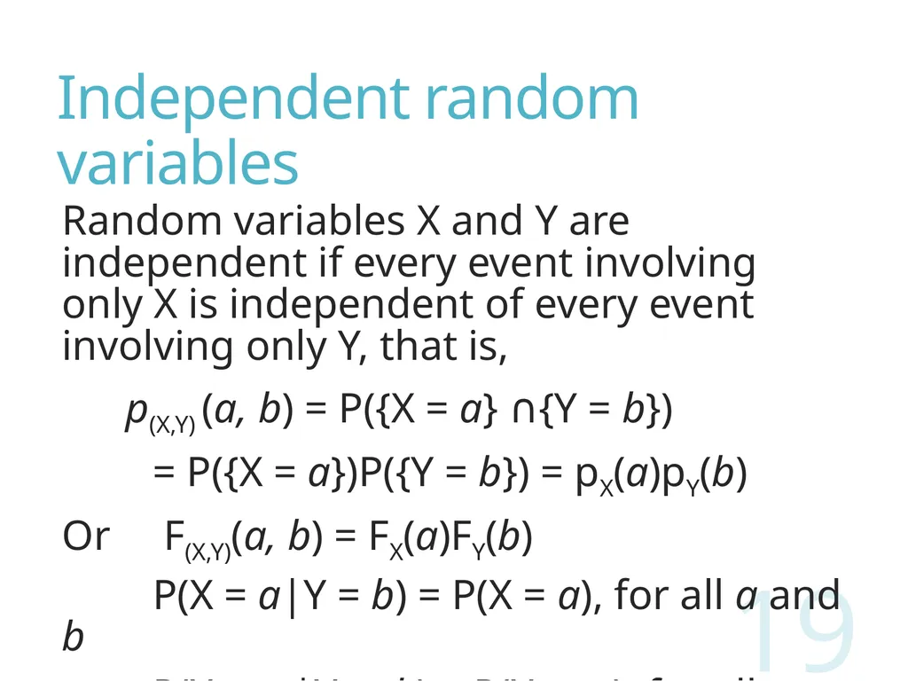
slide19. Independent random variables Random variables X and Y are independent if every event involving only X is independent of every event involving only Y, that is,
      p(X,Y) (a, b) = P({X = a} ∩{Y = b})
= P({X = a})P({Y = b}) = pX(a)pY(b)
Or F(X,Y)(a, b) = FX(a)FY(b)
P(X = a|Y = b) = P(X = a), for all a and b
P(X ≤ a|Y ≤ b) = P(X ≤ a), for all a and b 19<br>
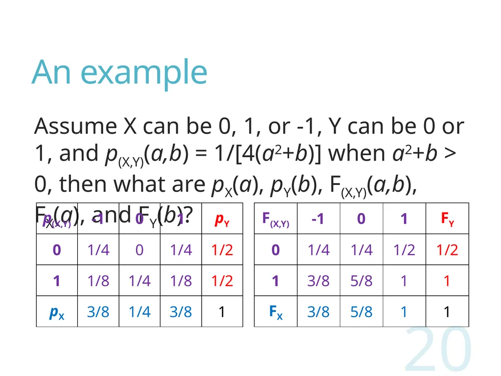
slide20. An example Assume X can be 0, 1, or -1, Y can be 0 or 1, and p(X,Y)(a,b) = 1/[4(a2+b)] when a2+b > 0, then what are pX(a), pY(b), F(X,Y)(a,b), FX(a), and FY(b)? 20<br>
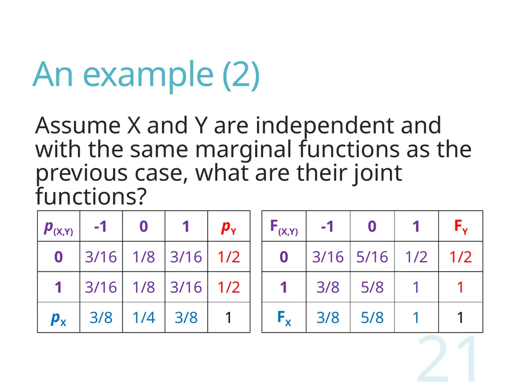
slide21. An example (2) Assume X and Y are independent and with the same marginal functions as the previous case, what are their joint functions? 21<br>
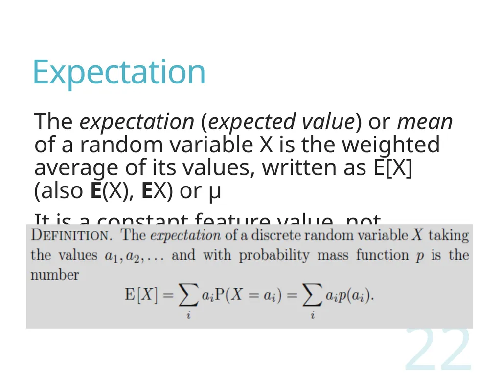
slide22. Expectation The expectation (expected value) or mean of a random variable X is the weighted average of its values, written as E[X] (also E(X), EX) or µ
It is a constant feature value, not random 22<br>
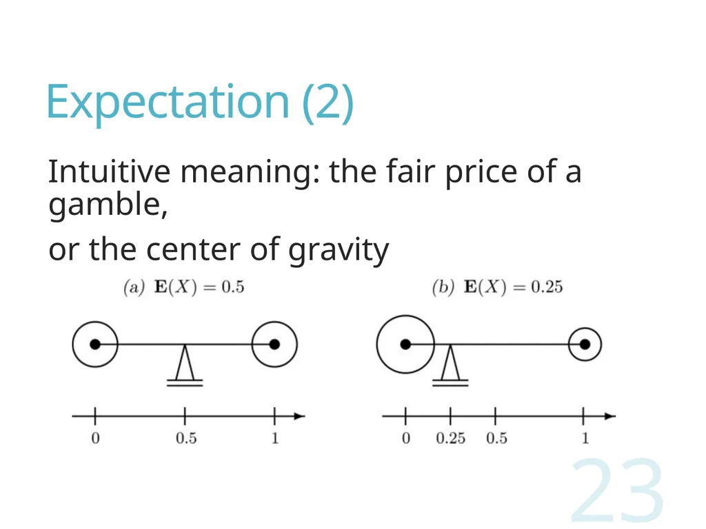
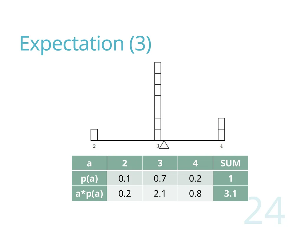
slide23. Expectation (2) Intuitive meaning: the fair price of a gamble,
or the center of gravity 23<br>
slide24. Expectation (3) 24<br>
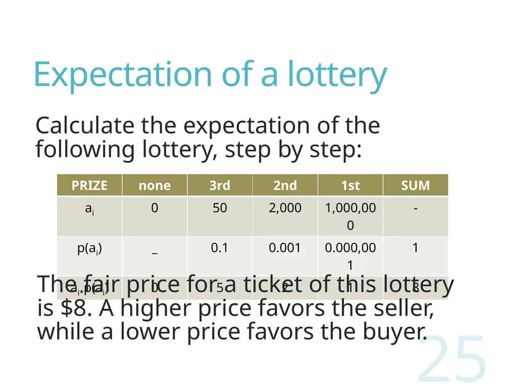
slide25. Expectation of a lottery Calculate the expectation of the following lottery, step by step: 25 The fair price for a ticket of this lottery is $8. A higher price favors the seller, while a lower price favors the buyer.<br>
slide26. Expectation of a lottery (2) Between two lotteries, how to decide which one to choose if their awards are A1 and A2, and probabilities of winning are p1 and p2, respectively?
What if a lottery has multiple awards?
What if their ticket prices are t1 and t2, respectively? 26<br>
slide27. Properties of expectation If the n values are equally probable, the expectation is their average (Ʃai)/n
The expectation of a discrete random variable may not be a valid value of the variable
The expectation may not be exactly at the half-way between the min value and the max value, though it is always in [min, max] 27<br>
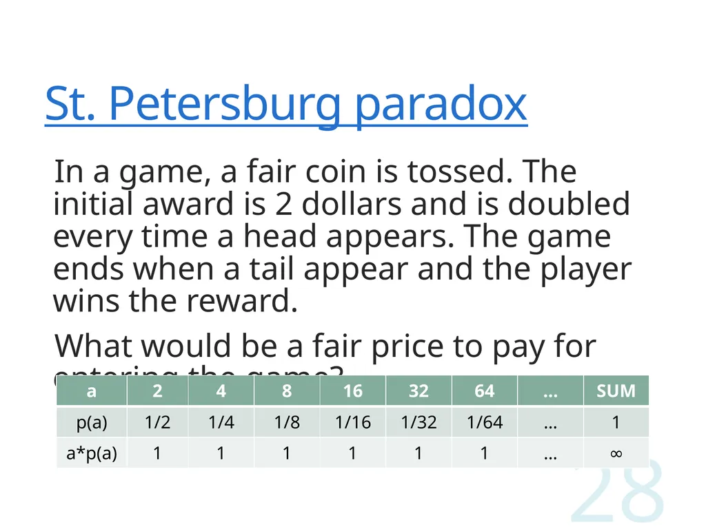
slide28. St. Petersburg paradox In a game, a fair coin is tossed. The initial award is 2 dollars and is doubled every time a head appears. The game ends when a tail appear and the player wins the reward.
What would be a fair price to pay for entering the game? 28<br>
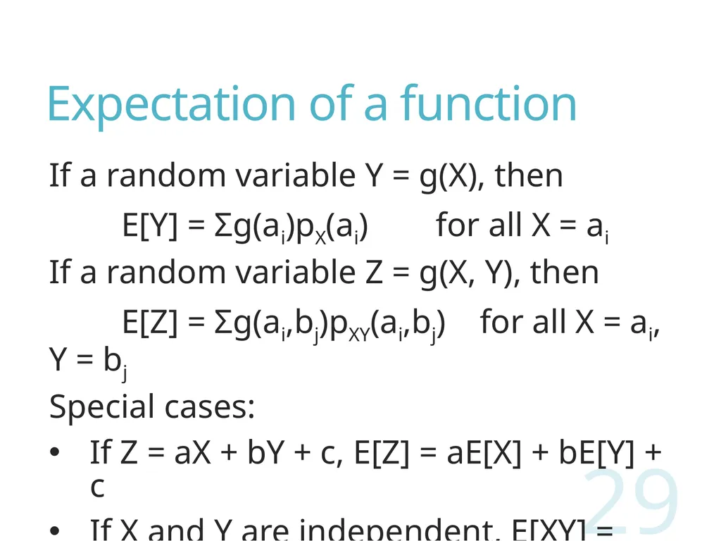
slide29. Expectation of a function If a random variable Y = g(X), then
E[Y] = Ʃg(ai)pX(ai) for all X = ai
If a random variable Z = g(X, Y), then
E[Z] = Ʃg(ai,bj)pXY(ai,bj) for all X = ai, Y = bj
Special cases:
If Z = aX + bY + c, E[Z] = aE[X] + bE[Y] + c
If X and Y are independent, E[XY] = E[X]E[Y] 29<br>
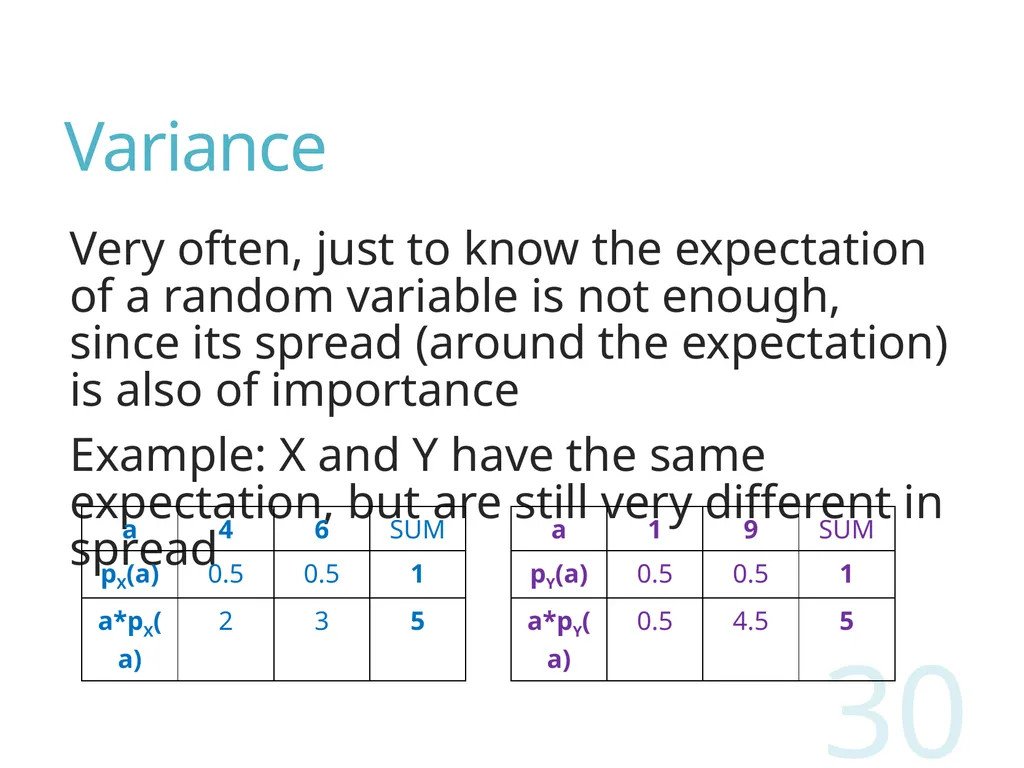
slide30. Variance Very often, just to know the expectation of a random variable is not enough, since its spread (around the expectation) is also of importance
Example: X and Y have the same expectation, but are still very different in spread 30<br>
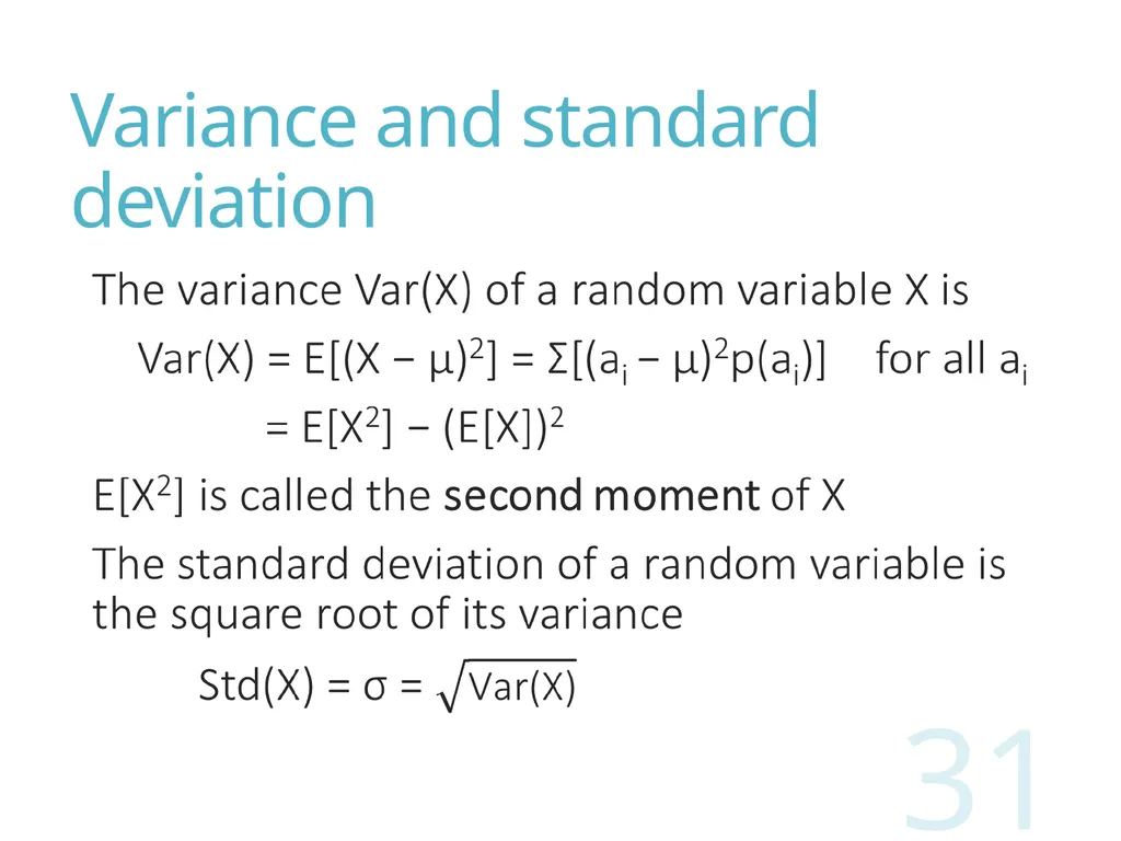
slide31. Variance and standard deviation 31<br>
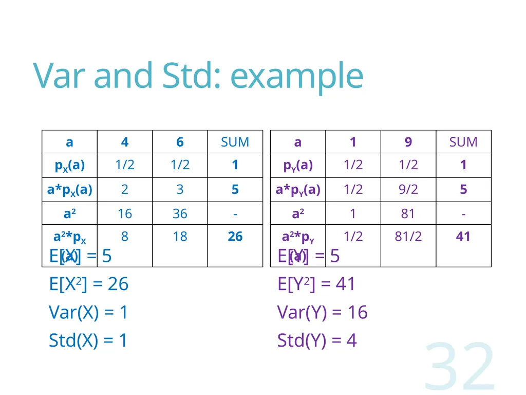
slide32. Var and Std: example 32 E[X] = 5
E[X2] = 26
Var(X) = 1
Std(X) = 1 E[Y] = 5
E[Y2] = 41
Var(Y) = 16
Std(Y) = 4<br>
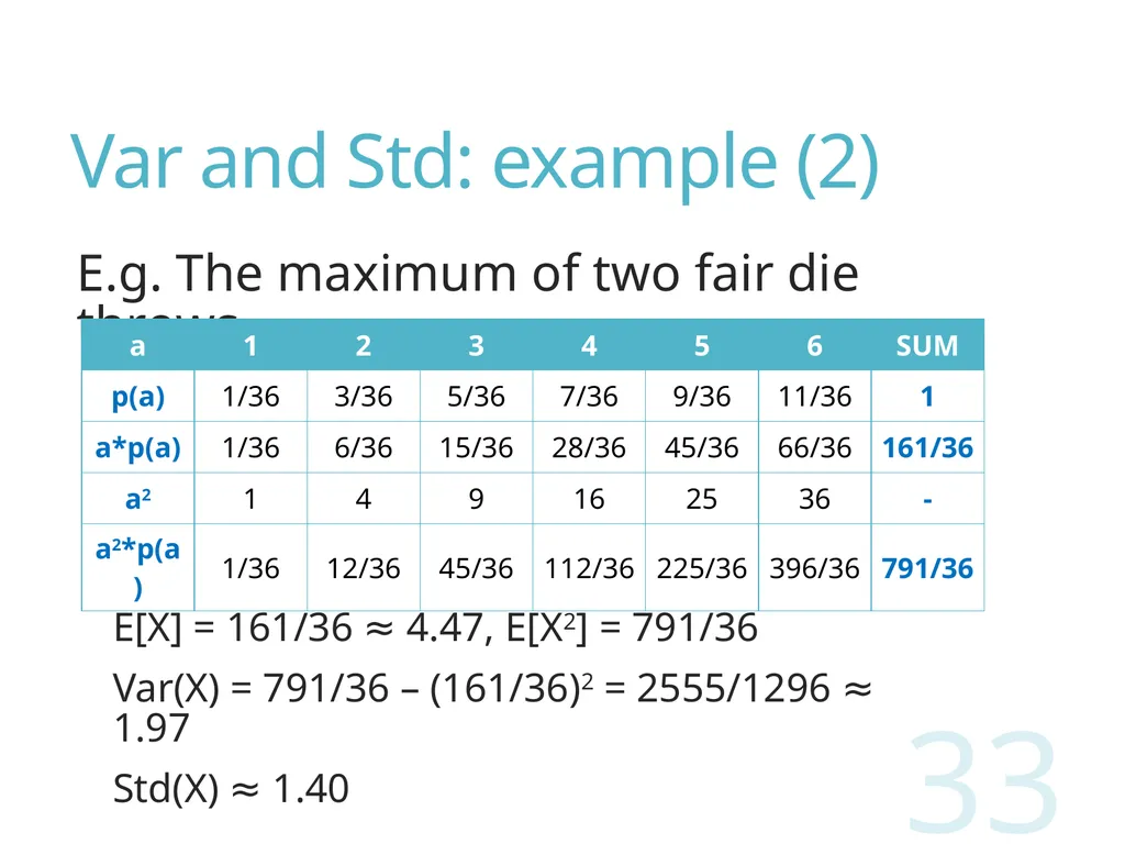
slide33. Var and Std: example (2) E.g. The maximum of two fair die throws 33 E[X] = 161/36 ≈ 4.47, E[X2] = 791/36
Var(X) = 791/36 – (161/36)2 = 2555/1296 ≈ 1.97
Std(X) ≈ 1.40<br>
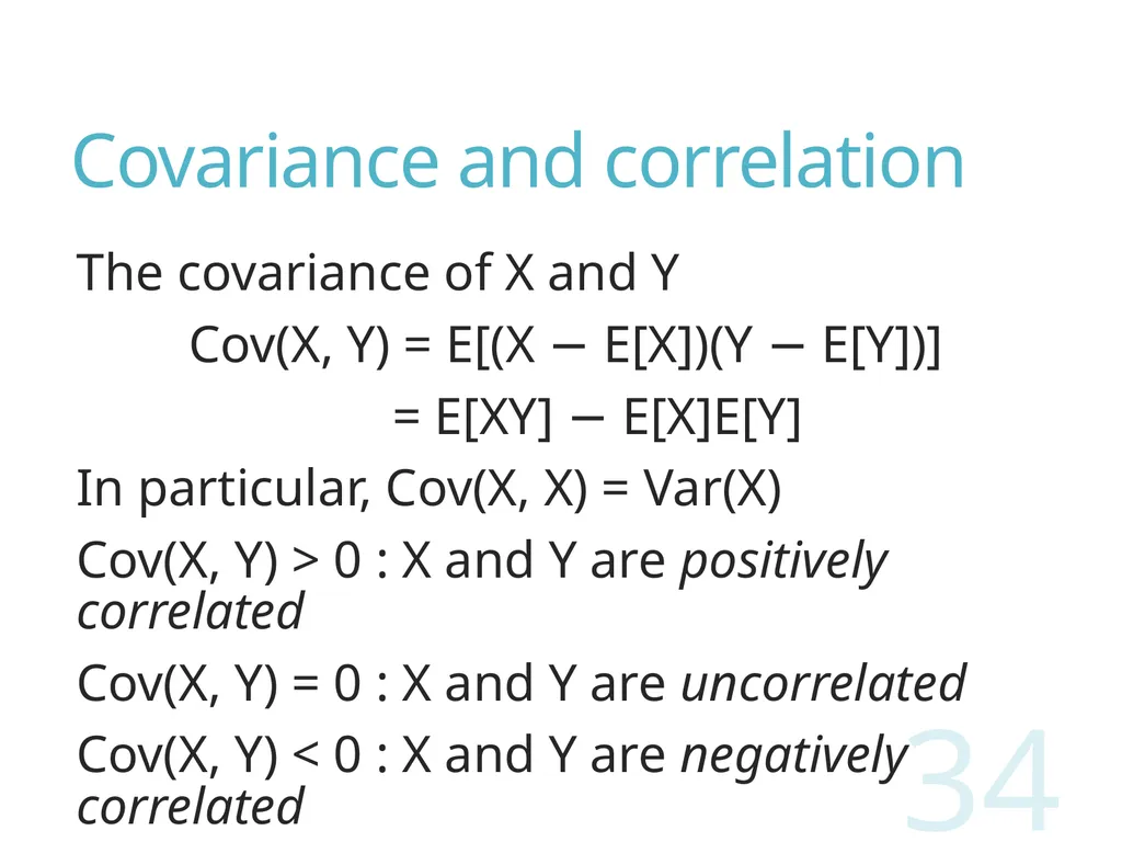
slide34. Covariance and correlation The covariance of X and Y
Cov(X, Y) = E[(X − E[X])(Y − E[Y])]
= E[XY] − E[X]E[Y]
In particular, Cov(X, X) = Var(X)
Cov(X, Y) > 0 : X and Y are positively correlated
Cov(X, Y) = 0 : X and Y are uncorrelated
Cov(X, Y) < 0 : X and Y are negatively correlated 34<br>
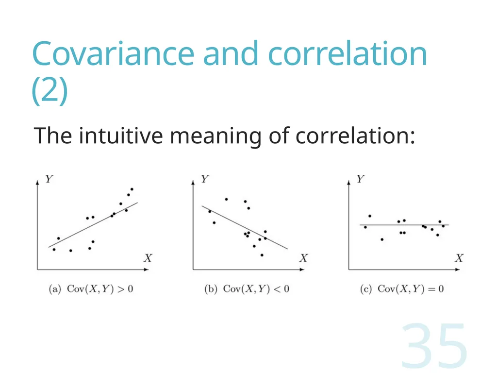
slide35. Covariance and correlation (2) The intuitive meaning of correlation: 35<br>
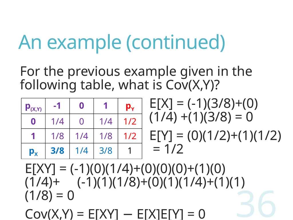
slide36. An example (continued) For the previous example given in the following table, what is Cov(X,Y)? 36 E[XY] = (-1)(0)(1/4)+(0)(0)(0)+(1)(0)(1/4)+ (-1)(1)(1/8)+(0)(1)(1/4)+(1)(1)(1/8) = 0
Cov(X,Y) = E[XY] − E[X]E[Y] = 0 E[X] = (-1)(3/8)+(0)(1/4) +(1)(3/8) = 0
E[Y] = (0)(1/2)+(1)(1/2) = 1/2<br>
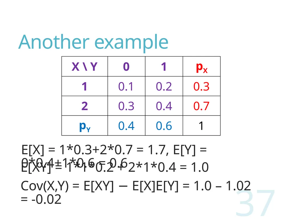
slide37. Another example 37 E[X] = 1*0.3+2*0.7 = 1.7, E[Y] = 0*0.4+1*0.6 = 0.6 E[XY] = 1*1*0.2 + 2*1*0.4 = 1.0
Cov(X,Y) = E[XY] − E[X]E[Y] = 1.0 – 1.02 = -0.02<br>
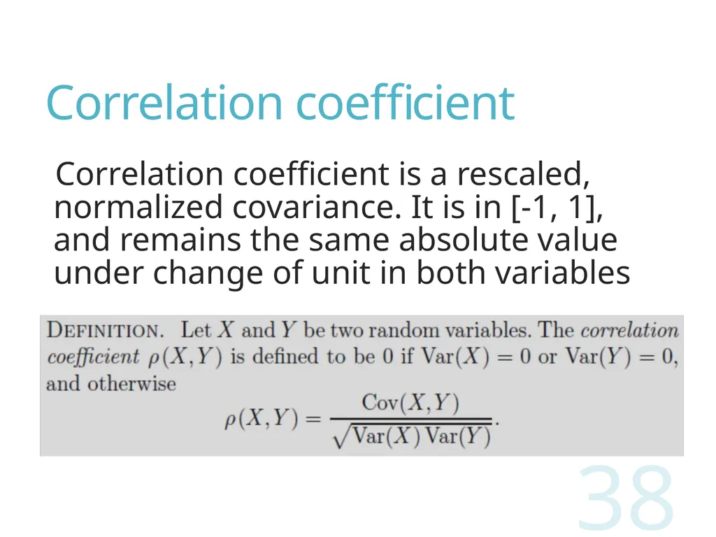
slide38. Correlation coefficient Correlation coefficient is a rescaled, normalized covariance. It is in [-1, 1], and remains the same absolute value under change of unit in both variables 38<br>
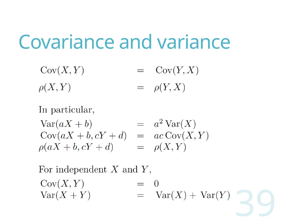
slide39. Covariance and variance 39<br>
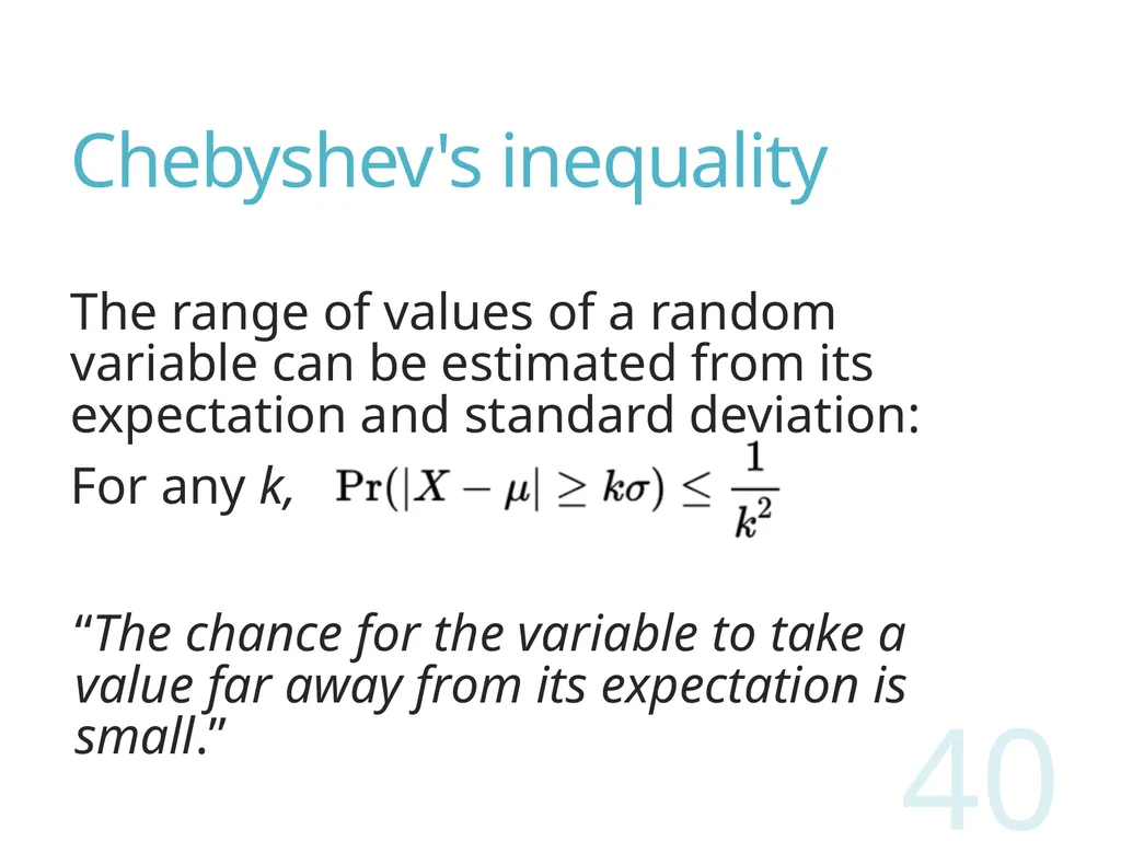
slide40. Chebyshev's inequality The range of values of a random variable can be estimated from its expectation and standard deviation:
For any k, 40 “The chance for the variable to take a value far away from its expectation is small.”<br>
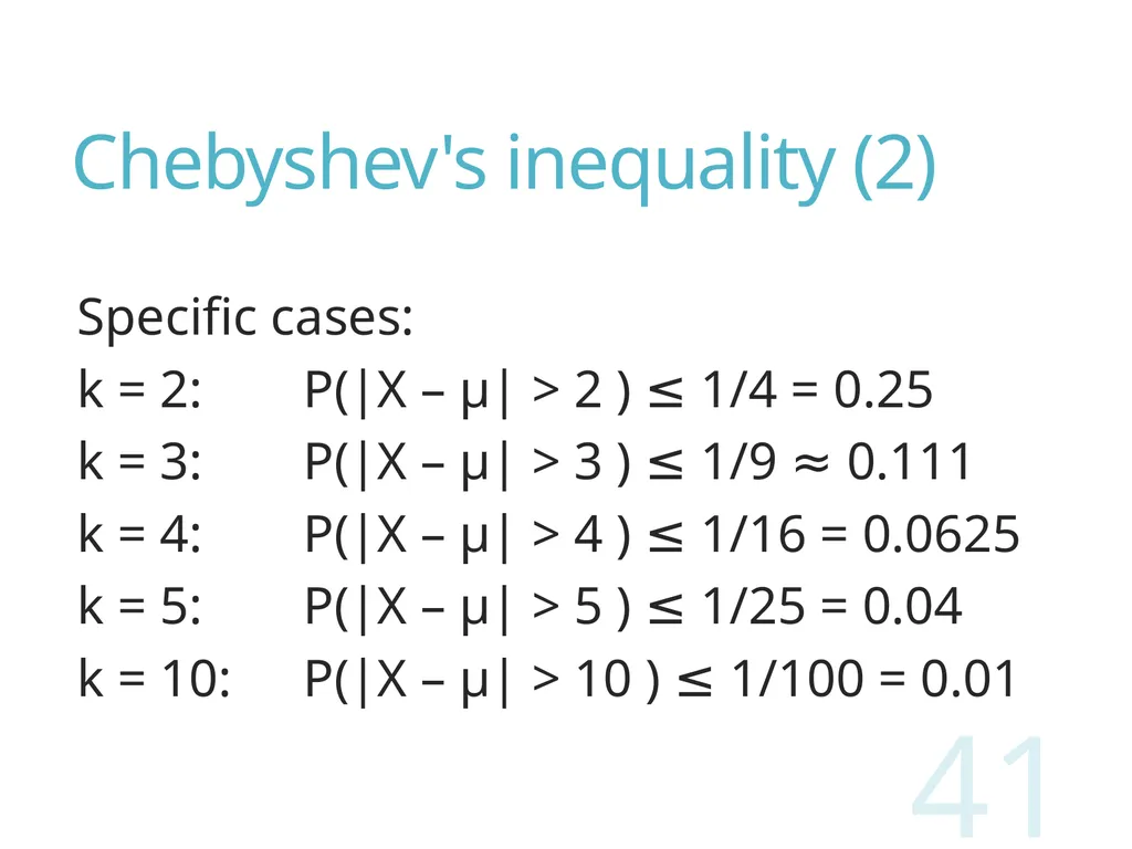
slide41. Chebyshev's inequality (2) Specific cases:
k = 2: P(|X – μ| > 2) ≤ 1/4 = 0.25
k = 3: P(|X – μ| > 3) ≤ 1/9 ≈ 0.111
k = 4: P(|X – μ| > 4) ≤ 1/16 = 0.0625
k = 5: P(|X – μ| > 5) ≤ 1/25 = 0.04
k = 10: P(|X – μ| > 10) ≤ 1/100 = 0.01 41<br>
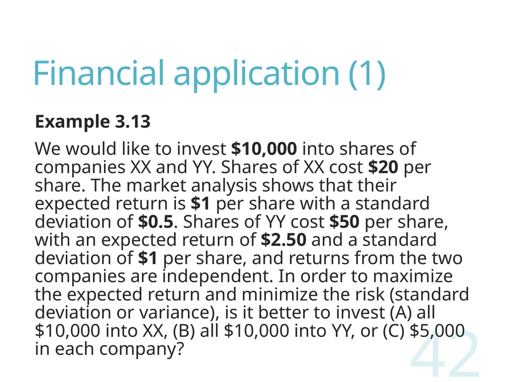
slide42. Financial application (1) Example 3.13
We would like to invest $10,000 into shares of companies XX and YY. Shares of XX cost $20 per share. The market analysis shows that their expected return is $1 per share with a standard deviation of $0.5. Shares of YY cost $50 per share, with an expected return of $2.50 and a standard deviation of $1 per share, and returns from the two companies are independent. In order to maximize the expected return and minimize the risk (standard deviation or variance), is it better to invest (A) all $10,000 into XX, (B) all $10,000 into YY, or (C) $5,000 in each company? 42<br>
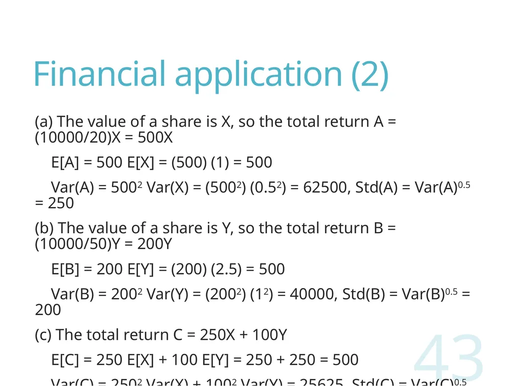
slide43. Financial application (2) (a) The value of a share is X, so the total return A = (10000/20)X = 500X
E[A] = 500 E[X] = (500) (1) = 500
Var(A) = 5002 Var(X) = (5002) (0.52) = 62500, Std(A) = Var(A)0.5 = 250
(b) The value of a share is Y, so the total return B = (10000/50)Y = 200Y
E[B] = 200 E[Y] = (200) (2.5) = 500
Var(B) = 2002 Var(Y) = (2002) (12) = 40000, Std(B) = Var(B)0.5 = 200
(c) The total return C = 250X + 100Y
E[C] = 250 E[X] + 100 E[Y] = 250 + 250 = 500
Var(C) = 2502 Var(X) + 1002 Var(Y) = 25625, Std(C) = Var(C)0.5 ≈ 160 43<br>
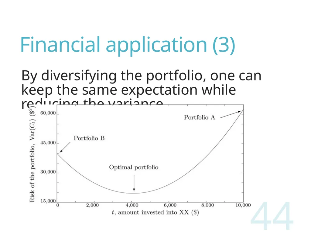
slide44. Financial application (3) By diversifying the portfolio, one can keep the same expectation while reducing the variance 44<br>
slide45. Bernoulli distribution A random variable with two possible values, 0 and 1, is called a Bernoulli variable, and its distribution is Bernoulli distribution
Ber(p) is a Bernoulli distribution with parameter p, where 0 ≤ p ≤ 1, and
p(1) = P(X = 1) = p
p(0) = P(X = 0) = 1 − p
E[X] = p, Var(X) = p(1 − p) 45<br>
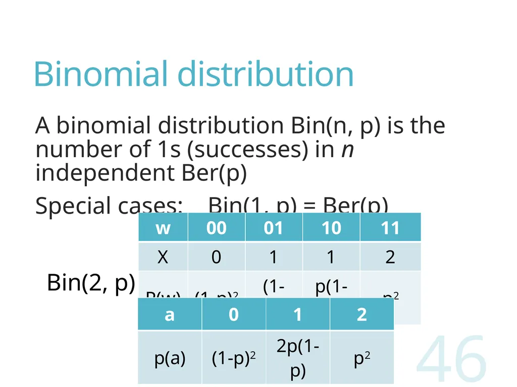
slide46. Binomial distribution A binomial distribution Bin(n, p) is the number of 1s (successes) in n independent Ber(p)
Special cases: Bin(1, p) = Ber(p) 46 Bin(2, p)<br>
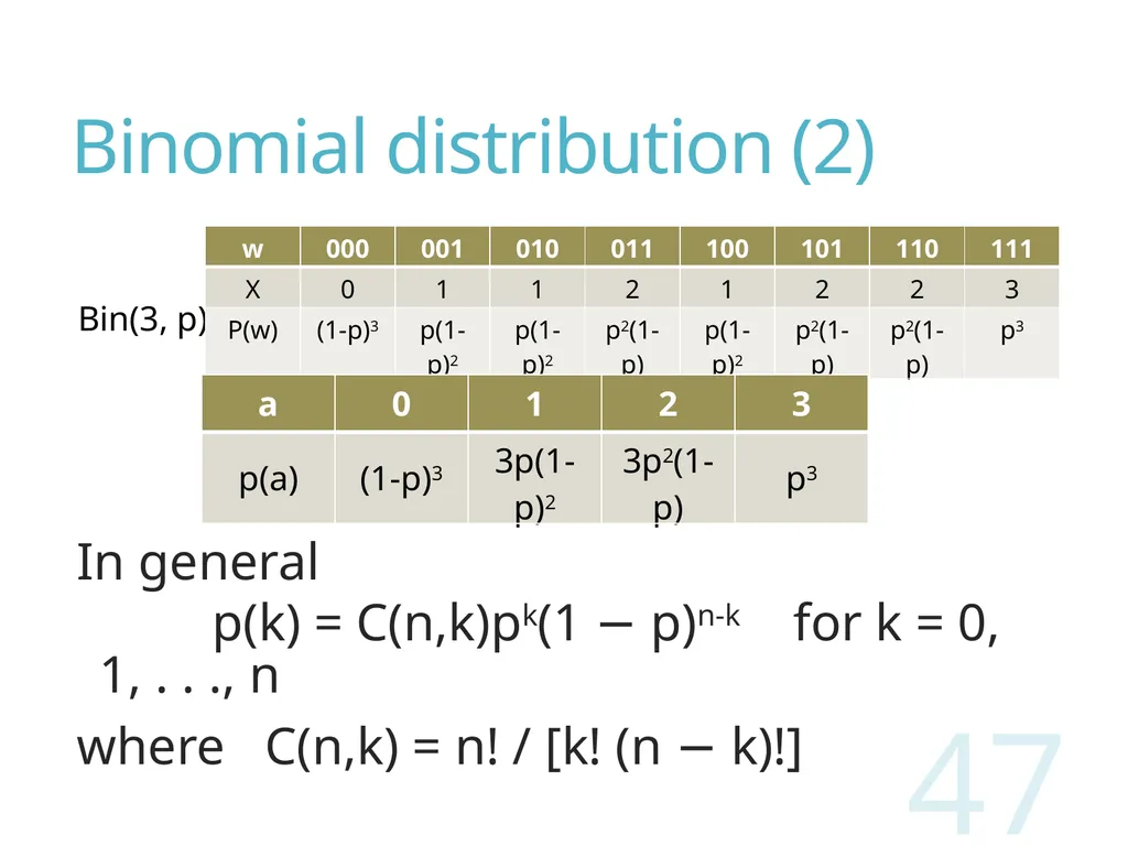
slide47. Binomial distribution (2) In general
p(k) = C(n,k)pk(1 − p)n-k for k = 0, 1, . . ., n
where C(n,k) = n! / [k! (n − k)!] 47 Bin(3, p)<br>
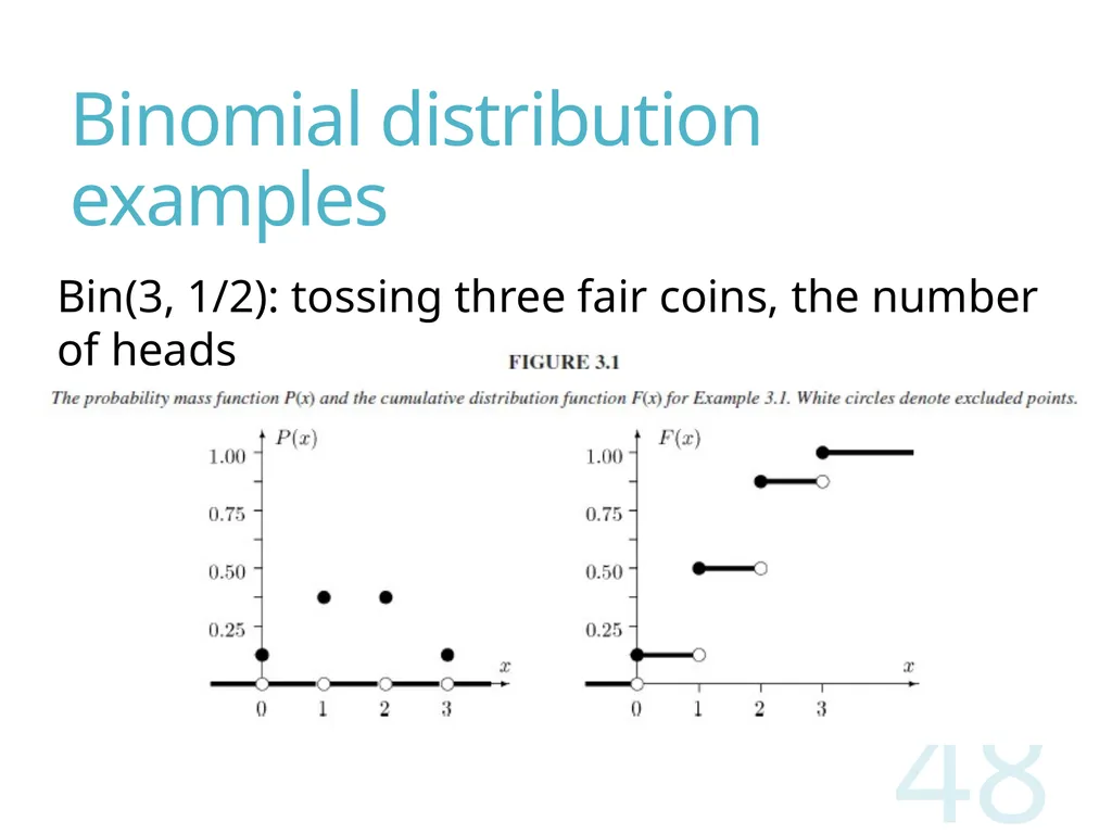
slide48. Binomial distribution examples 48 Bin(3, 1/2): tossing three fair coins, the number of heads<br>
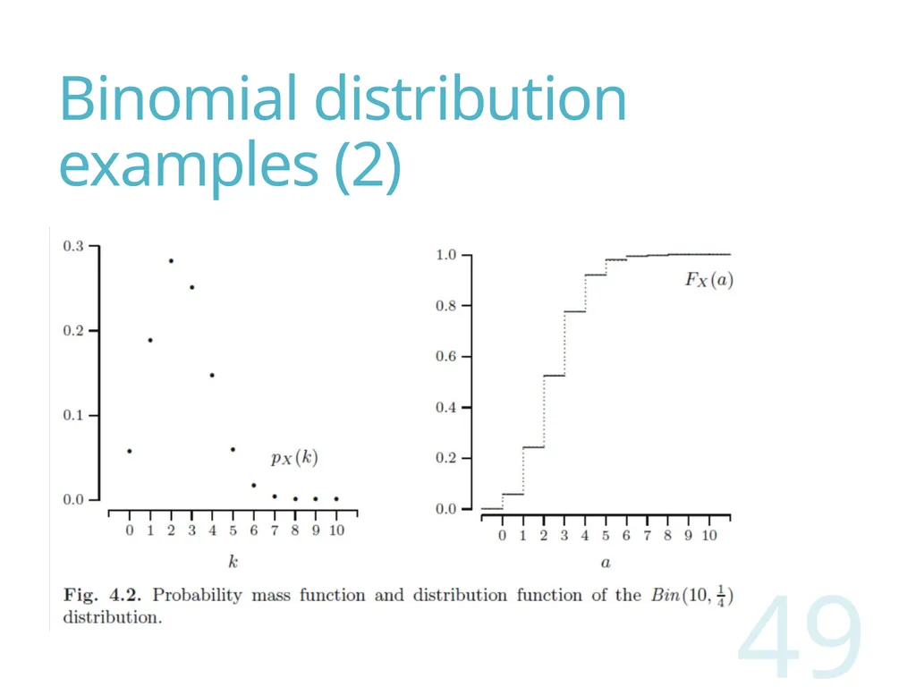
slide49. Binomial distribution examples (2) 49<br>
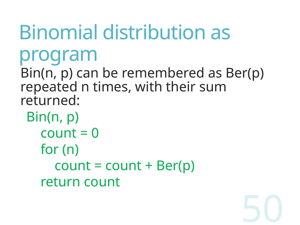
slide50. Binomial distribution as program Bin(n, p) can be remembered as Ber(p) repeated n times, with their sum returned:
Bin(n, p)
count = 0
for (n)
count = count + Ber(p)
return count 50<br>
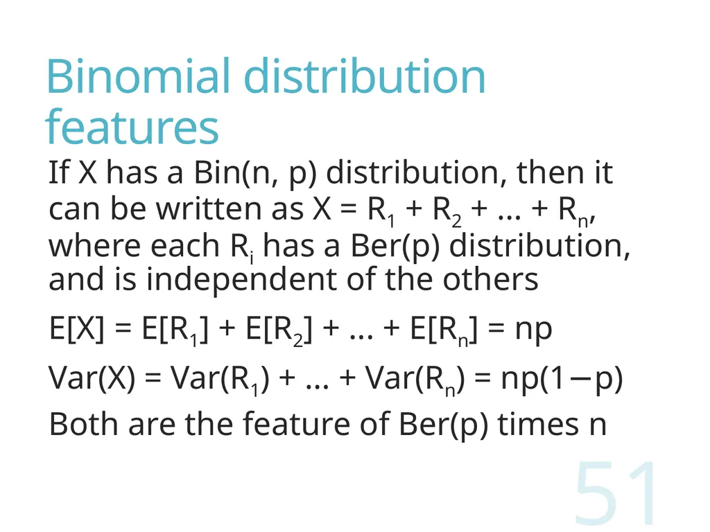
slide51. Binomial distribution features If X has a Bin(n, p) distribution, then it can be written as X = R1 + R2 + ... + Rn, where each Ri has a Ber(p) distribution, and is independent of the others
E[X] = E[R1] + E[R2] + ... + E[Rn] = np
Var(X) = Var(R1) + ... + Var(Rn) = np(1−p)
Both are the feature of Ber(p) times n 51<br>
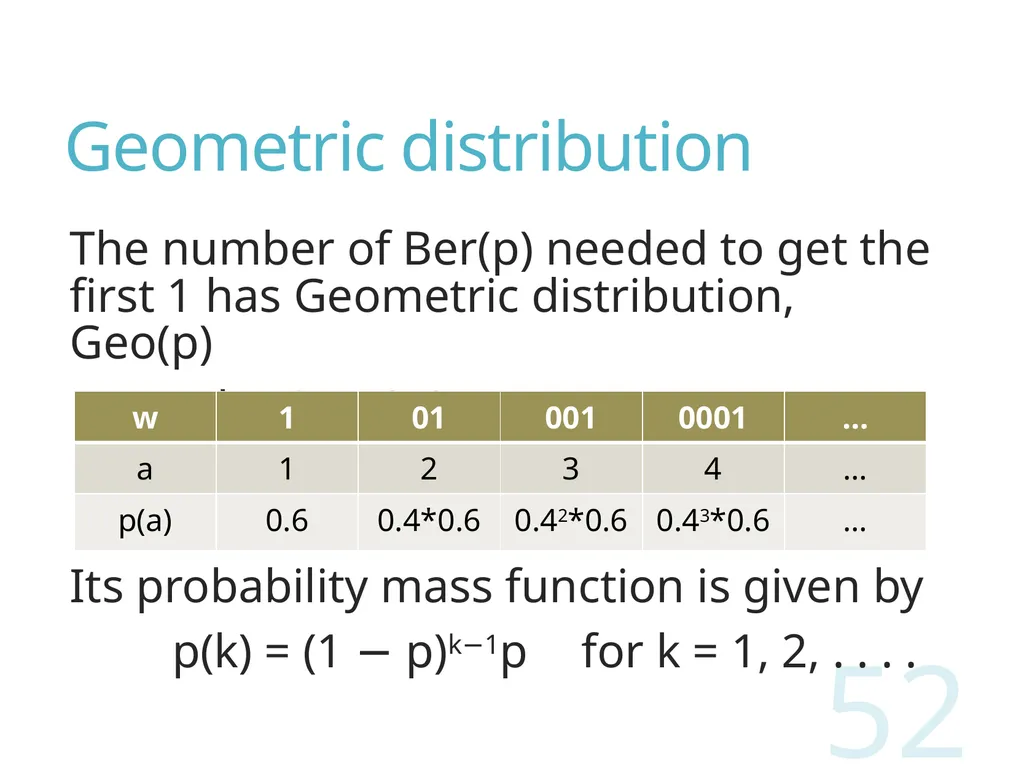
slide52. Geometric distribution The number of Ber(p) needed to get the first 1 has Geometric distribution, Geo(p)
Example: Geo(0.6) 52 Its probability mass function is given by
p(k) = (1 − p)k−1p for k = 1, 2, . . . .<br>
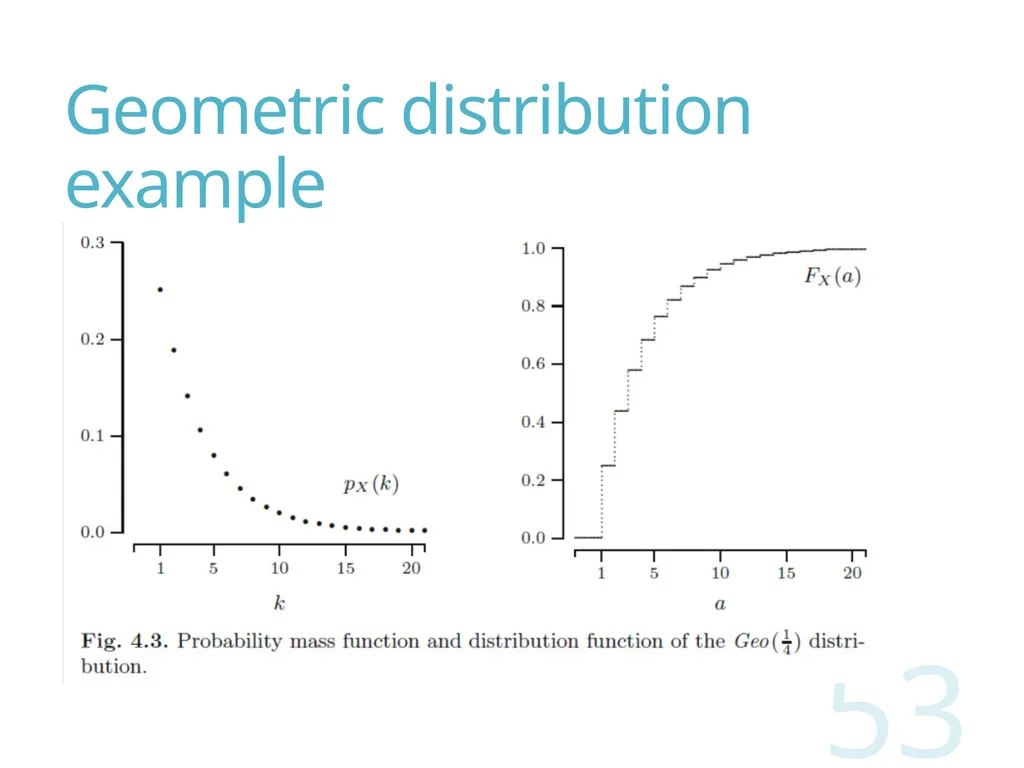
slide53. Geometric distribution example 53<br>
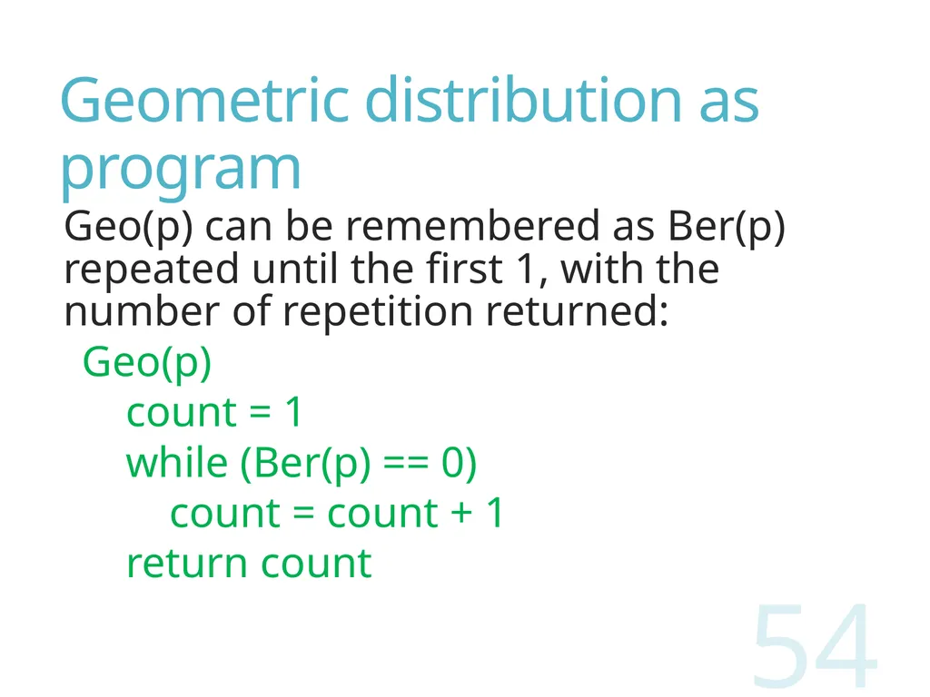
slide54. Geometric distribution as program Geo(p) can be remembered as Ber(p) repeated until the first 1, with the number of repetition returned:
Geo(p)
count = 1
while (Ber(p) == 0)
count = count + 1
return count 54<br>
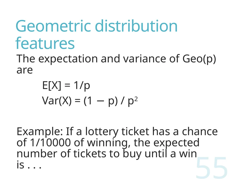
slide55. Geometric distribution features The expectation and variance of Geo(p) are
E[X] = 1/p
Var(X) = (1 − p) / p2

Example: If a lottery ticket has a chance of 1/10000 of winning, the expected number of tickets to buy until a win is . . . 55<br>
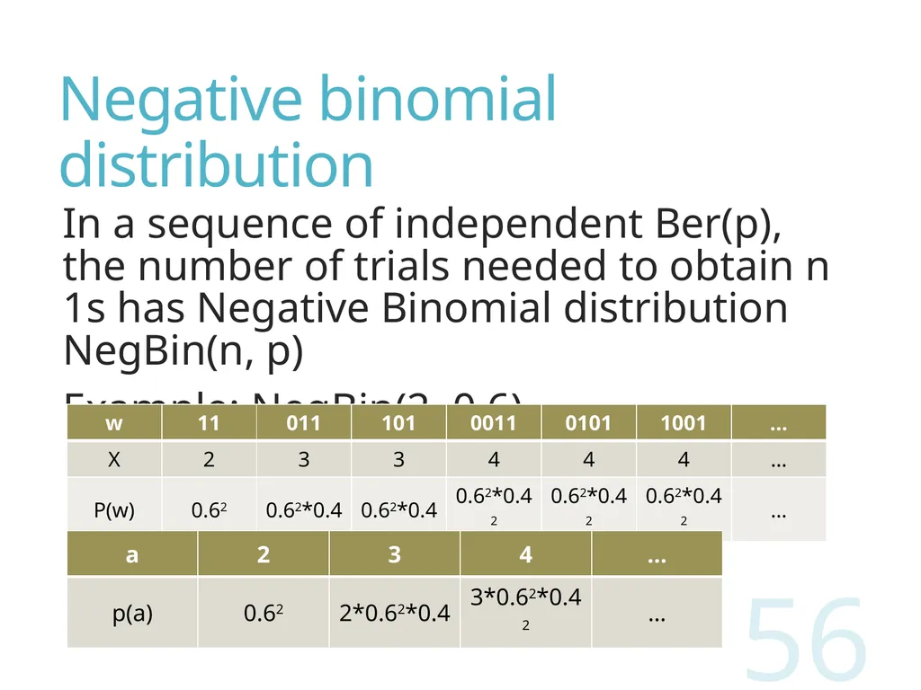
slide56. Negative binomial distribution In a sequence of independent Ber(p), the number of trials needed to obtain n 1s has Negative Binomial distribution NegBin(n, p)
Example: NegBin(2, 0.6) 56<br>
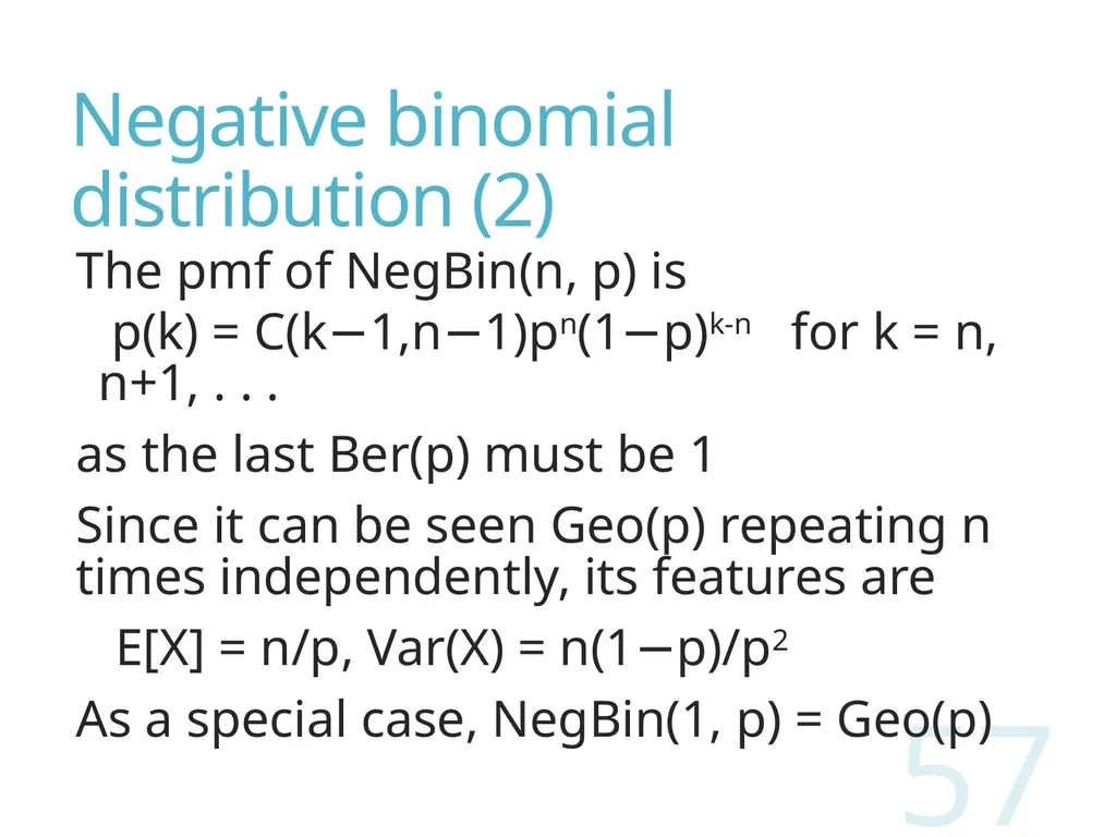
slide57. Negative binomial distribution (2) The pmf of NegBin(n, p) is
p(k) = C(k−1,n−1)pn(1−p)k-n for k = n, n+1, . . .
as the last Ber(p) must be 1
Since it can be seen Geo(p) repeating n times independently, its features are
E[X] = n/p, Var(X) = n(1−p)/p2
As a special case, NegBin(1, p) = Geo(p) 57<br>
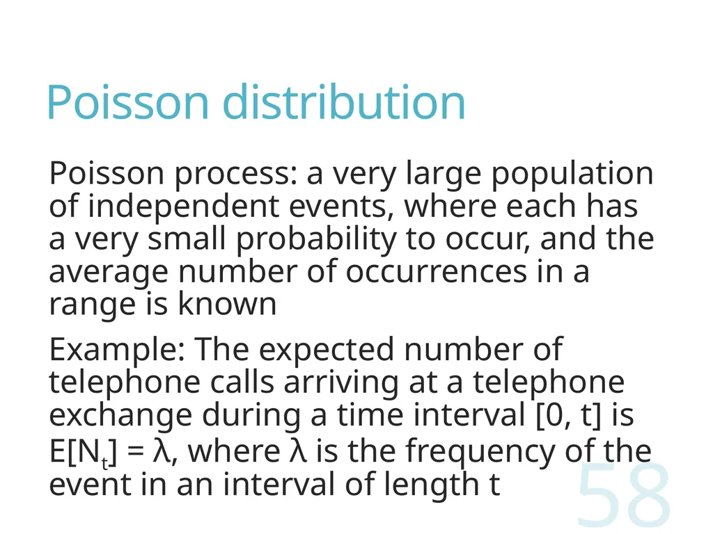
slide58. Poisson distribution Poisson process: a very large population of independent events, where each has a very small probability to occur, and the average number of occurrences in a range is known
Example: The expected number of telephone calls arriving at a telephone exchange during a time interval [0, t] is E[Nt] = λ, where λ is the frequency of the event in an interval of length t 58<br>
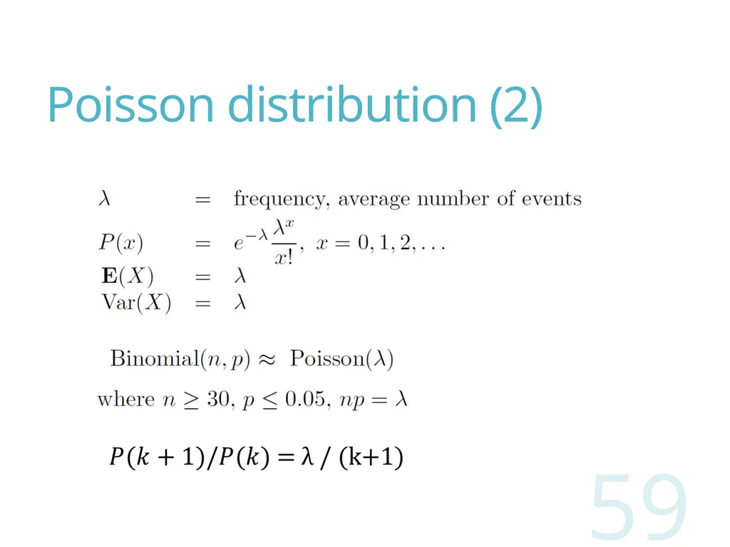
slide59. Poisson distribution (2) 59<br>
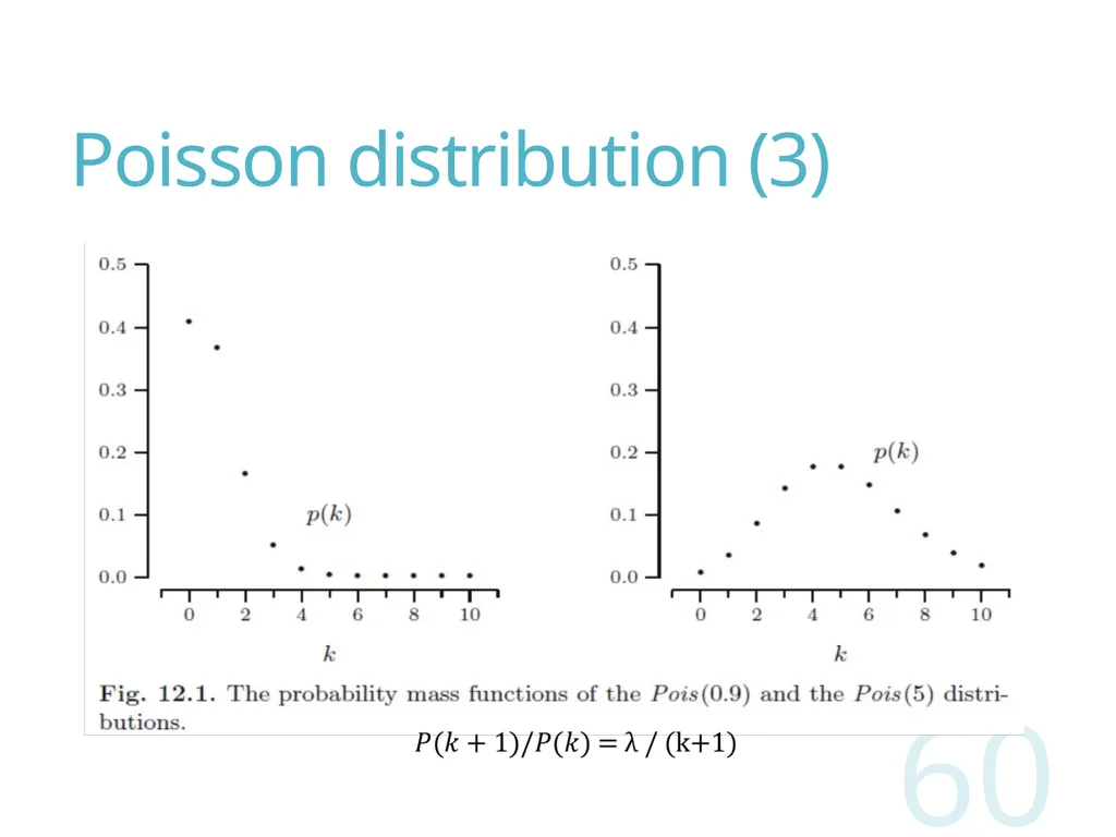
slide60. Poisson distribution (3) 60<br>
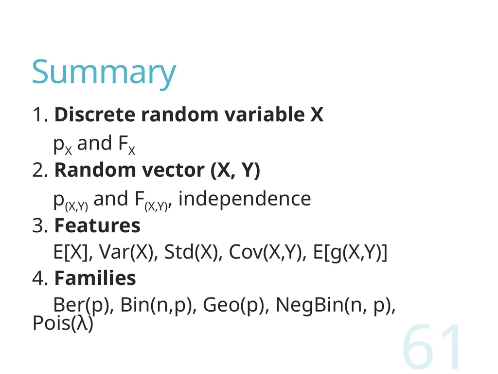
slide61. Summary 1. Discrete random variable X
pX and FX
2. Random vector (X, Y)
p(X,Y) and F(X,Y), independence
3. Features
E[X], Var(X), Std(X), Cov(X,Y), E[g(X,Y)]
4. Families
Ber(p), Bin(n,p), Geo(p), NegBin(n, p), Pois(λ) 61<br>
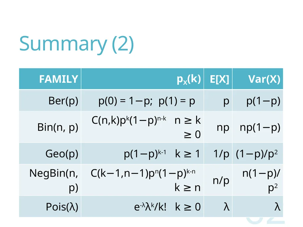
slide62. Summary (2) 62<br>