
Psychology 105 Advanced Research Methods February

Description: Psychology 105 Advanced Research Methods February 9, 2021 New concept: random variables Review definition of variables and distributions New kind of variable: imaginary a set of values that could occur random variable Distribution of a
Related Topics
Download Presentation
"Psychology 105 Advanced Research Methods February" is the property of its rightful owner. Permission is granted to download and print the materials on this website for personal, non-commercial use only, and to display it on your personal computer provided you do not modify the materials and that you retain all copyright notices contained in the materials. By downloading content from our website, you accept the terms of this agreement.
Presentation Transcript
slide1. Psychology 105
Advanced Research Methods February 9, 2021<br>
slide2. New concept: random variables Review definition of variables and distributions
New kind of variable:
imaginary
a set of values that could occur
random variable<br>
slide3. Distribution of a random variable Just as variables have distributions, so do random variables.
The distribution of a random variable is the set of values that could occur if we were to observe the variable…
…together with the long run relative frequencies with which those values would occur.<br>
slide4. Probability distributions This special type of imaginary distribution is called a probability distribution.
Definition: A probability distribution is the set of values that could occur for a random variable, together with the long-run relative frequencies with which they do occur when that random variable is actually observed.<br>
slide5. Frequentist approach long-run relative frequency = probability
The law of large numbers:
If a random process is observed repeatedly, the proportion of times a particular outcome of that process occurs approaches the probability of the outcome as the number of repetitions becomes large.<br>
slide6. More detail on the frequentist approach Just as relative frequency observed in the long run is probability...
...descriptive statistics observed in the long run become parameters of the probability distribution,
...and graphics observed in the long run become pictures of the probability distribution.<br>
slide7. Some technical matters A well-defined outcome of a random variable is called an event.
Random variables may be continuous or discrete.
The probability of any particular outcome for a continuous random variable is zero.
In such cases, events must be described in terms of ranges of possible values.<br>
slide8. Bernoulli trials: the simplest possible random variable On each repetition, one of two discrete values may occur, and the probability of each is the same on each trial.
Examples:
tossing a coin
rolling a die
choosing a random person and observing that person’s sex<br>
slide9. Bernoulli processes The name for that type of random variable is Bernoulli random variable or Bernoulli process.
Think about the example of tossing a fair coin.
digression on virtual whiteboard and in R<br>
slide10. Recapping types of distributions So far, we have discussed two types of distributions
Distributions:
Values that a variable takes on, with frequencies (or relative frequencies) of those values
Probability distributions:
Values that a random variable could take on, together with probabilities of those values<br>
slide11. Similarities We’ve seen that the same ways of thinking can help us understand the shape of both types of distribution.
The trick to understanding probability distributions is to apply those ways of thinking to what would happen in the long run.<br>
slide12. Continuous random variables Examples:
Normal distribution
Uniform distribution
New terminology: probability density function (abbreviated “pdf”)
Investigating some properties of the uniform distribution<br>
slide13. The addition rule Used for combining events with an “OR” link.
Simple form (requires mutually exclusive events): P(A or B) = P(A) + P(B)
Examples:
P(a die comes up 1 OR 2)
P(spinner lands between 0 and ¼ OR between ½ and ¾)
P( N(0,1) < -1.96 OR > 1.96)<br>
slide14. The addition rule (cont.) The more complex form: P(A or B) = P(A) + P(B) – P(A and B).
Does not require mutual exclusivity.
Examples:
P( 1st coin toss is 'H' OR 2nd coin toss is 'H')
P( 1st IQ > 136 OR 2nd IQ > 136)
But there's a problem: how do we get P(A and B)?<br>
slide15. The multiplication rule Used for combining events with an 'AND' link.
Simple form (requires independent events): P(A and B) = P(A) P(B).
Examples:
P( 1st coin toss = 'H' AND 2nd coin toss = 'H')
P( 1st spin > ½ AND 2nd spin < ¾ )<br>
slide16. The multiplication rule (cont.) The more complex form (does not require independence):
P(A and B) = P(A) P(B|A) or
P(A and B) = P(B) P(A|B)
The vertical bar is read “given” and indicates conditional probability.<br>
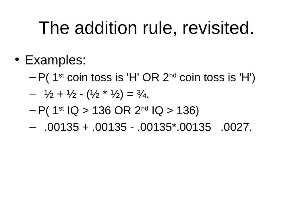
slide17. The addition rule, revisited. Examples:
P( 1st coin toss is 'H' OR 2nd coin toss is 'H')
½ + ½ - (½ * ½) = ¾.
P( 1st IQ > 136 OR 2nd IQ > 136)
.00135 + .00135 - .00135*.00135 .0027.<br>
slide18. Empirical validation of probability laws An interlude in R occurs here.<br>
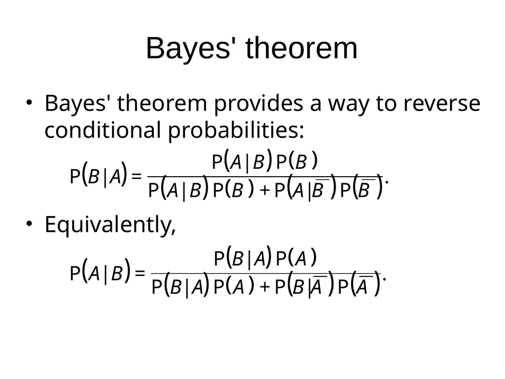
slide19. Bayes' theorem Bayes' theorem provides a way to reverse conditional probabilities:
Equivalently,<br>
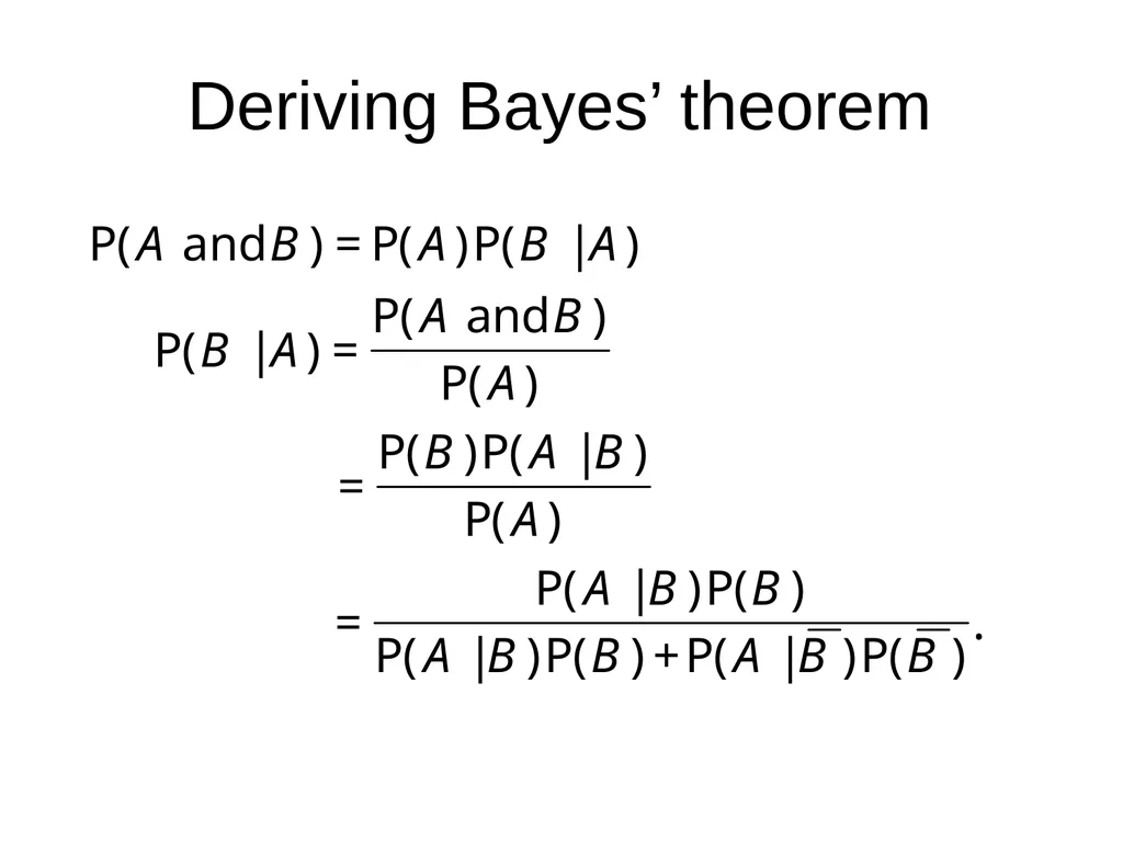
slide20. Deriving Bayes’ theorem<br>
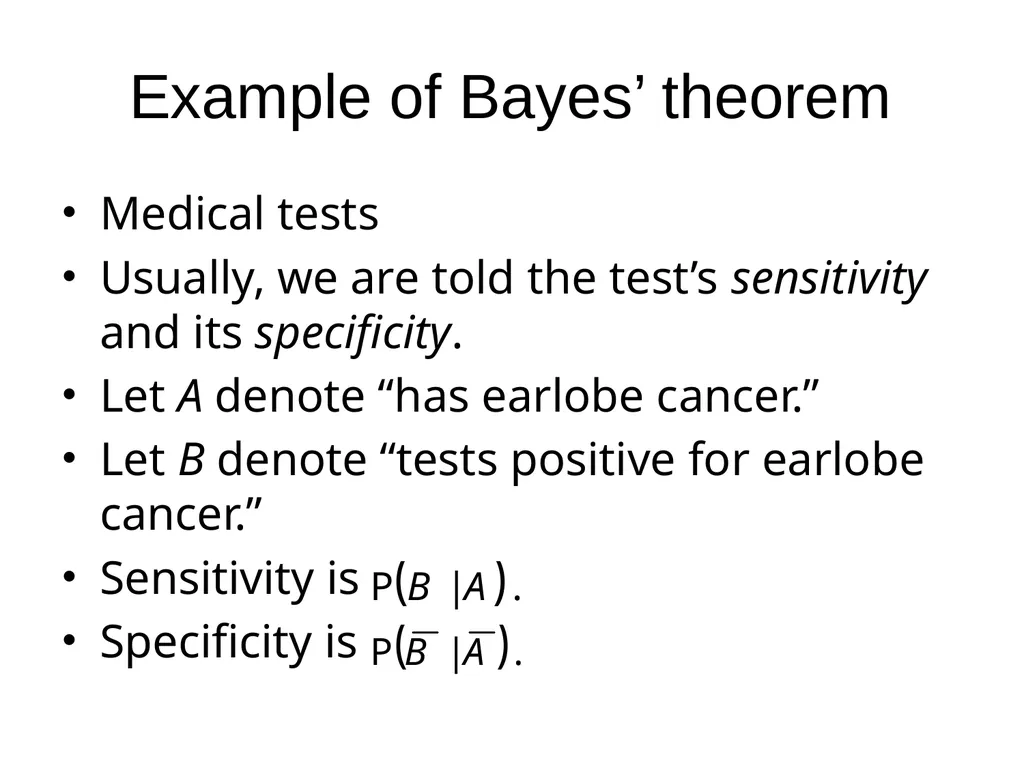
slide21. Example of Bayes’ theorem Medical tests
Usually, we are told the test’s sensitivity and its specificity.
Let A denote “has earlobe cancer.”
Let B denote “tests positive for earlobe cancer.”
Sensitivity is
Specificity is<br>
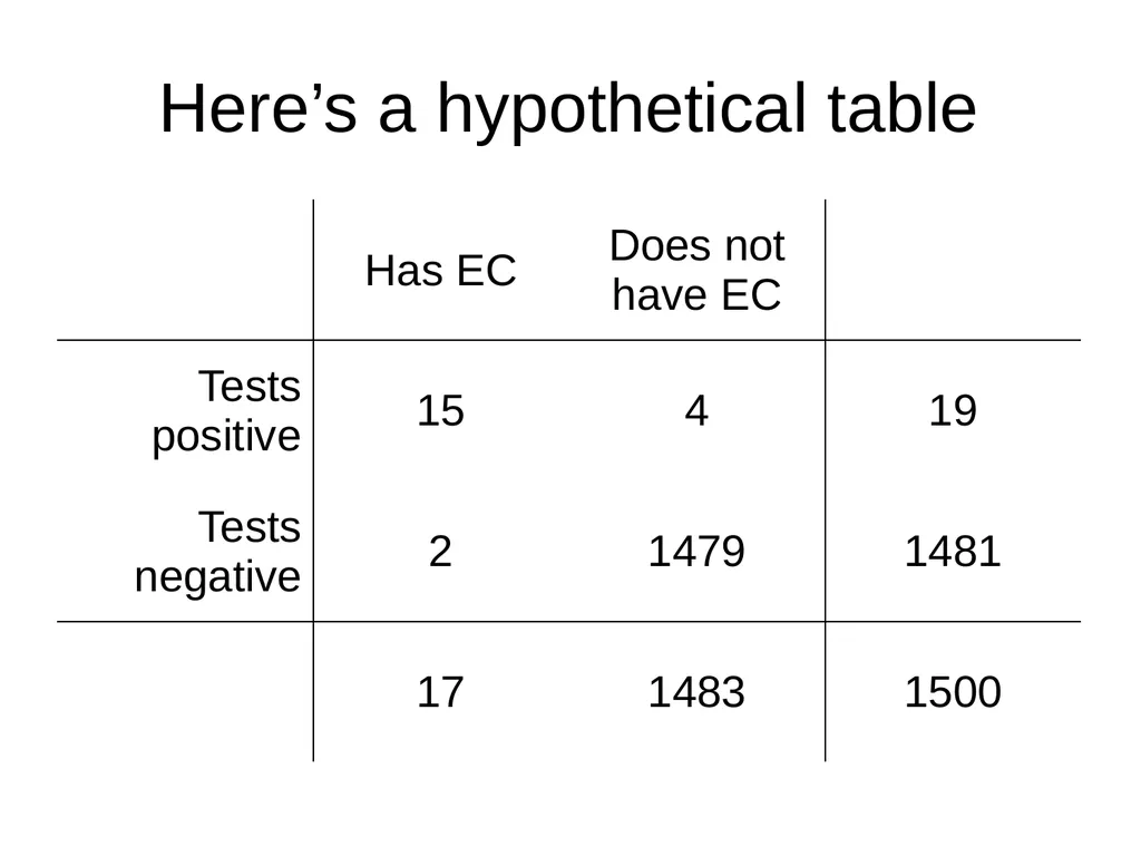
slide22. Here’s a hypothetical table<br>
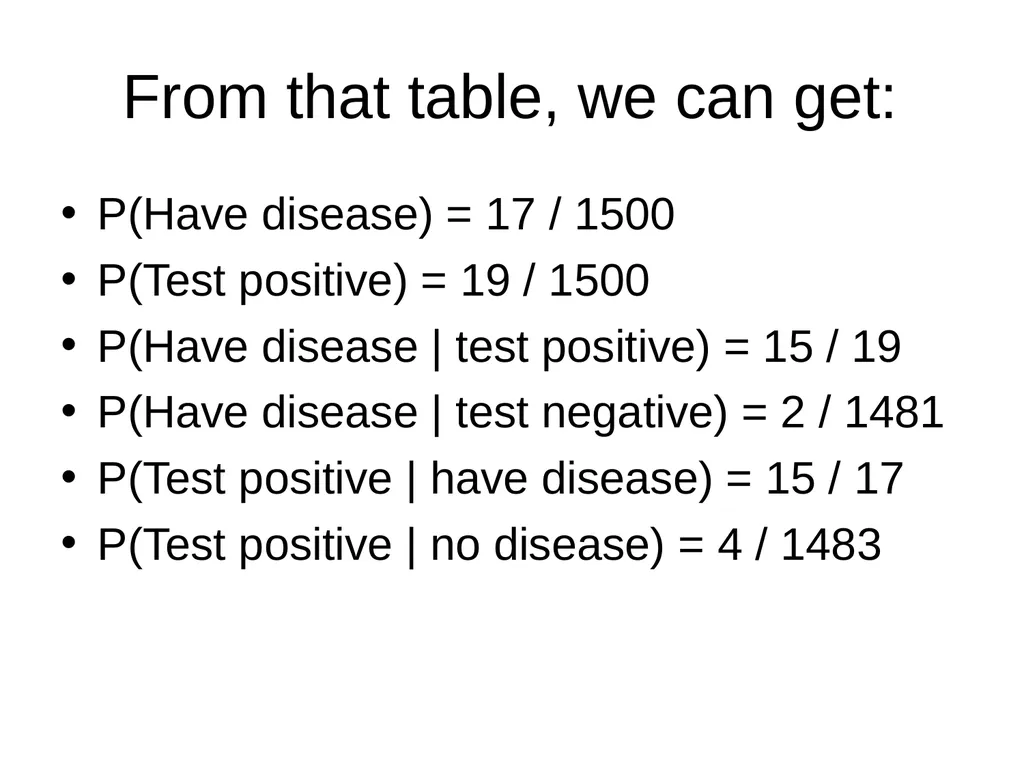
slide23. From that table, we can get: P(Have disease) = 17 / 1500
P(Test positive) = 19 / 1500
P(Have disease | test positive) = 15 / 19
P(Have disease | test negative) = 2 / 1481
P(Test positive | have disease) = 15 / 17
P(Test positive | no disease) = 4 / 1483<br>
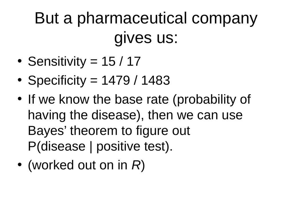
slide24. But a pharmaceutical company gives us: Sensitivity = 15 / 17
Specificity = 1479 / 1483
If we know the base rate (probability of having the disease), then we can use Bayes’ theorem to figure out P(disease | positive test).
(worked out on in R)<br>
slide2. New concept: random variables Review definition of variables and distributions
New kind of variable:
imaginary
a set of values that could occur
random variable<br>
slide3. Distribution of a random variable Just as variables have distributions, so do random variables.
The distribution of a random variable is the set of values that could occur if we were to observe the variable…
…together with the long run relative frequencies with which those values would occur.<br>
slide4. Probability distributions This special type of imaginary distribution is called a probability distribution.
Definition: A probability distribution is the set of values that could occur for a random variable, together with the long-run relative frequencies with which they do occur when that random variable is actually observed.<br>
slide5. Frequentist approach long-run relative frequency = probability
The law of large numbers:
If a random process is observed repeatedly, the proportion of times a particular outcome of that process occurs approaches the probability of the outcome as the number of repetitions becomes large.<br>
slide6. More detail on the frequentist approach Just as relative frequency observed in the long run is probability...
...descriptive statistics observed in the long run become parameters of the probability distribution,
...and graphics observed in the long run become pictures of the probability distribution.<br>
slide7. Some technical matters A well-defined outcome of a random variable is called an event.
Random variables may be continuous or discrete.
The probability of any particular outcome for a continuous random variable is zero.
In such cases, events must be described in terms of ranges of possible values.<br>
slide8. Bernoulli trials: the simplest possible random variable On each repetition, one of two discrete values may occur, and the probability of each is the same on each trial.
Examples:
tossing a coin
rolling a die
choosing a random person and observing that person’s sex<br>
slide9. Bernoulli processes The name for that type of random variable is Bernoulli random variable or Bernoulli process.
Think about the example of tossing a fair coin.
digression on virtual whiteboard and in R<br>
slide10. Recapping types of distributions So far, we have discussed two types of distributions
Distributions:
Values that a variable takes on, with frequencies (or relative frequencies) of those values
Probability distributions:
Values that a random variable could take on, together with probabilities of those values<br>
slide11. Similarities We’ve seen that the same ways of thinking can help us understand the shape of both types of distribution.
The trick to understanding probability distributions is to apply those ways of thinking to what would happen in the long run.<br>
slide12. Continuous random variables Examples:
Normal distribution
Uniform distribution
New terminology: probability density function (abbreviated “pdf”)
Investigating some properties of the uniform distribution<br>
slide13. The addition rule Used for combining events with an “OR” link.
Simple form (requires mutually exclusive events): P(A or B) = P(A) + P(B)
Examples:
P(a die comes up 1 OR 2)
P(spinner lands between 0 and ¼ OR between ½ and ¾)
P( N(0,1) < -1.96 OR > 1.96)<br>
slide14. The addition rule (cont.) The more complex form: P(A or B) = P(A) + P(B) – P(A and B).
Does not require mutual exclusivity.
Examples:
P( 1st coin toss is 'H' OR 2nd coin toss is 'H')
P( 1st IQ > 136 OR 2nd IQ > 136)
But there's a problem: how do we get P(A and B)?<br>
slide15. The multiplication rule Used for combining events with an 'AND' link.
Simple form (requires independent events): P(A and B) = P(A) P(B).
Examples:
P( 1st coin toss = 'H' AND 2nd coin toss = 'H')
P( 1st spin > ½ AND 2nd spin < ¾ )<br>
slide16. The multiplication rule (cont.) The more complex form (does not require independence):
P(A and B) = P(A) P(B|A) or
P(A and B) = P(B) P(A|B)
The vertical bar is read “given” and indicates conditional probability.<br>
slide17. The addition rule, revisited. Examples:
P( 1st coin toss is 'H' OR 2nd coin toss is 'H')
½ + ½ - (½ * ½) = ¾.
P( 1st IQ > 136 OR 2nd IQ > 136)
.00135 + .00135 - .00135*.00135 .0027.<br>
slide18. Empirical validation of probability laws An interlude in R occurs here.<br>
slide19. Bayes' theorem Bayes' theorem provides a way to reverse conditional probabilities:
Equivalently,<br>
slide20. Deriving Bayes’ theorem<br>
slide21. Example of Bayes’ theorem Medical tests
Usually, we are told the test’s sensitivity and its specificity.
Let A denote “has earlobe cancer.”
Let B denote “tests positive for earlobe cancer.”
Sensitivity is
Specificity is<br>
slide22. Here’s a hypothetical table<br>
slide23. From that table, we can get: P(Have disease) = 17 / 1500
P(Test positive) = 19 / 1500
P(Have disease | test positive) = 15 / 19
P(Have disease | test negative) = 2 / 1481
P(Test positive | have disease) = 15 / 17
P(Test positive | no disease) = 4 / 1483<br>
slide24. But a pharmaceutical company gives us: Sensitivity = 15 / 17
Specificity = 1479 / 1483
If we know the base rate (probability of having the disease), then we can use Bayes’ theorem to figure out P(disease | positive test).
(worked out on in R)<br>