R Learning Module 1 GH 811 Lab: Week 1 January

lois-ondreau

Published 2026-08-12 · 26 slides · 0 views

↓ Download

R Learning Module 1 GH 811 Lab: Week 1 January

R Learning Module 1 GH 811 Lab: Week 1 January - slide 1 of 26

R Learning Module 1 GH 811 Lab: Week 1 January - slide 2 of 26

R Learning Module 1 GH 811 Lab: Week 1 January - slide 3 of 26

R Learning Module 1 GH 811 Lab: Week 1 January - slide 4 of 26

R Learning Module 1 GH 811 Lab: Week 1 January - slide 5 of 26

R Learning Module 1 GH 811 Lab: Week 1 January - slide 6 of 26

R Learning Module 1 GH 811 Lab: Week 1 January - slide 7 of 26

R Learning Module 1 GH 811 Lab: Week 1 January - slide 8 of 26

R Learning Module 1 GH 811 Lab: Week 1 January - slide 9 of 26

R Learning Module 1 GH 811 Lab: Week 1 January - slide 10 of 26

R Learning Module 1 GH 811 Lab: Week 1 January - slide 11 of 26

R Learning Module 1 GH 811 Lab: Week 1 January - slide 12 of 26

R Learning Module 1 GH 811 Lab: Week 1 January - slide 13 of 26

R Learning Module 1 GH 811 Lab: Week 1 January - slide 14 of 26

R Learning Module 1 GH 811 Lab: Week 1 January - slide 15 of 26

R Learning Module 1 GH 811 Lab: Week 1 January - slide 16 of 26

R Learning Module 1 GH 811 Lab: Week 1 January - slide 17 of 26

R Learning Module 1 GH 811 Lab: Week 1 January - slide 18 of 26

R Learning Module 1 GH 811 Lab: Week 1 January - slide 19 of 26

R Learning Module 1 GH 811 Lab: Week 1 January - slide 20 of 26

R Learning Module 1 GH 811 Lab: Week 1 January - slide 21 of 26

R Learning Module 1 GH 811 Lab: Week 1 January - slide 22 of 26

R Learning Module 1 GH 811 Lab: Week 1 January - slide 23 of 26

R Learning Module 1 GH 811 Lab: Week 1 January - slide 24 of 26

R Learning Module 1 GH 811 Lab: Week 1 January - slide 25 of 26

R Learning Module 1 GH 811 Lab: Week 1 January - slide 26 of 26

Description

R Learning Module 1 GH 811 Lab: Week 1 January 22, 2019 TA: Katie Berry The R Studio Interface: R Script R Console Workspace Environment Plots help packages R Script Top left corner Type your code here Typing in the script allows you to

Download this presentation From Below

"R Learning Module 1 GH 811 Lab: Week 1 January" is the property of its rightful owner. Permission is granted to download and print the materials on this website for personal, non-commercial use only, and to display it on your personal computer provided you do not modify the materials and that you retain all copyright notices contained in the materials. By downloading content from our website, you accept the terms of this agreement.

Presentation Transcript

R Learning Module 1 GH 811 Lab: Week 1
January 22, 2019
TA: Katie Berry

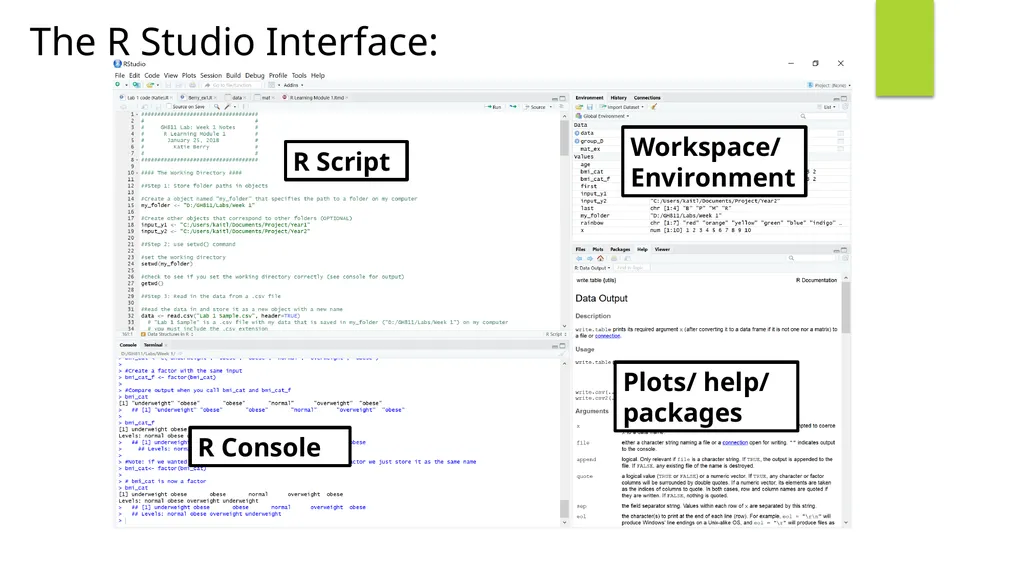
The R Studio Interface: R Script R Console Workspace/ Environment Plots/ help/ packages

R Script Top left corner
Type your code here
Typing in the script allows you to save the script, reopen it, and edit it next time
To open a new script:
File  New File  R Script
Click the first icon that looks like a blank page with a green plus

R Console Bottom left corner
This is where R actually processes and executes code
Output appears here
You can type code here BUT
R runs each line as you type it
Can’t edit command after you hit enter

PLEASE ALWAYS WRITE YOUR CODE IN THE SCRIPT FOR THIS CLASS (not in the console)!

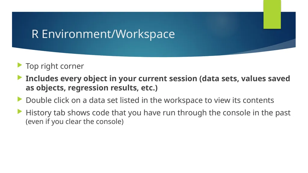
R Environment/Workspace Top right corner
Includes every object in your current session (data sets, values saved as objects, regression results, etc.)
Double click on a data set listed in the workspace to view its contents
History tab shows code that you have run through the console in the past (even if you clear the console)

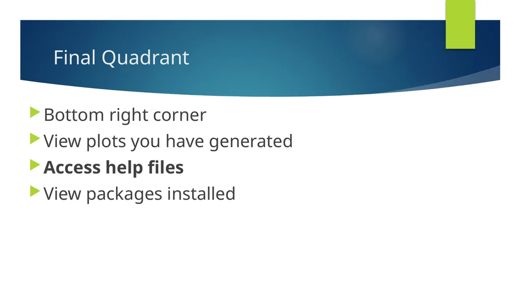
Final Quadrant Bottom right corner
View plots you have generated
Access help files
View packages installed

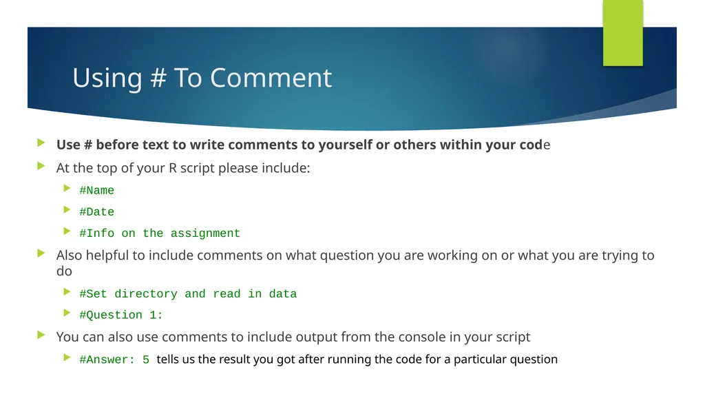
Using # To Comment Use # before text to write comments to yourself or others within your code
At the top of your R script please include:
#Name
#Date
#Info on the assignment
Also helpful to include comments on what question you are working on or what you are trying to do
#Set directory and read in data
#Question 1:
You can also use comments to include output from the console in your script
#Answer: 5 tells us the result you got after running the code for a particular question

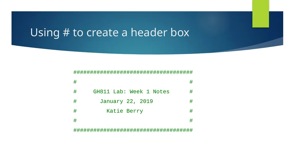
Using # to create a header box ####################################
# #
# GH811 Lab: Week 1 Notes #
# January 22, 2019 #
# Katie Berry #
# #
####################################

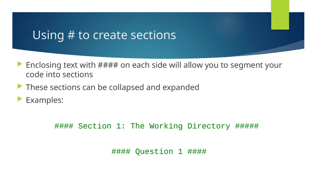
Using # to create sections Enclosing text with #### on each side will allow you to segment your code into sections
These sections can be collapsed and expanded
Examples:

#### Section 1: The Working Directory #####

#### Question 1 ####

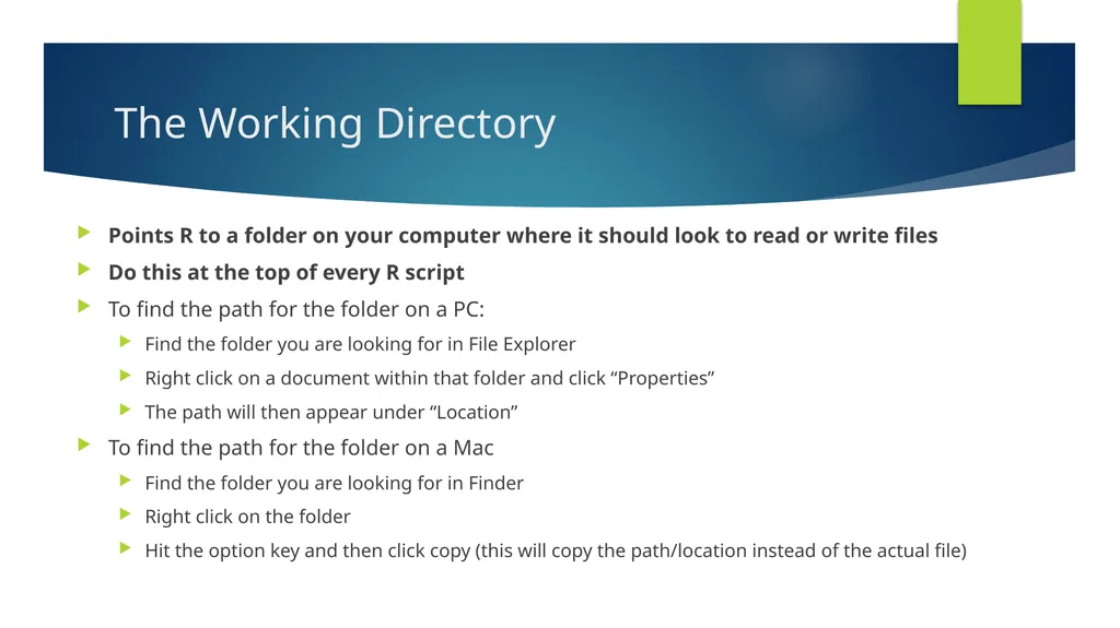
The Working Directory Points R to a folder on your computer where it should look to read or write files
Do this at the top of every R script
To find the path for the folder on a PC:
Find the folder you are looking for in File Explorer
Right click on a document within that folder and click “Properties”
The path will then appear under “Location”
To find the path for the folder on a Mac
Find the folder you are looking for in Finder
Right click on the folder
Hit the option key and then click copy (this will copy the path/location instead of the actual file)

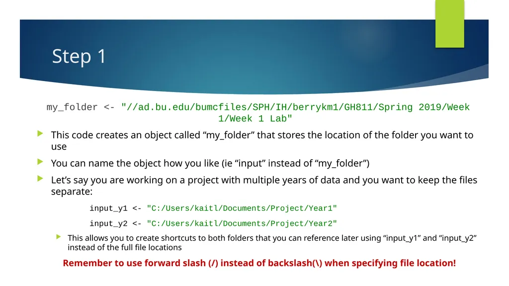
Step 1 my_folder <- "//ad.bu.edu/bumcfiles/SPH/IH/berrykm1/GH811/Spring 2019/Week 1/Week 1 Lab"
This code creates an object called “my_folder” that stores the location of the folder you want to use
You can name the object how you like (ie “input” instead of “my_folder”)
Let’s say you are working on a project with multiple years of data and you want to keep the files separate:
input_y1 <- "C:/Users/kaitl/Documents/Project/Year1"
input_y2 <- "C:/Users/kaitl/Documents/Project/Year2"
This allows you to create shortcuts to both folders that you can reference later using “input_y1” and “input_y2” instead of the full file locations
Remember to use forward slash (/) instead of backslash(\) when specifying file location!

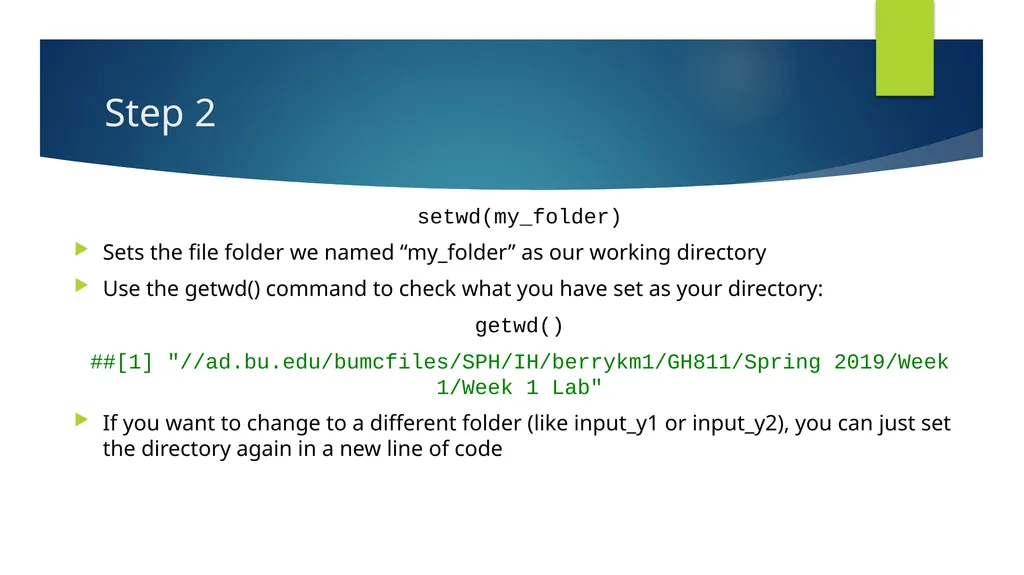
Step 2 setwd(my_folder)
Sets the file folder we named “my_folder” as our working directory
Use the getwd() command to check what you have set as your directory:
getwd()
##[1] "//ad.bu.edu/bumcfiles/SPH/IH/berrykm1/GH811/Spring 2019/Week 1/Week 1 Lab"
If you want to change to a different folder (like input_y1 or input_y2), you can just set the directory again in a new line of code

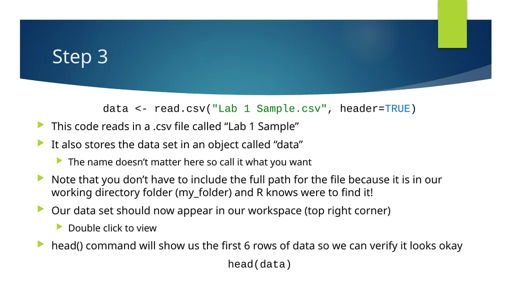
Step 3 data <- read.csv("Lab 1 Sample.csv", header=TRUE)
This code reads in a .csv file called “Lab 1 Sample”
It also stores the data set in an object called “data”
The name doesn’t matter here so call it what you want
Note that you don’t have to include the full path for the file because it is in our working directory folder (my_folder) and R knows were to find it!
Our data set should now appear in our workspace (top right corner)
Double click to view
head() command will show us the first 6 rows of data so we can verify it looks okay
head(data)

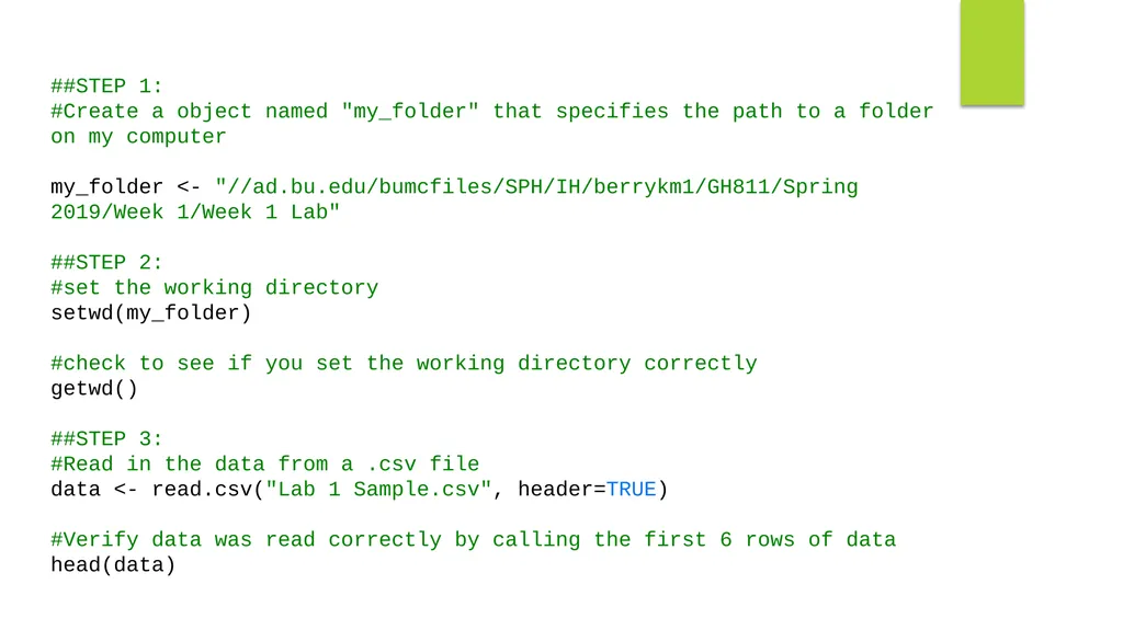
##STEP 1:
#Create a object named "my_folder" that specifies the path to a folder on my computer

my_folder <- "//ad.bu.edu/bumcfiles/SPH/IH/berrykm1/GH811/Spring 2019/Week 1/Week 1 Lab"

##STEP 2:
#set the working directory
setwd(my_folder)

#check to see if you set the working directory correctly
getwd()

##STEP 3:
#Read in the data from a .csv file
data <- read.csv("Lab 1 Sample.csv", header=TRUE)

#Verify data was read correctly by calling the first 6 rows of data
head(data)

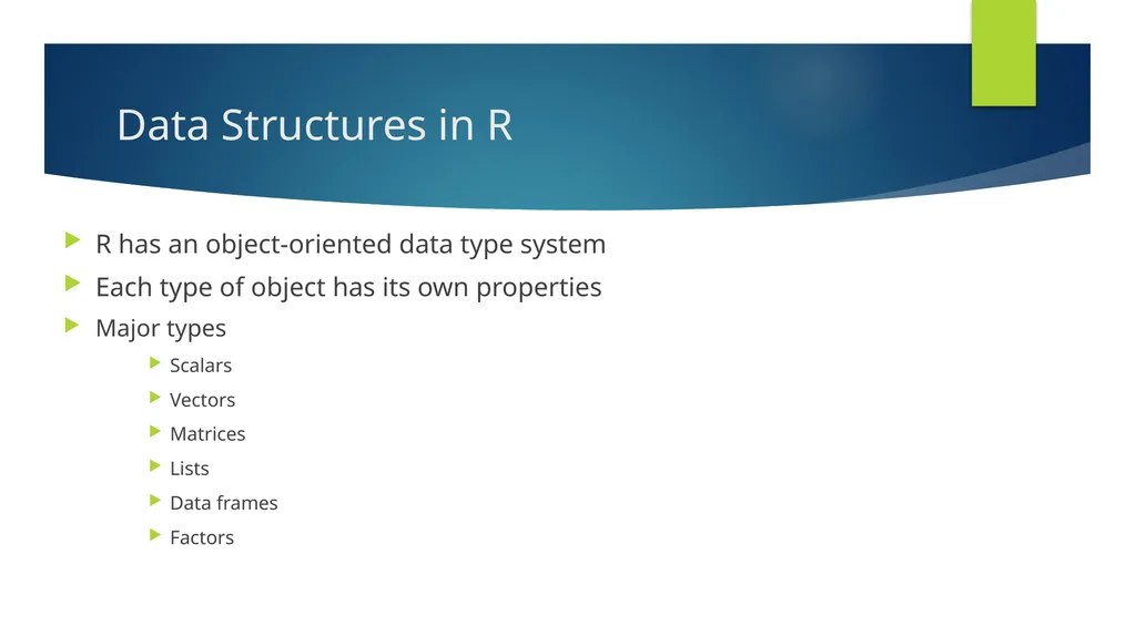
Data Structures in R R has an object-oriented data type system
Each type of object has its own properties
Major types
Scalars
Vectors
Matrices
Lists
Data frames
Factors

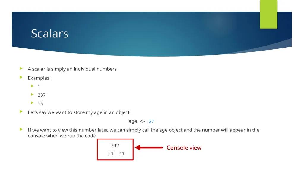
Scalars A scalar is simply an individual numbers
Examples:
1
387
15
Let’s say we want to store my age in an object:
age <- 27
If we want to view this number later, we can simply call the age object and the number will appear in the console when we run the code
age
[1] 27 Console view

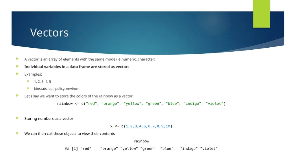
Vectors A vector is an array of elements with the same mode (ie numeric, character)
Individual variables in a data frame are stored as vectors
Examples:
1, 2, 3, 4, 5
biostats, epi, policy, environ
Let’s say we want to store the colors of the rainbow as a vector
rainbow <- c("red", "orange", "yellow", "green", "blue", "indigo", "violet")

Storing numbers as a vector
x <- c(1,2,3,4,5,6,7,8,9,10)
We can then call these objects to view their contents
rainbow
## [1] "red" "orange" "yellow" "green" "blue" "indigo" "violet"

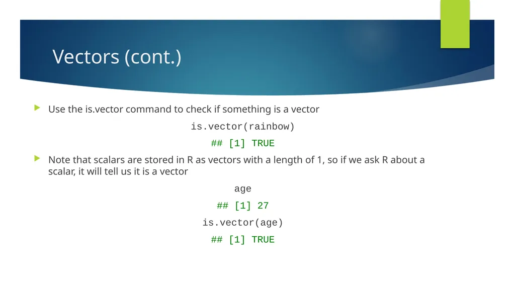
Vectors (cont.) Use the is.vector command to check if something is a vector
is.vector(rainbow)
## [1] TRUE
Note that scalars are stored in R as vectors with a length of 1, so if we ask R about a scalar, it will tell us it is a vector
age
## [1] 27
is.vector(age)
## [1] TRUE

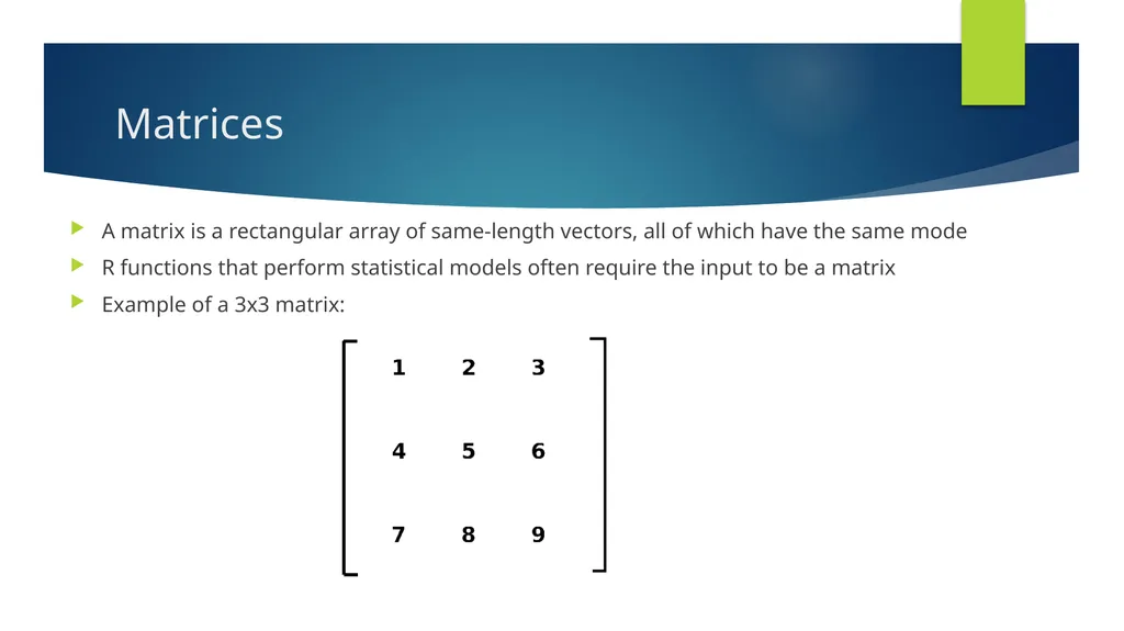
Matrices A matrix is a rectangular array of same-length vectors, all of which have the same mode
R functions that perform statistical models often require the input to be a matrix
Example of a 3x3 matrix:

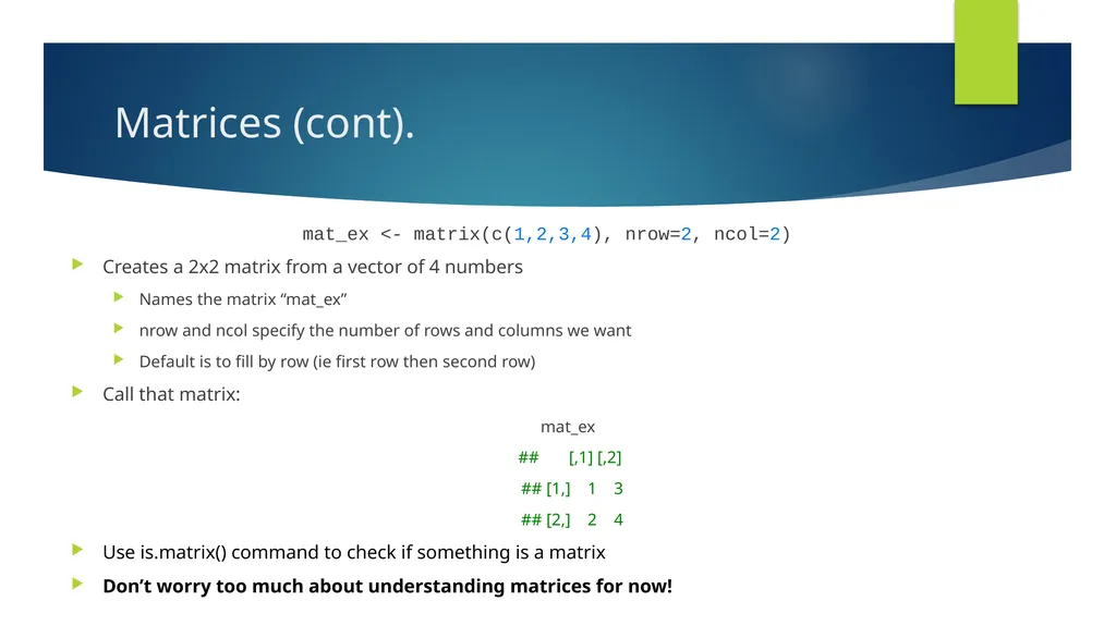
Matrices (cont). mat_ex <- matrix(c(1,2,3,4), nrow=2, ncol=2)
Creates a 2x2 matrix from a vector of 4 numbers
Names the matrix “mat_ex”
nrow and ncol specify the number of rows and columns we want
Default is to fill by row (ie first row then second row)
Call that matrix:
mat_ex
## [,1] [,2]
## [1,] 1 3
## [2,] 2 4
Use is.matrix() command to check if something is a matrix
Don’t worry too much about understanding matrices for now!

Lists A list is a collection of other objects, none of which has to be of the same mode or structure
A list could contain both a character vector and a numeric matrix as separate elements
Many R functions that perform statistical models return the same output as a list containing various components
Don’t worry too much about lists for now!

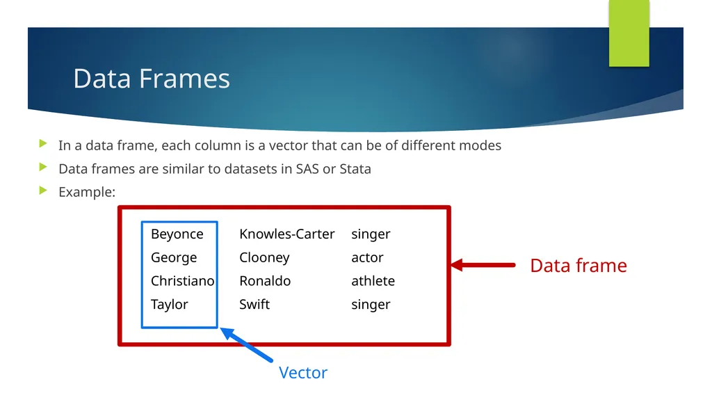
Data Frames In a data frame, each column is a vector that can be of different modes
Data frames are similar to datasets in SAS or Stata
Example: Data frame Vector

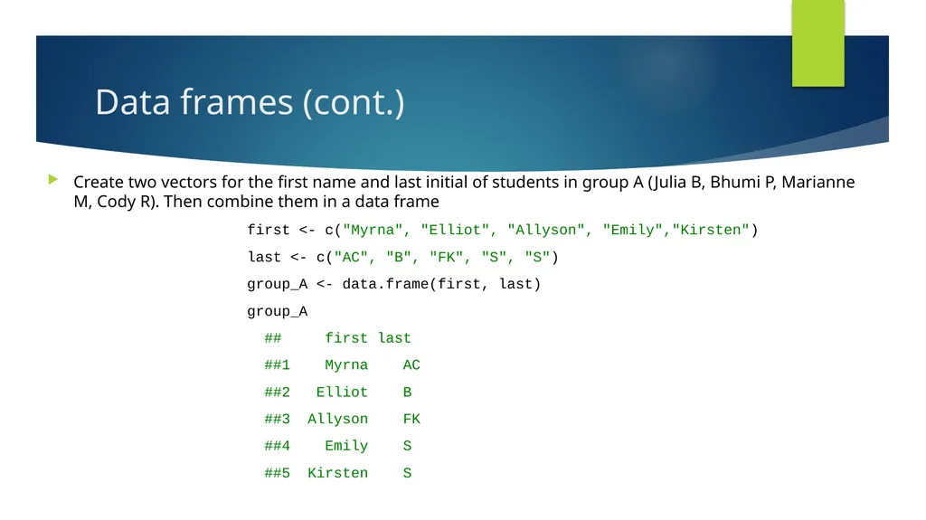
Data frames (cont.) Create two vectors for the first name and last initial of students in group A (Julia B, Bhumi P, Marianne M, Cody R). Then combine them in a data frame
first <- c("Myrna", "Elliot", "Allyson", "Emily","Kirsten")
last <- c("AC", "B", "FK", "S", "S")
group_A <- data.frame(first, last)
group_A
## first last
##1 Myrna AC
##2 Elliot B
##3 Allyson FK
##4 Emily S
##5 Kirsten S

Factors Factors are similar to vectors
BUT factors include a list of its unique values, called levels
Levels are sorted alphabetically for character values
Levels are sorted in ascending order for numeric values
This additional information allows R to perform categorical analyses
Example:
1, 2, 3, 3, 4, 5, 5, 6 is a vector called “x”
1, 2, 3, 4, 5, 6 are its levels if we classify it as a factor called “xf”
Use the factor() command to save a vector as a factor
xf <- factor(x)

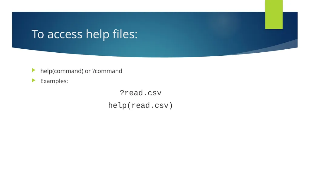
To access help files: help(command) or ?command
Examples:
?read.csv
help(read.csv)

Thanks!berrykm1@bu.edu for questions

R Learning Module 1 GH 811 Lab: Week 1 January

Related Topics

Share

Embed code

Download this presentation From Below

Presentation Transcript