Resource Adequacy Coincident Adjustment Factor Methodology Miguel Cerrutti Demand Analysis Office Energy Assessments Division R.14-10-010 Workshop California Public Utility Commission San Francisco, February 18, 2016 The problem Initiatives
"Resource Adequacy Coincident Adjustment Factor" is the property of its rightful owner. Permission is granted to
download and print the materials on this website for personal, non-commercial use only, and to display it
on your personal computer provided you do not modify the materials and that you retain all copyright
notices contained in the materials. By downloading content from our website, you accept the terms of this
agreement.
Demand Analysis Office
Energy Assessments Division
R.14-10-010 Workshop
California Public Utility Commission
San Francisco, February 18, 2016<br>
02
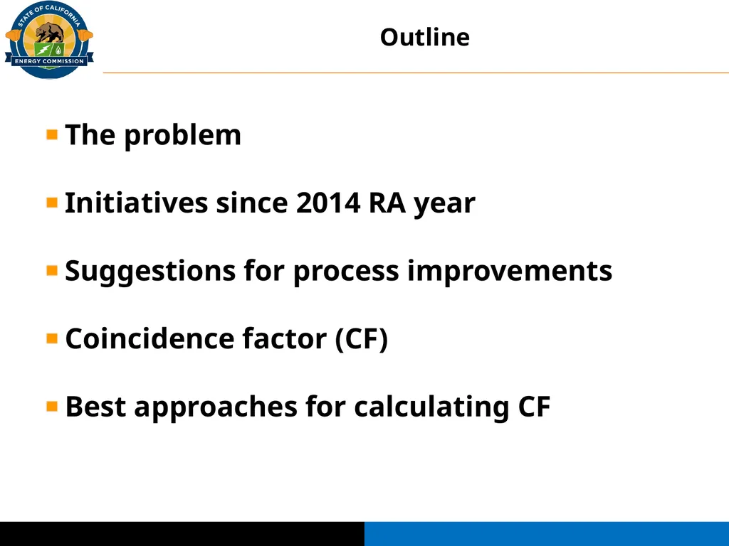
The problem
Initiatives since 2014 RA year
Suggestions for process improvements
Coincidence factor (CF)
Best approaches for calculating CF Outline<br>
03
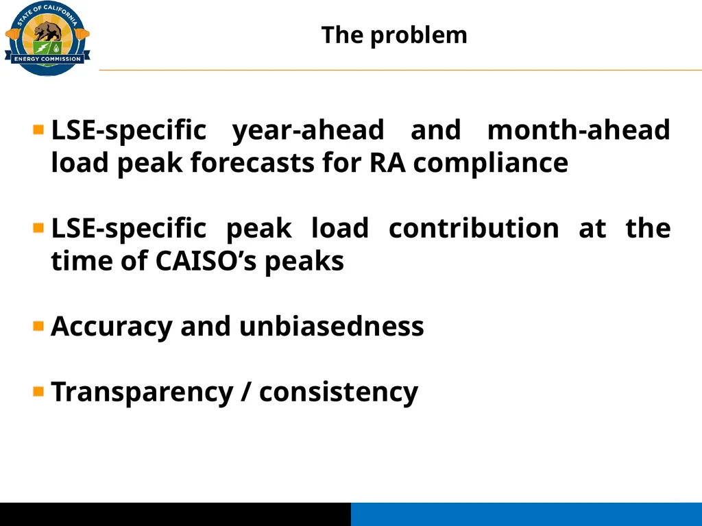
LSE-specific year-ahead and month-ahead load peak forecasts for RA compliance
LSE-specific peak load contribution at the time of CAISO’s peaks
Accuracy and unbiasedness
Transparency / consistency The problem<br>
04
Embedding DR impacts in submitted data
Posting CAISO’s five top monthly coincident peak load dates and hours
Exploring alternative methods
be relatively stable over time
easy to calculate / monitor / apply
Validation - adjustment
load migration
variations in weather and load composition
forecasting an art as much as a science Initiatives since 2014 RA Year<br>
05
Potentially use OASIS data instead of EMS data
OASIS data is not confidential and available sooner
Staff will post five peaks per month for last three years and study use of OASIS data by April 8
Staff will republish manual with criteria on when to use 1, 3, or five peaks per month
Staff will always use last three years of historical data. This translates to either 36 points, 108 points, or 180 points of data
Primary objective is accuracy
Transparency and standardization are secondary objectives Suggestions for process improvements<br>
06
Ratio LSE’s peaks at time of CAISO coincident peaks (CP) to the LSE’s non-coincident peaks (NCP)
how close LSE’s peak dates/hours are to CAISO’s five top monthly peak dates/hours
CAISO’s peaks strongly correlated with RES
LSEs with most RES load - most coincident
cross-subsidization - RES/COM/IND
CAISO’s peaks - capacity to be procured
LSEs capacity obligation / costs Coincidence factor (CF)<br>
07
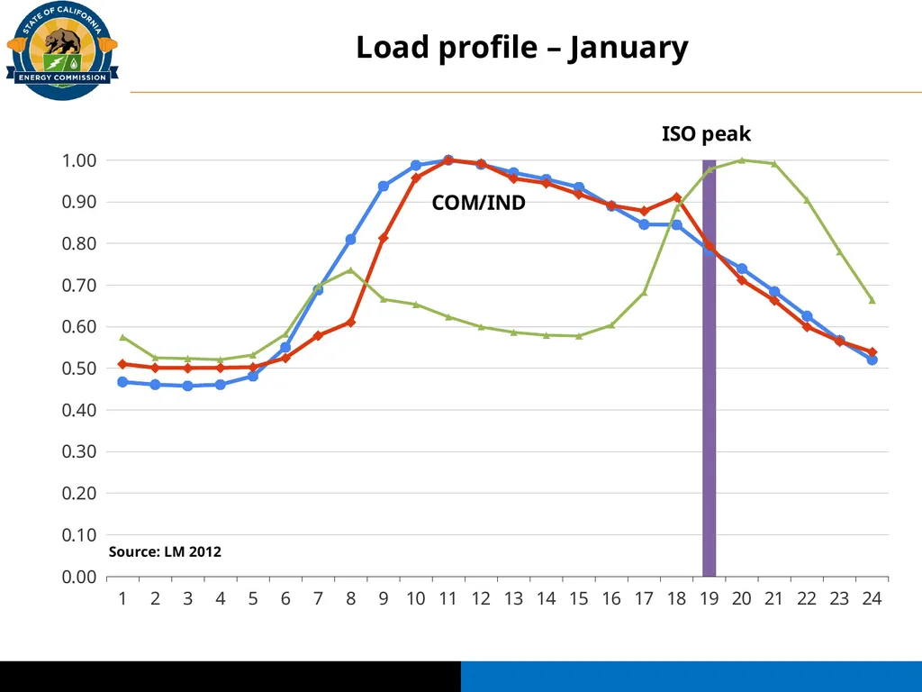
Load profile – January Source: LM 2012<br>
08
LSEs’ load profiles display significant variation across time in load shapes and time of peaks
Hourly loads – time-series
CAISO EMS/OASIS/five top monthly peaks
CPUC jurisdictional/non-jurisdictional LSEs
LSE-specific CF
LSE-composite CF – ESPs/CCAs
load migration and new ESPs/CCAs Coincidence factor (CF)<br>
09
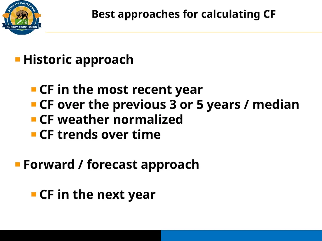
Historic approach
CF in the most recent year
CF over the previous 3 or 5 years / median
CF weather normalized
CF trends over time
Forward / forecast approach
CF in the next year Best approaches for calculating CF<br>
10
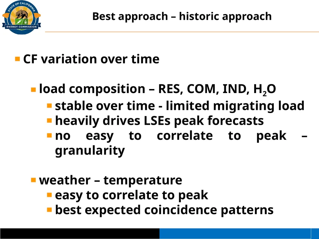
CF variation over time
load composition – RES, COM, IND, H2O
stable over time - limited migrating load
heavily drives LSEs peak forecasts
no easy to correlate to peak – granularity
weather – temperature
easy to correlate to peak
best expected coincidence patterns Best approach – historic approach<br>
11
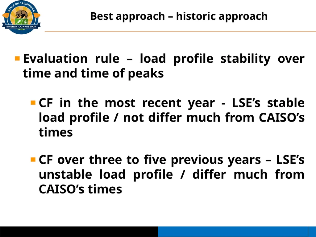
Evaluation rule – load profile stability over time and time of peaks
CF in the most recent year - LSE’s stable load profile / not differ much from CAISO’s times
CF over three to five previous years – LSE’s unstable load profile / differ much from CAISO’s times Best approach – historic approach<br>
12
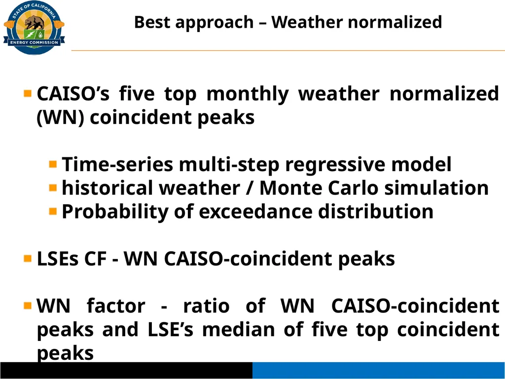
CAISO’s five top monthly weather normalized (WN) coincident peaks
Time-series multi-step regressive model
historical weather / Monte Carlo simulation
Probability of exceedance distribution
LSEs CF - WN CAISO-coincident peaks
WN factor - ratio of WN CAISO-coincident peaks and LSE’s median of five top coincident peaks Best approach – Weather normalized<br>
13
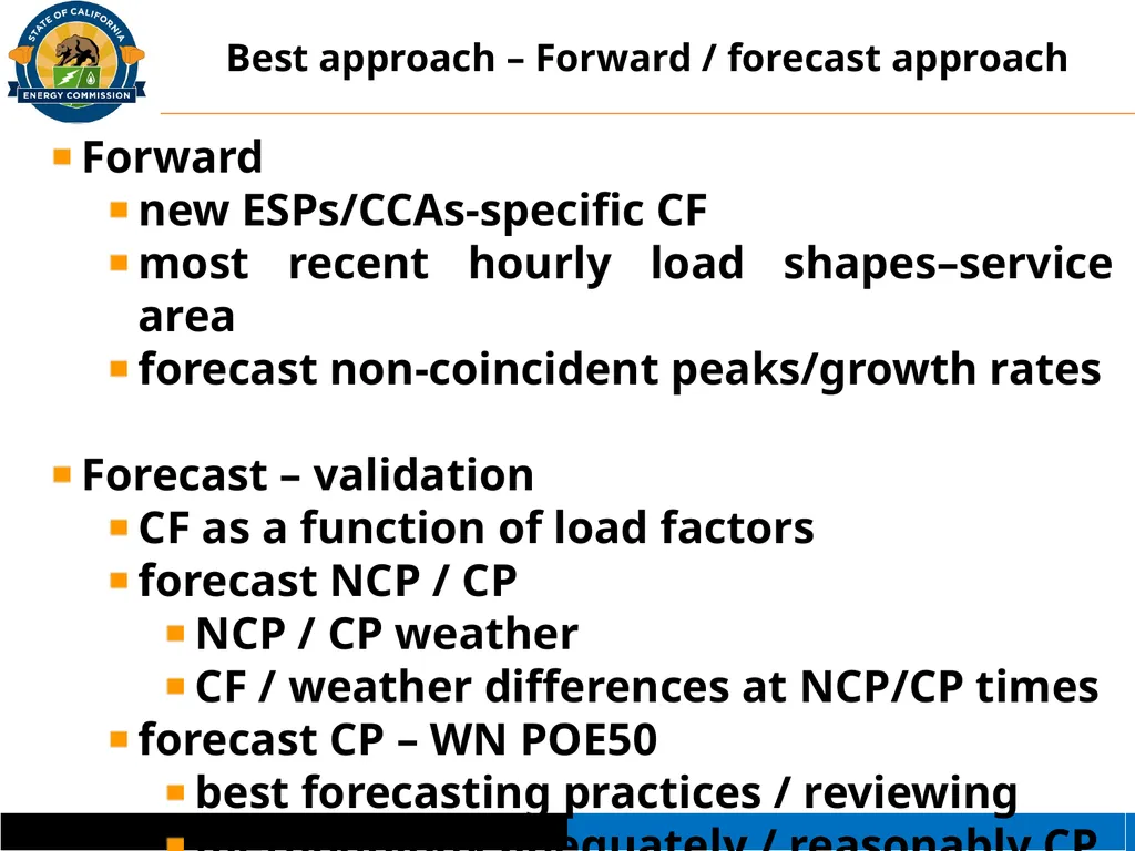
Forward
new ESPs/CCAs-specific CF
most recent hourly load shapes–service area
forecast non-coincident peaks/growth rates
Forecast – validation
CF as a function of load factors
forecast NCP / CP
NCP / CP weather
CF / weather differences at NCP/CP times
forecast CP – WN POE50
best forecasting practices / reviewing
methodology adequately / reasonably CP Best approach – Forward / forecast approach<br>