Risk Neutral Densities: A Review Stephen

slide1. Risk Neutral Densities: A ReviewStephen Figlewski* * Professor of Finance
Stern School of Business
New York University

email: sfiglews@stern.nyu.edu<br>
slide2. I. Overview
II. Options, Probabilities, and Risk Preferences: The P and the Q-densities
III. The Evolution of the Data Generating Process and the Risk Neutral Density
IV. Overview of Estimation Methodology
V. Implied Volatility: The Volatility Risk Premium and the VIX
VI. The Volatility Surface
VII. The "Pricing Kernel Puzzle"
VIII. Two Major Directions for Future Research Outline of Presentation International Risk Management Conference 2018 ©2018 Figlewski<br>
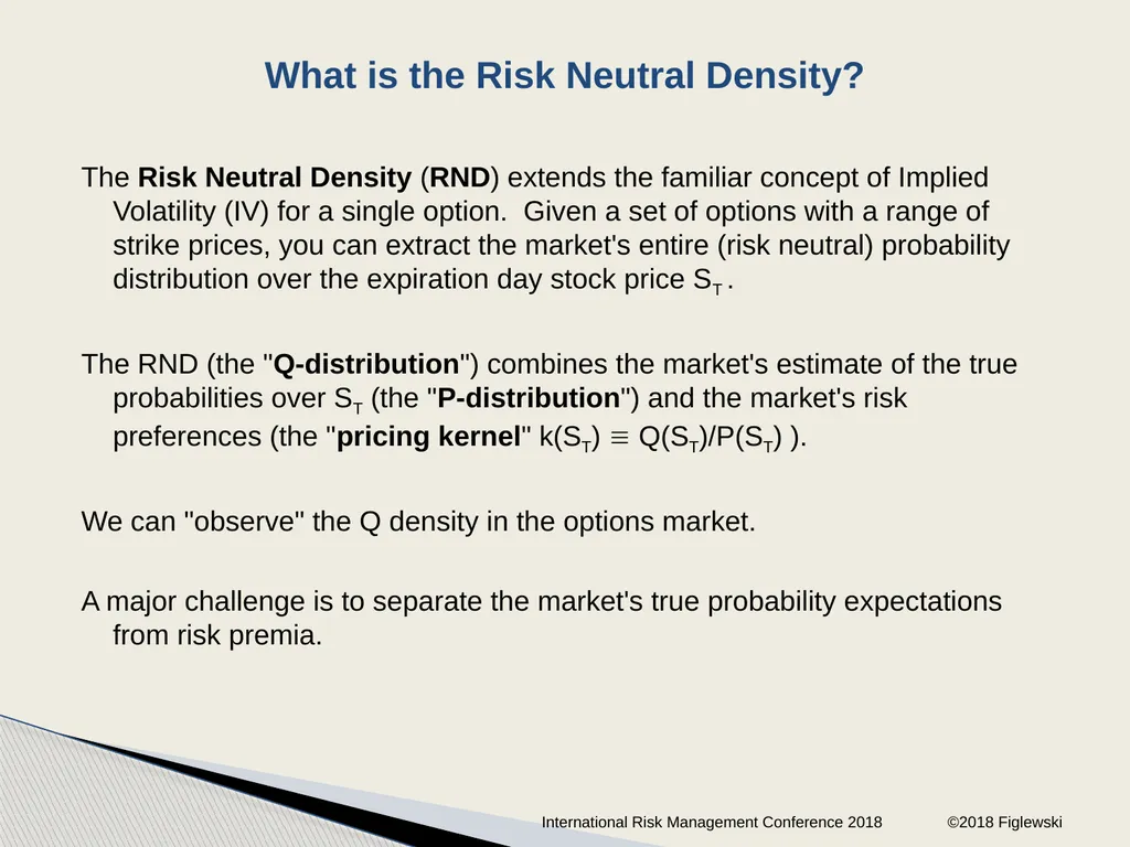
slide3. The Risk Neutral Density (RND) extends the familiar concept of Implied Volatility (IV) for a single option. Given a set of options with a range of strike prices, you can extract the market's entire (risk neutral) probability distribution over the expiration day stock price ST .

The RND (the "Q-distribution") combines the market's estimate of the true probabilities over ST (the "P-distribution") and the market's risk preferences (the "pricing kernel" k(ST)  Q(ST)/P(ST) ).

We can "observe" the Q density in the options market.

A major challenge is to separate the market's true probability expectations from risk premia. What is the Risk Neutral Density? International Risk Management Conference 2018 ©2018 Figlewski<br>
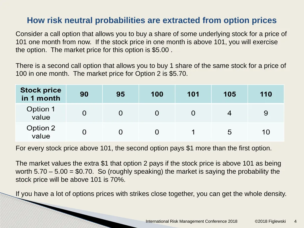
slide4. Consider a call option that allows you to buy a share of some underlying stock for a price of 101 one month from now. If the stock price in one month is above 101, you will exercise the option. The market price for this option is $5.00 .

There is a second call option that allows you to buy 1 share of the same stock for a price of 100 in one month. The market price for Option 2 is $5.70.

For every stock price above 101, the second option pays $1 more than the first option.

The market values the extra $1 that option 2 pays if the stock price is above 101 as being worth 5.70 – 5.00 = $0.70. So (roughly speaking) the market is saying the probability the stock price will be above 101 is 70%.

If you have a lot of options prices with strikes close together, you can get the whole density. How risk neutral probabilities are extracted from option prices 4 International Risk Management Conference 2018 ©2018 Figlewski<br>
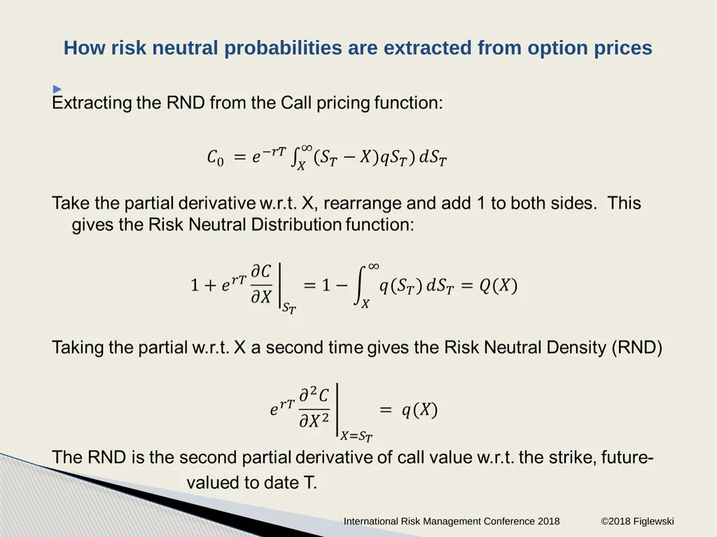
slide5. How risk neutral probabilities are extracted from option prices International Risk Management Conference 2018 ©2018 Figlewski<br>
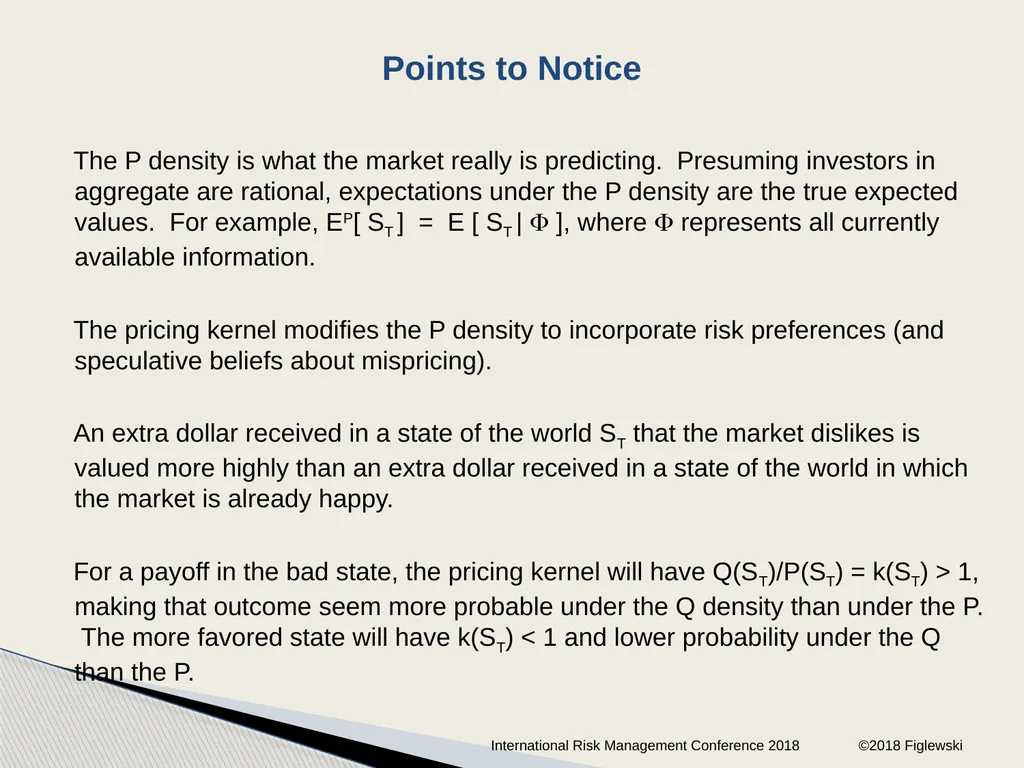
slide6. The P density is what the market really is predicting. Presuming investors in aggregate are rational, expectations under the P density are the true expected values. For example, EP[ ST ] = E [ ST |  ], where  represents all currently available information.

The pricing kernel modifies the P density to incorporate risk preferences (and speculative beliefs about mispricing).

An extra dollar received in a state of the world ST that the market dislikes is valued more highly than an extra dollar received in a state of the world in which the market is already happy.

For a payoff in the bad state, the pricing kernel will have Q(ST)/P(ST) = k(ST) > 1, making that outcome seem more probable under the Q density than under the P. The more favored state will have k(ST) < 1 and lower probability under the Q than the P. Points to Notice International Risk Management Conference 2018 ©2018 Figlewski<br>
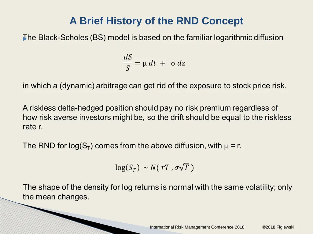
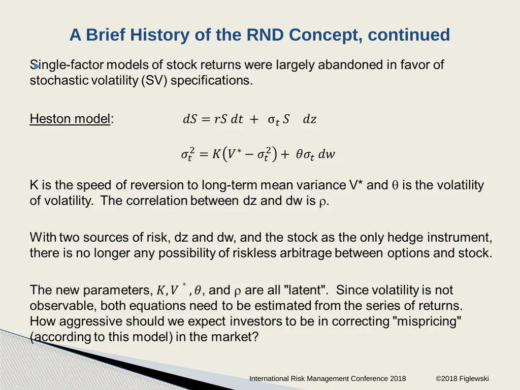
slide7. A Brief History of the RND Concept International Risk Management Conference 2018 ©2018 Figlewski<br>
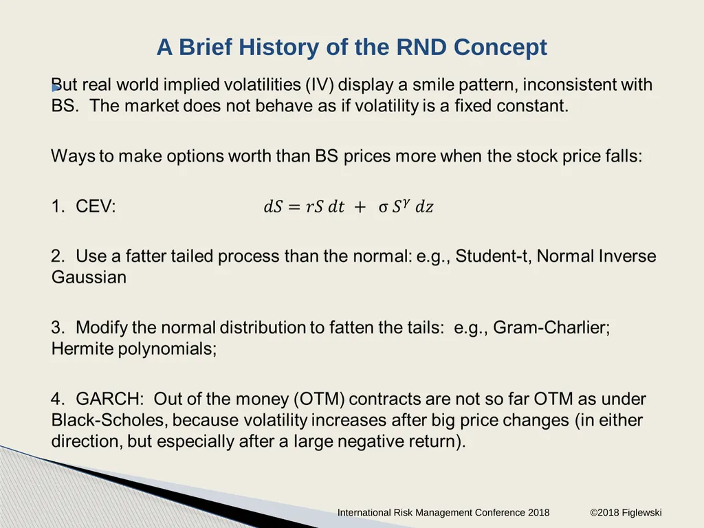
slide8. A Brief History of the RND Concept International Risk Management Conference 2018 ©2018 Figlewski<br>
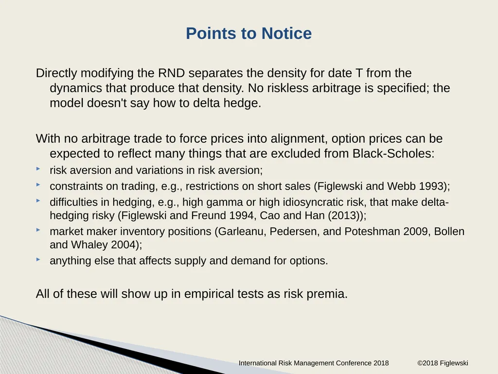
slide9. Directly modifying the RND separates the density for date T from the dynamics that produce that density. No riskless arbitrage is specified; the model doesn't say how to delta hedge.

With no arbitrage trade to force prices into alignment, option prices can be expected to reflect many things that are excluded from Black-Scholes:
risk aversion and variations in risk aversion;
constraints on trading, e.g., restrictions on short sales (Figlewski and Webb 1993);
difficulties in hedging, e.g., high gamma or high idiosyncratic risk, that make delta-hedging risky (Figlewski and Freund 1994, Cao and Han (2013));
market maker inventory positions (Garleanu, Pedersen, and Poteshman 2009, Bollen and Whaley 2004);
anything else that affects supply and demand for options.

All of these will show up in empirical tests as risk premia. Points to Notice International Risk Management Conference 2018 ©2018 Figlewski<br>
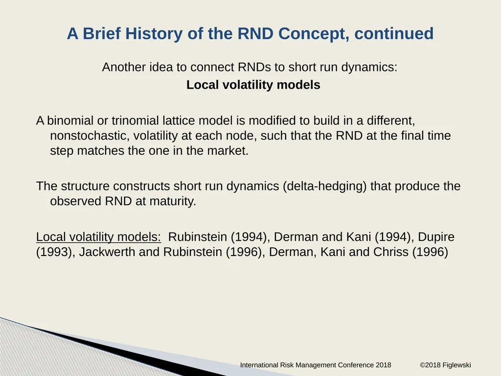
slide10. Another idea to connect RNDs to short run dynamics:
Local volatility models

A binomial or trinomial lattice model is modified to build in a different, nonstochastic, volatility at each node, such that the RND at the final time step matches the one in the market.

The structure constructs short run dynamics (delta-hedging) that produce the observed RND at maturity.

Local volatility models: Rubinstein (1994), Derman and Kani (1994), Dupire (1993), Jackwerth and Rubinstein (1996), Derman, Kani and Chriss (1996) A Brief History of the RND Concept, continued International Risk Management Conference 2018 ©2018 Figlewski<br>
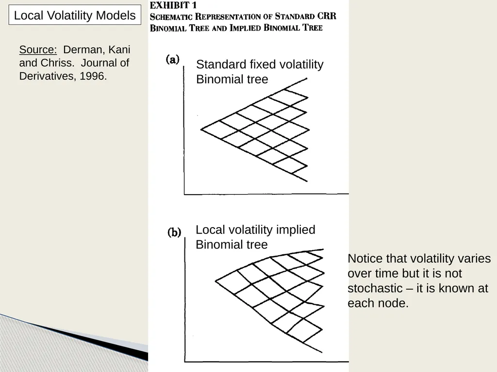
slide11. title Local Volatility Models Standard fixed volatility
Binomial tree Local volatility implied
Binomial tree Source: Derman, Kani
and Chriss. Journal of
Derivatives, 1996. Notice that volatility varies
over time but it is not
stochastic – it is known at
each node.<br>
slide12. Local volatility models

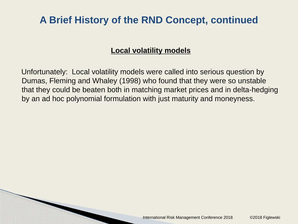
Unfortunately: Local volatility models were called into serious question by Dumas, Fleming and Whaley (1998) who found that they were so unstable that they could be beaten both in matching market prices and in delta-hedging by an ad hoc polynomial formulation with just maturity and moneyness. A Brief History of the RND Concept, continued International Risk Management Conference 2018 ©2018 Figlewski<br>
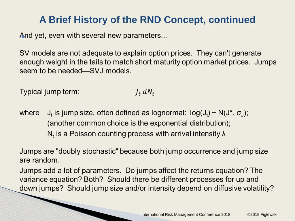
slide13. A Brief History of the RND Concept, continued International Risk Management Conference 2018 ©2018 Figlewski<br>
slide14. A Brief History of the RND Concept, continued International Risk Management Conference 2018 ©2018 Figlewski<br>
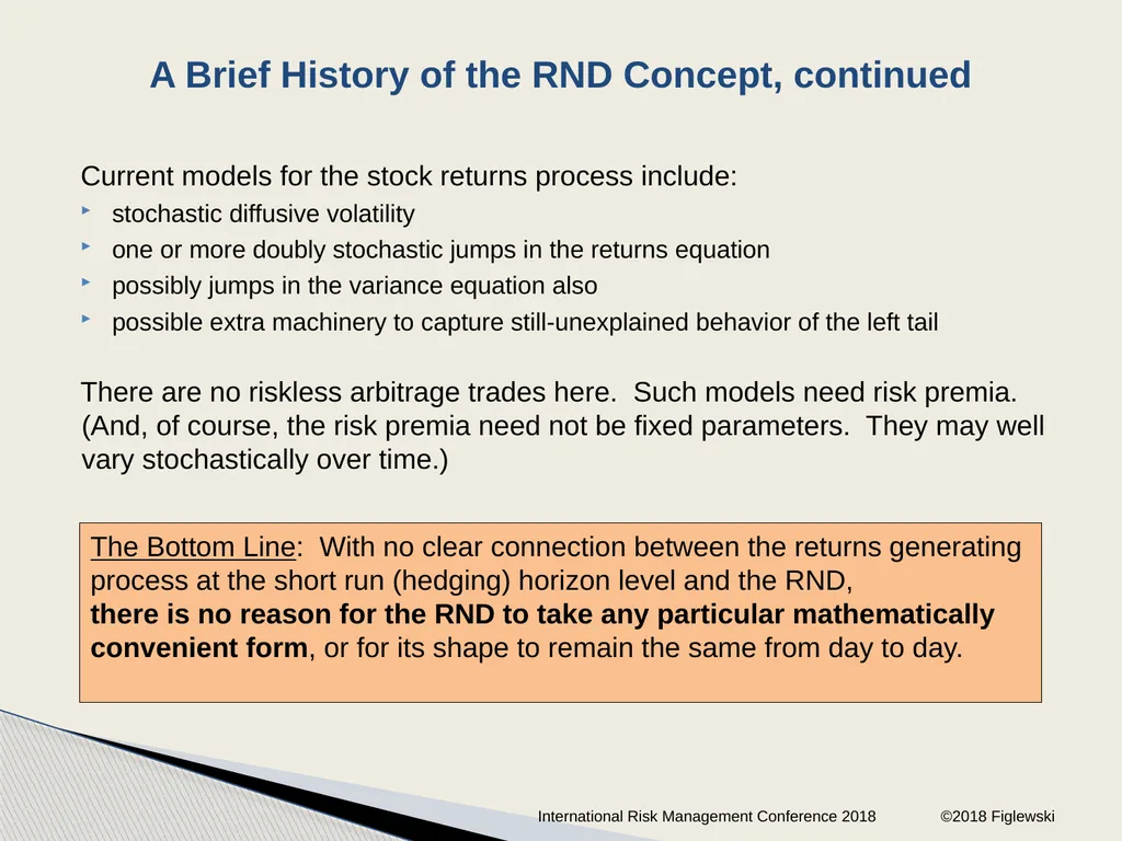
slide15. Current models for the stock returns process include:
stochastic diffusive volatility
one or more doubly stochastic jumps in the returns equation
possibly jumps in the variance equation also
possible extra machinery to capture still-unexplained behavior of the left tail

There are no riskless arbitrage trades here. Such models need risk premia. (And, of course, the risk premia need not be fixed parameters. They may well vary stochastically over time.) A Brief History of the RND Concept, continued International Risk Management Conference 2018 ©2018 Figlewski The Bottom Line: With no clear connection between the returns generating
process at the short run (hedging) horizon level and the RND,
there is no reason for the RND to take any particular mathematically
convenient form, or for its shape to remain the same from day to day.<br>
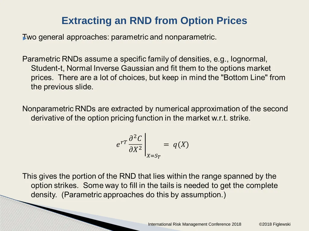
slide16. Extracting an RND from Option Prices International Risk Management Conference 2018 ©2018 Figlewski<br>
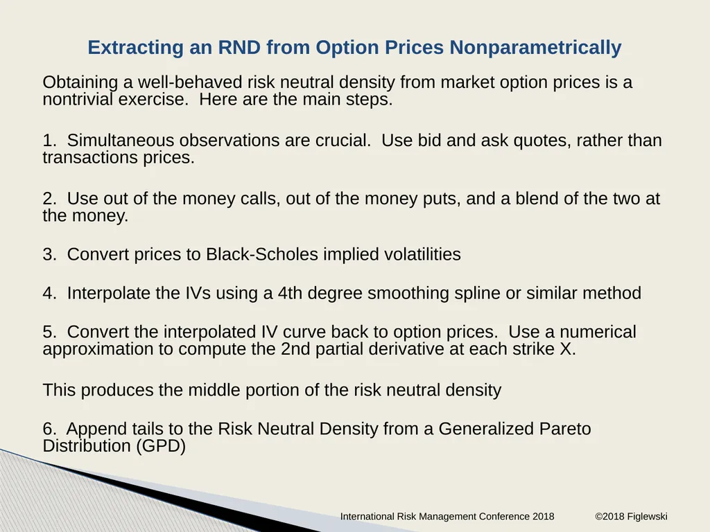
slide17. Obtaining a well-behaved risk neutral density from market option prices is a nontrivial exercise. Here are the main steps.

1. Simultaneous observations are crucial. Use bid and ask quotes, rather than transactions prices.

2. Use out of the money calls, out of the money puts, and a blend of the two at the money.

3. Convert prices to Black-Scholes implied volatilities

4. Interpolate the IVs using a 4th degree smoothing spline or similar method

5. Convert the interpolated IV curve back to option prices. Use a numerical approximation to compute the 2nd partial derivative at each strike X.

This produces the middle portion of the risk neutral density

6. Append tails to the Risk Neutral Density from a Generalized Pareto Distribution (GPD) Extracting an RND from Option Prices Nonparametrically International Risk Management Conference 2018 ©2018 Figlewski<br>
slide18. stuff International Risk Management Conference 2018 ©2018 Figlewski<br>
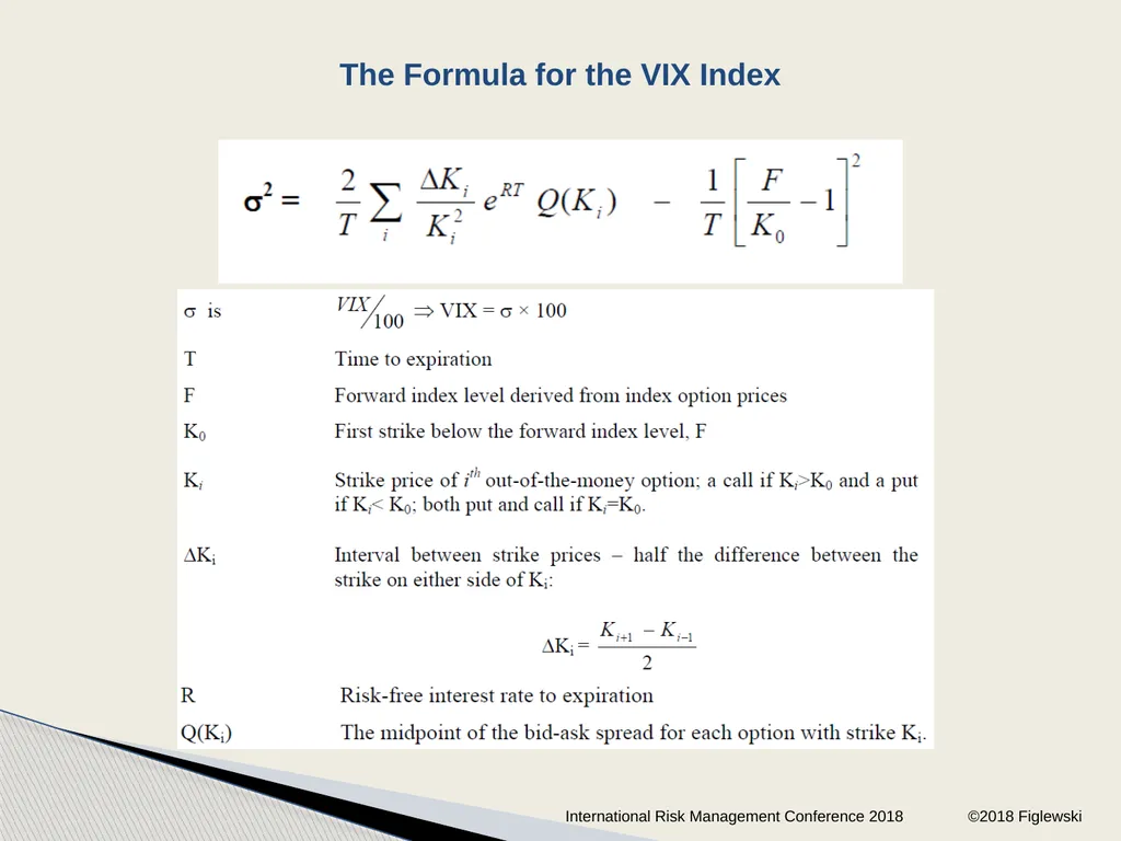
slide19. Bakshi, Kapadia, and Madan (Review of Financial Studies, 2003) derived formulas for the moments of an approximated RND in terms of the underlying option prices.

Given the first 4 moments, a parametric RND can be easily fitted to the observed option prices.

The moments may be of interest by themselves, in particular the volatility. The formula became the basis for the new VIX index. Extracting an RND from Option Prices International Risk Management Conference 2018 ©2018 Figlewski<br>
slide20. The Formula for the VIX Index International Risk Management Conference 2018 ©2018 Figlewski<br>
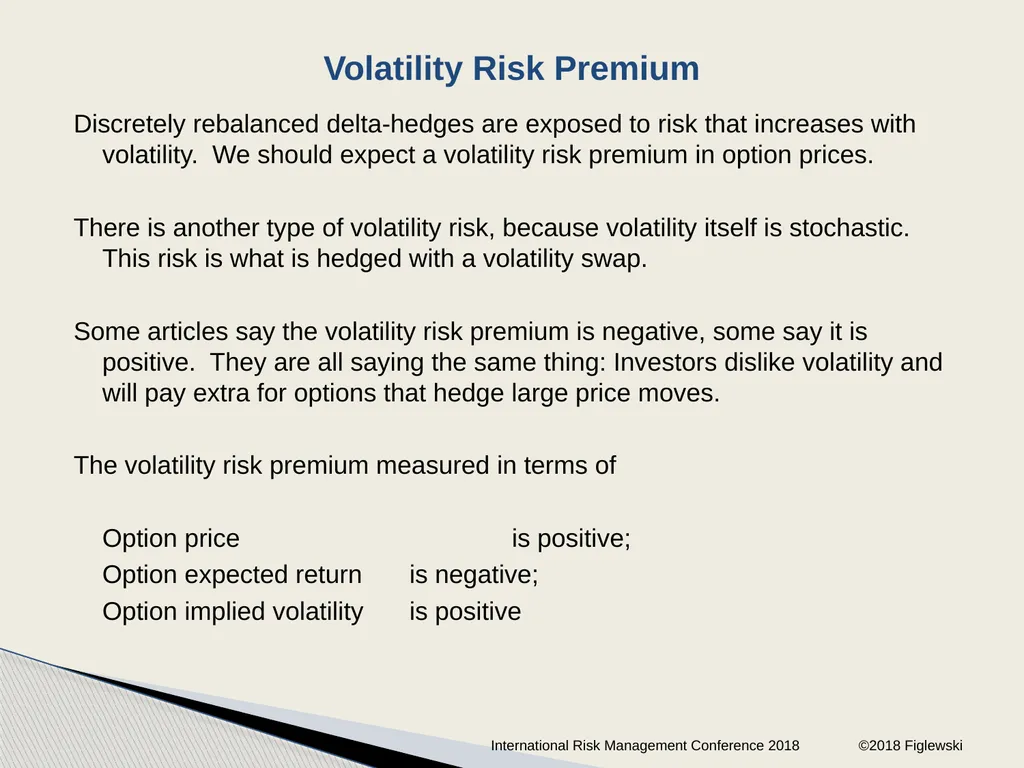
slide21. Discretely rebalanced delta-hedges are exposed to risk that increases with volatility. We should expect a volatility risk premium in option prices.

There is another type of volatility risk, because volatility itself is stochastic. This risk is what is hedged with a volatility swap.

Some articles say the volatility risk premium is negative, some say it is positive. They are all saying the same thing: Investors dislike volatility and will pay extra for options that hedge large price moves.

The volatility risk premium measured in terms of

Option price is positive;
Option expected return is negative;
Option implied volatility is positive Volatility Risk Premium International Risk Management Conference 2018 ©2018 Figlewski<br>
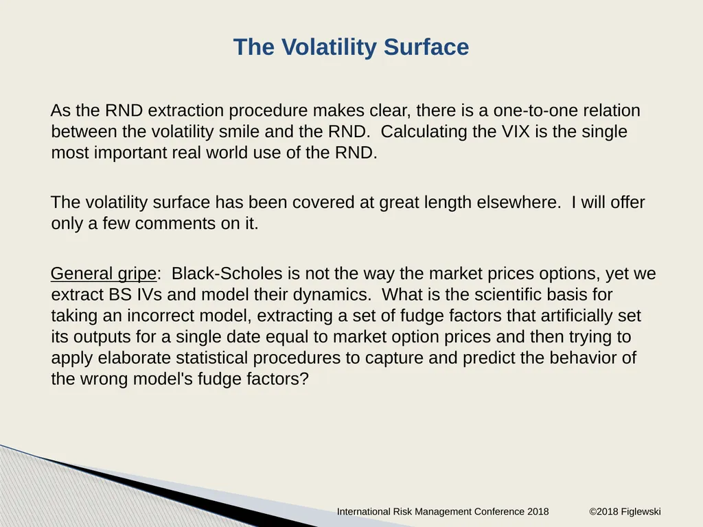
slide22. As the RND extraction procedure makes clear, there is a one-to-one relation between the volatility smile and the RND. Calculating the VIX is the single most important real world use of the RND.

The volatility surface has been covered at great length elsewhere. I will offer only a few comments on it.

General gripe: Black-Scholes is not the way the market prices options, yet we extract BS IVs and model their dynamics. What is the scientific basis for taking an incorrect model, extracting a set of fudge factors that artificially set its outputs for a single date equal to market option prices and then trying to apply elaborate statistical procedures to capture and predict the behavior of the wrong model's fudge factors? The Volatility Surface International Risk Management Conference 2018 ©2018 Figlewski<br>
slide23. Numerous models of the dynamics of the volatility surface have been proposed.

Articles:
Dumas, Fleming and Whaley (1998)
Cont, da Fonseca, and Durrleman (2001)
Andersen, Fusari and Todorov (2013)
Carr and Wu (2016)
Israelov and Kelly (2017)

Books:
Gatheral (2006)
Derman and Miller (2016) The Volatility Surface International Risk Management Conference 2018 ©2018 Figlewski<br>
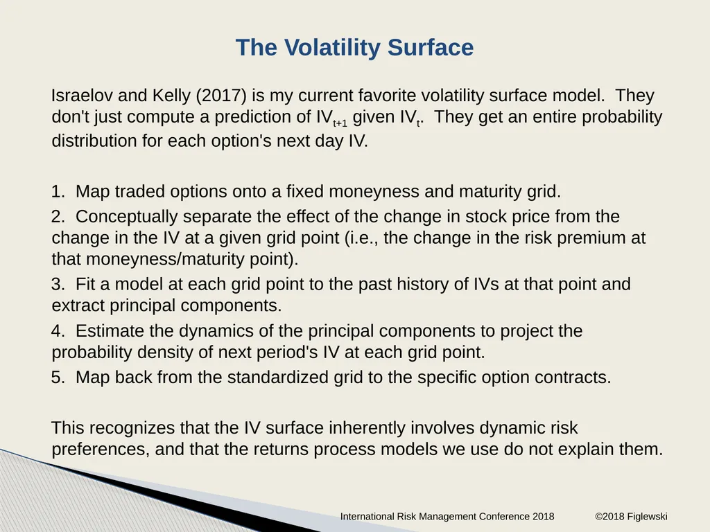
slide24. Israelov and Kelly (2017) is my current favorite volatility surface model. They don't just compute a prediction of IVt+1 given IVt. They get an entire probability distribution for each option's next day IV.

1. Map traded options onto a fixed moneyness and maturity grid.
2. Conceptually separate the effect of the change in stock price from the change in the IV at a given grid point (i.e., the change in the risk premium at that moneyness/maturity point).
3. Fit a model at each grid point to the past history of IVs at that point and extract principal components.
4. Estimate the dynamics of the principal components to project the probability density of next period's IV at each grid point.
5. Map back from the standardized grid to the specific option contracts.

This recognizes that the IV surface inherently involves dynamic risk preferences, and that the returns process models we use do not explain them. The Volatility Surface International Risk Management Conference 2018 ©2018 Figlewski<br>
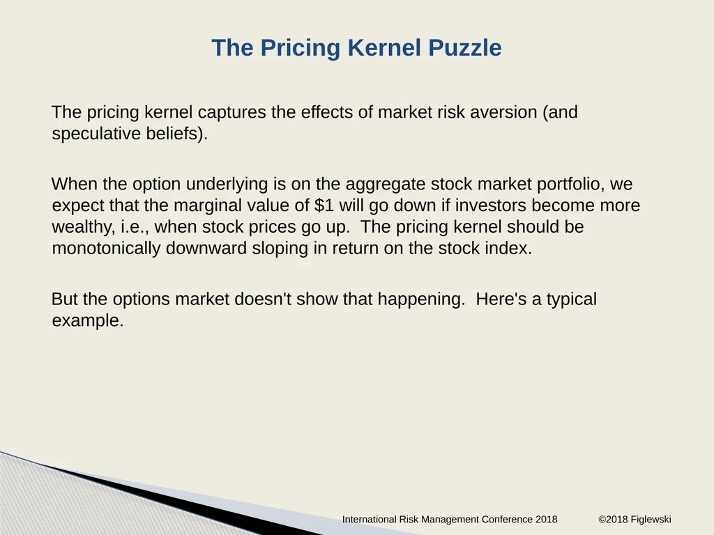
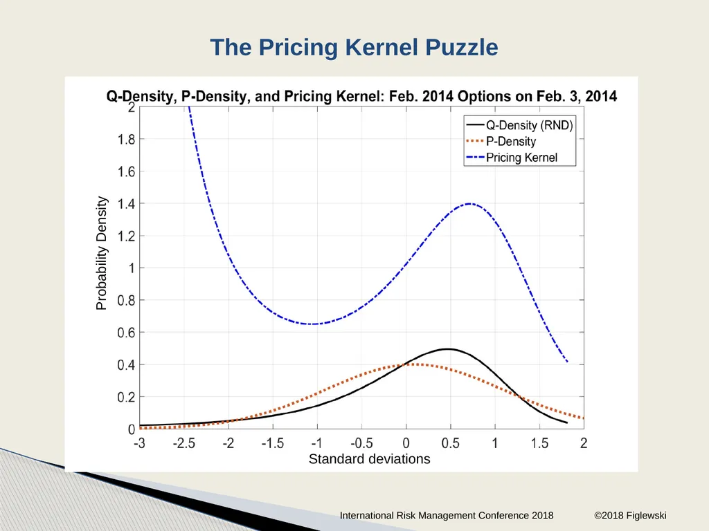
slide25. The pricing kernel captures the effects of market risk aversion (and speculative beliefs).

When the option underlying is on the aggregate stock market portfolio, we expect that the marginal value of $1 will go down if investors become more wealthy, i.e., when stock prices go up. The pricing kernel should be monotonically downward sloping in return on the stock index.

But the options market doesn't show that happening. Here's a typical example. The Pricing Kernel Puzzle International Risk Management Conference 2018 ©2018 Figlewski<br>
slide26. The Pricing Kernel Puzzle International Risk Management Conference 2018 ©2018 Figlewski Standard deviations Probability Density<br>
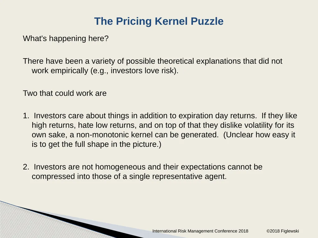
slide27. What's happening here?

There have been a variety of possible theoretical explanations that did not work empirically (e.g., investors love risk).

Two that could work are

1. Investors care about things in addition to expiration day returns. If they like high returns, hate low returns, and on top of that they dislike volatility for its own sake, a non-monotonic kernel can be generated. (Unclear how easy it is to get the full shape in the picture.)

2. Investors are not homogeneous and their expectations cannot be compressed into those of a single representative agent. The Pricing Kernel Puzzle International Risk Management Conference 2018 ©2018 Figlewski<br>
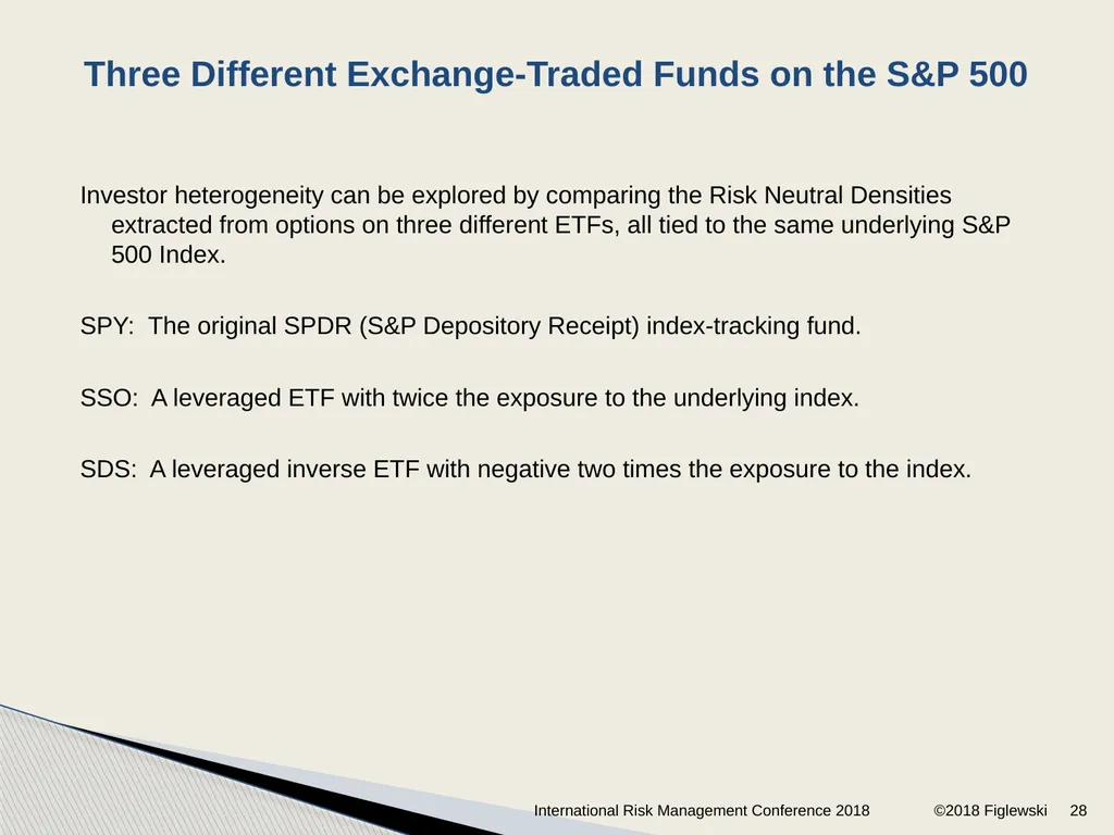
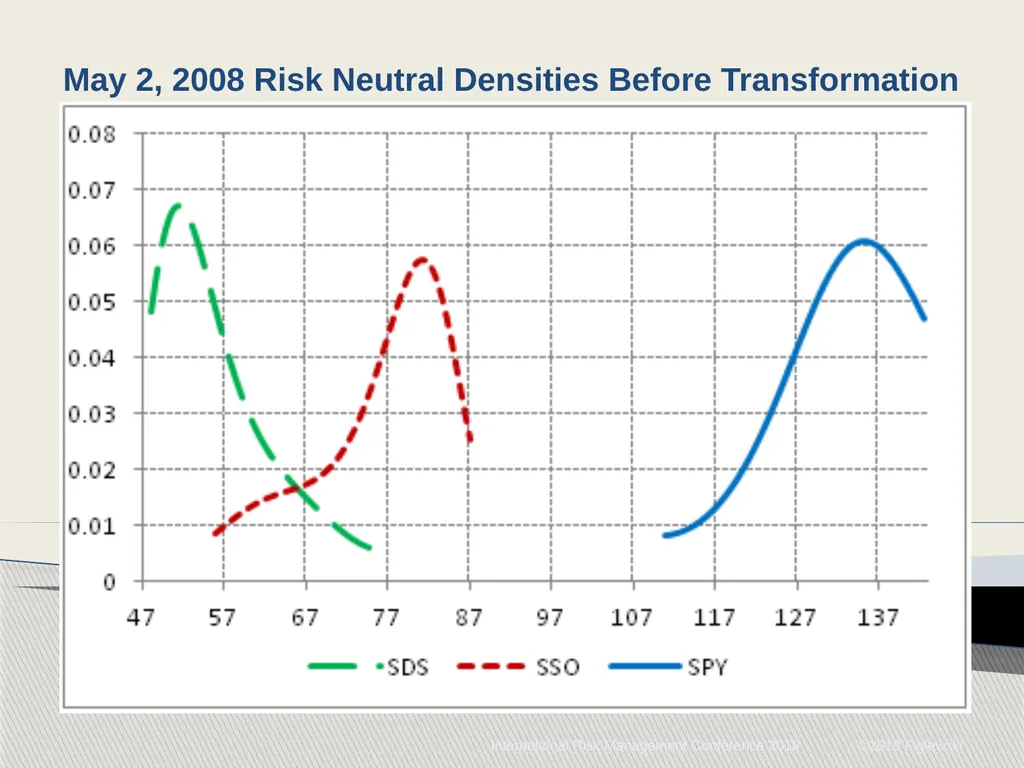
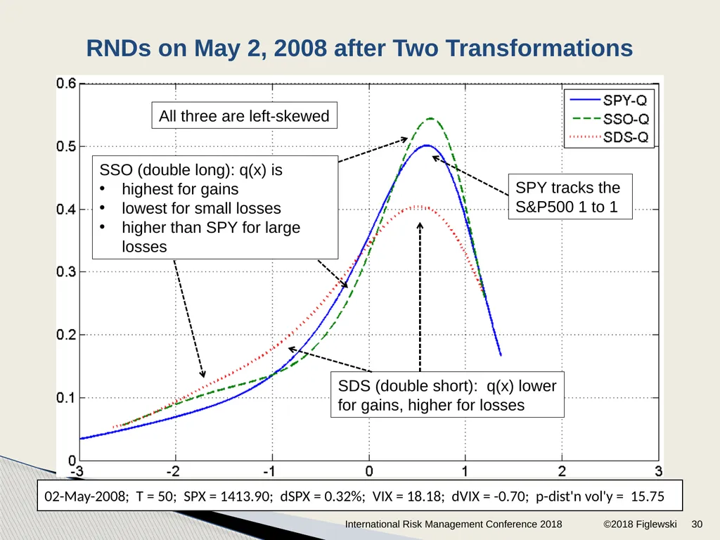
slide28. Investor heterogeneity can be explored by comparing the Risk Neutral Densities extracted from options on three different ETFs, all tied to the same underlying S&P 500 Index.

SPY: The original SPDR (S&P Depository Receipt) index-tracking fund.

SSO: A leveraged ETF with twice the exposure to the underlying index.

SDS: A leveraged inverse ETF with negative two times the exposure to the index. Three Different Exchange-Traded Funds on the S&P 500 28 International Risk Management Conference 2018 ©2018 Figlewski<br>
slide29. May 2, 2008 Risk Neutral Densities Before Transformation International Risk Management Conference 2018 ©2018 Figlewski<br>
slide30. RNDs on May 2, 2008 after Two Transformations 02-May-2008; T = 50; SPX = 1413.90; dSPX = 0.32%; VIX = 18.18; dVIX = -0.70; p-dist'n vol'y = 15.75 30 All three are left-skewed International Risk Management Conference 2018 ©2018 Figlewski<br>
slide31. Two major areas in which theories about Risk Neutral Densities are plainly inadequate, and more research is needed:

Understanding the risk neutralization process: We have gone about as far as we can with models that focus only on the dynamics of the returns process. Option prices, and RNDs, reflect market risk aversion/tolerance, that we have so far made little effort to model in any systematic way.

Allowing for heterogeneous investors: The "representative investor" simplification cannot work for zero-sum contracts like options, futures, and other derivatives. These markets exist in order to transfer risk from one counterparty to another. If investors are identical, they won't trade. They will agree on the option price, but it will be the level where no one wants to take a long or short position. In short, none of our models really capture what any investor in options is actually doing.

There is plenty of room for further research on Risk Neutral Densities! More Research is Needed! International Risk Management Conference 2018 ©2018 Figlewski<br>
slide32. And when you do great new papers on RNDs, send them to the Journal of Derivatives!

THANKS! International Risk Management Conference 2018 ©2018 Figlewski<br>