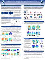
Figure 1: show a causal chain for how Joule heating occurs - PowerPoint Presentation

Slide1

Figure 1: show a causal chain for how Joule heating occurs in the earth’s ionosphere

Figure 5: Is of the same format as figure four but the left panels show the North-South current densities and the right panels show the East-West current densities.

Using

the coupled OpenGGCM-CTIM model we

study the

effect of particle precipitation on the joule heating of the earth’s ionosphere-thermosphere system. We have run two simulations with all parameter identical with one difference between the two; we have set the incoming particle precipitation from the magnetosphere to zero. Granted this is a unphysical view, as it can usually be assumed that the loss cone is filled and that precipitation occurs all the time with a fair amount of variability, but it rarely if ever ceases completely

.

The

intent for these simulations is to compare the difference for electron density

, conductance

current densities, and Joule heating. This causal chain is shown in figure 1. As we compare

the precipitating and non-precipitating case we can gain insights into how

Joule

heating

is effected,

as

well as many other physical processes that could be compared (such as

ionospheric

convection or tail reconnection for example) that are beyond the scope of this poster.

Introduction

Case Study 7 Nov 2004

We

take as a case study the storm event on the 7th of November 2004. Figure 2 shows the solar wind parameters. There are 2 large shocks that occur at 9:20 UT and 18:20 UT (at ACE) previous to the time we have chosen to output our figures at 18:50 UT after the 2nd shock has hits the magnetosphere. This series of shocks led to a major storm that reached a minimum

Dst

of -374.

Figure 2: shows the solar wind parameters for the 7 November storm taken from ACE data

Case Study 7 Nov 2004

Including Precipitation

Precipitation Removed

Electron Density Ratio at 150 km

the noon

midnight meridian. The precipitation effects can be seen in the plots and effects regions down well into the E-region. Again the greatest change is in the

nightside

ionosphere.

Figure 3: Shows a plot of the northern hemisphere the top three panels are in Solar Magnetosphere coordinates. These plots show an altitude slice at 150 km in the ionosphere. The bottom panels show the noon midnight meridian and plot the altitudinal variation from 100-500 km. The left panels show the simulation where particle precipitation is calculated normally. The center panels show the simulation where precipitation is turned off. The right most panels show a ratio of the two fields. The gap in the center corresponds to the geographic north pole.

Electron densities

As

particles cascade into the ionosphere most of their energy is transmitted to neutral particles in the form of collisions, these result in more ions and electrons. Figure 3 shows an example of the precipitation event on 7 November 2015. Particle precipitation around the auroral oval (10-20 degrees colatitude from magnetic poles) has increased dramatically. The greatest increase can be seen on the night side as the photoionization process has stopped and the ratio of the two simulations has the greatest change on the night side.

Figure

3 also has an altitude profile of the electron densities. This is

taken from

Electron Density

Figure 4: Shows the conductivities in the ionosphere. The top left 3 panels show the

pederson

conductivities at 150 km with precipitation, without precipitation, and the ratio. The bottom three left panels show the Pederson conductivities height profile along the noon midnight meridian, again with, without and a ratio. The right panels have the same format but are of the Hall conductivities.

Conductivities

The

conductivity in the earth's ionosphere is changed with the increase in electron densities. This creates a more conducting ionosphere that will in turn change how currents flow in

the

ionosphere. The conductivities have a linear relationship with electron densities and as such in the models they follow closely the increase in densities as shown in figure 4. The altitude dependence is also shown and again the night side has the greatest difference as precipitation is the main ionizing influence.

Conductivity

Current Densities

Figure 5 shows a plot of the current densities for north-south, and east-west components. In the precipitating case the magnitudes of current density are greater by an order of magnitude than that of the non-precipitating case. Also the current density is much more enhanced in the night side as anticipated. The currents rearrange in the polar cap region but they do not necessarily close where the increased conductivity is. Altitude dependent plots are shown, for both north-south east-west plots and the differences can be seen clearly. The current system on the night side permit more current to close.

Current Density

J

The

CTIM model calculates Joule heating from the current densities and the electric fields.

The Joule heating is the process whereby electrical energy is converted to mechanical energy. Figure

6 shows the

Joule

heating as calculated by CTIM, again we have an order of magnitude increase in frictional heating that extends over a greater area of the polar cap.

Joule Heating

Precipitation Effects on Joule Heating and Neutral Densities of the Polar Ionosphere

Authors: Joseph B.

Jensen

1

,

Jimmy

Raeder

1

1.University of New Hampshire, Space Science Center, Durham NH, USA

Figure 6: Is of the same format as figure 3 but shows the Joule heating rate at 150km. The expansion of the Joule heating over the whole auroral oval especially on the night side.

References

-Li

, W., D.

Knipp

, J. Lei, and J. Raeder (2011), The relation between dayside local

Poynting

flux enhancement and cusp reconnection, J.

Geophys

. Res., 116, A08301, doi:10.1029/

2011JA016566.

-Raeder, J. (2003), Global

magnetohydrodynamics

—A tutorial, in Space Plasma Simulation, Lecture Notes in Physics, vol. 615, edited by J.

Büchner

, C. T. Dum, and M.

Scholer

, pp. 212–246, Springer, Berlin, doi

:10.1007/3-540-36530-3_11.sdf

Summary

Electron

precipitation

has a

large impact on the earth's ionosphere resulting in increases in electron densities, conductivities, current densities,

Joule

heating and neutral densities. With these modeling tools we

plan to

investigate in the future

some of the basic physics on how precipitation affects

ionospheric

convection patterns, how precipitation affects

magnetotail

dynamics,

and

magnetospheric

convection.

Summary

Current Densities

The neutral densities have a typical change pattern. As energy is converted from electromagnetic to mechanical the ionosphere is heated up causing the neutral particles to expand. This can most easily be seen in the altitudinal plots in the bottom left, the topmost pressure layer of the atmosphere rose more than 40 km. The differences in the pressure layer themselves are shown on the top plots an there is some 10% variation within the layer themselves. Mostly a decrease in the density in the precipitation case. This is probably due to the rising pressure layer has less particles than the cold dense lower pressure layer. The actual density at any given altitude is going to increase.

Neutral Densities

Figure 7:

Graphs of the Neutral density of the same format as figure 3. Note that this is a graph of the pressure levels in the ionosphere, not the absolute altitude.