Section 1.5: Algorithms for Solving Graph Problems
Description: Section 1.5: Algorithms for Solving Graph Problems Math for Liberal Studies Brute Force is Hard! As we have seen, the brute force method can require us to examine a very large number of circuits In this section we will develop algorithms
Related Topics
Download Presentation
"Section 1.5: Algorithms for Solving Graph Problems" is the property of its rightful owner. Permission is granted to download and print the materials on this website for personal, non-commercial use only, and to display it on your personal computer provided you do not modify the materials and that you retain all copyright notices contained in the materials. By downloading content from our website, you accept the terms of this agreement.
Presentation Transcript
slide1. Section 1.5: Algorithms for Solving Graph Problems Math for Liberal Studies<br>
slide2. Brute Force is Hard! As we have seen, the brute force method can require us to examine a very large number of circuits
In this section we will develop algorithms for finding an answer much more quickly
The downside is that we will no longer be guaranteed to have the best possible answer<br>
slide3. Nearest-Neighbor Algorithm The first algorithm we will consider is called the nearest-neighbor algorithm
It’s based on a common sense idea: at each vertex, choose the closest vertex that you haven’t visited yet<br>
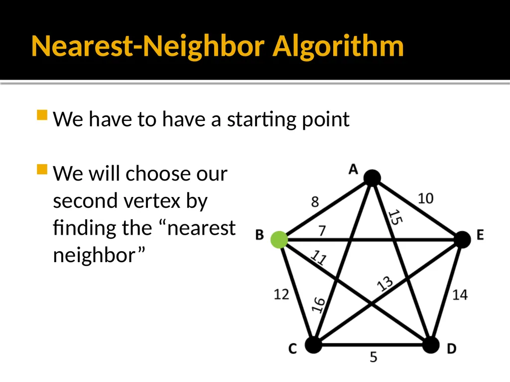
slide4. Nearest-Neighbor Algorithm We have to have a starting point
We will choose oursecond vertex byfinding the “nearestneighbor”<br>
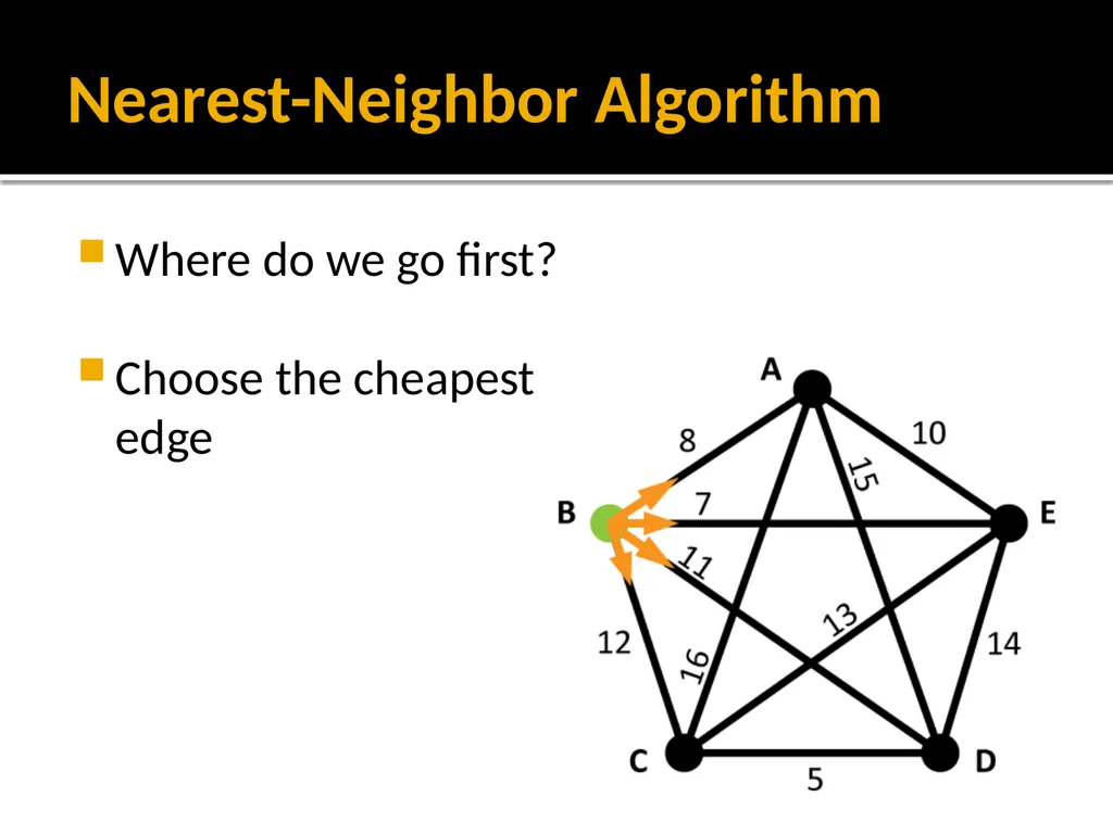
slide5. Nearest-Neighbor Algorithm Where do we go first?
Choose the cheapest edge<br>
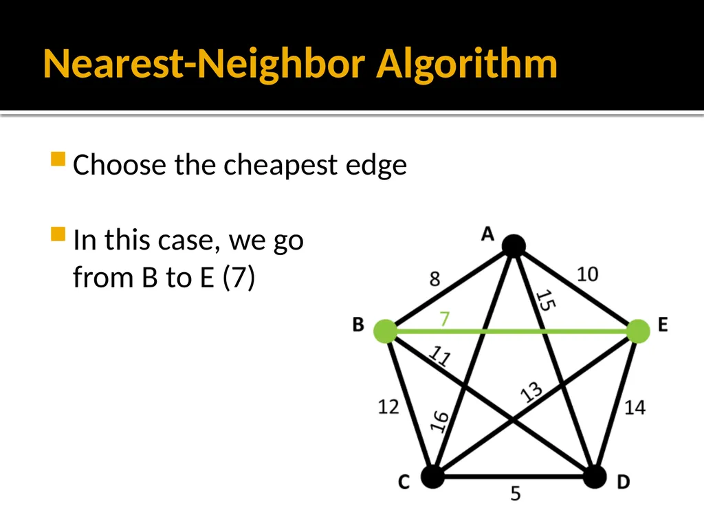
slide6. Nearest-Neighbor Algorithm Choose the cheapest edge
In this case, we gofrom B to E (7)<br>
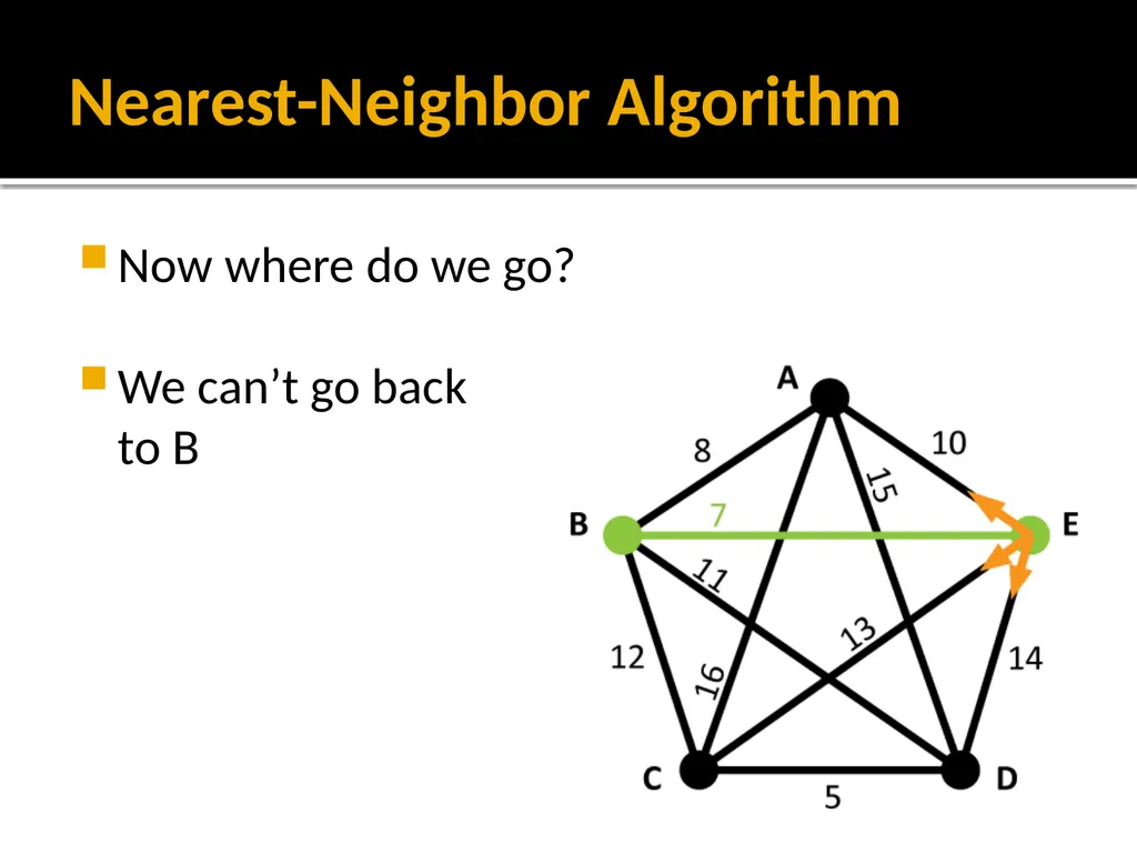
slide7. Nearest-Neighbor Algorithm Now where do we go?
We can’t go backto B<br>
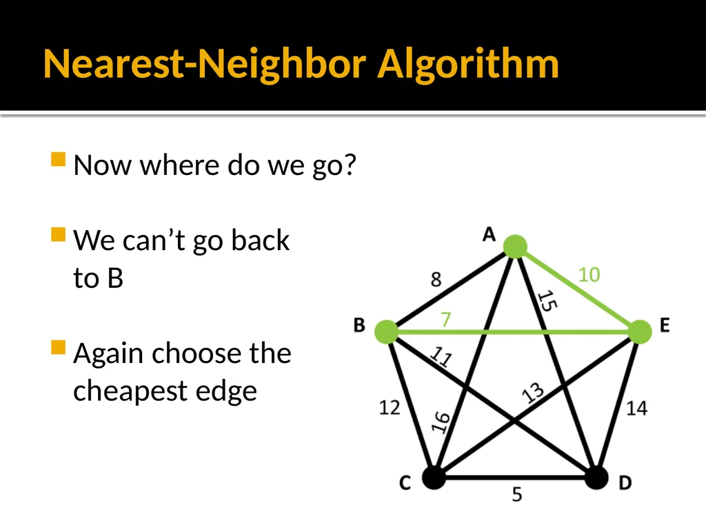
slide8. Nearest-Neighbor Algorithm Now where do we go?
We can’t go backto B
Again choose thecheapest edge<br>
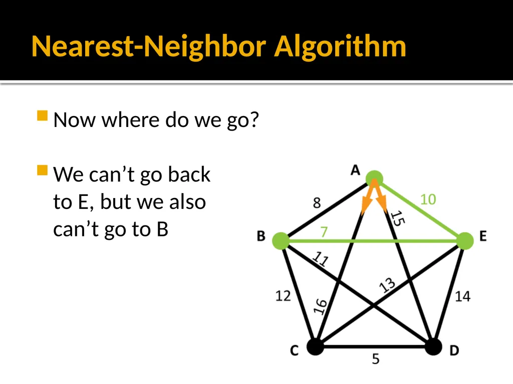
slide9. Nearest-Neighbor Algorithm Now where do we go?
We can’t go backto E, but we alsocan’t go to B<br>
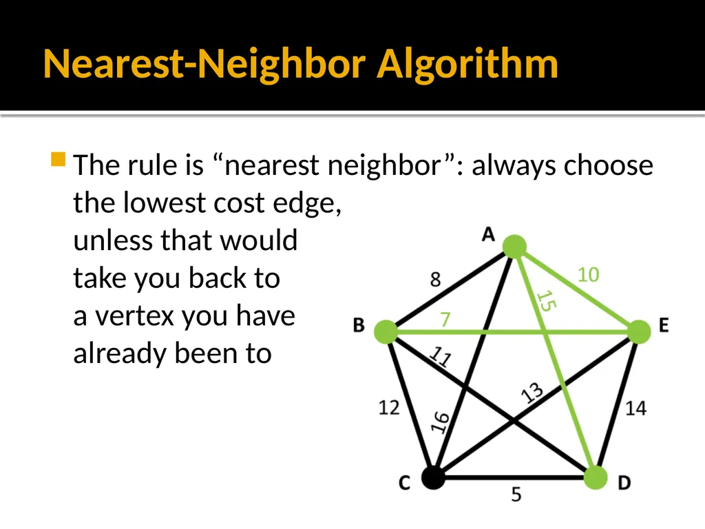
slide10. Nearest-Neighbor Algorithm The rule is “nearest neighbor”: always choose the lowest cost edge, unless that would take you back toa vertex you have already been to<br>
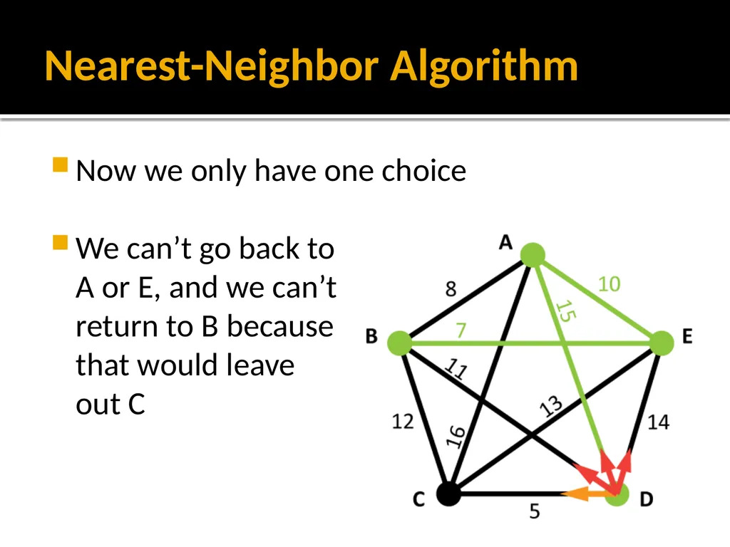
slide11. Nearest-Neighbor Algorithm Now we only have one choice
We can’t go back toA or E, and we can’treturn to B becausethat would leave out C<br>
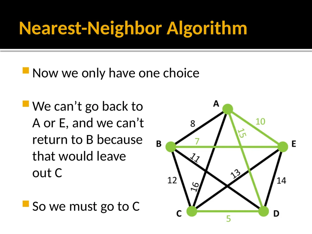
slide12. Nearest-Neighbor Algorithm Now we only have one choice
We can’t go back toA or E, and we can’treturn to B becausethat would leave out C
So we must go to C<br>
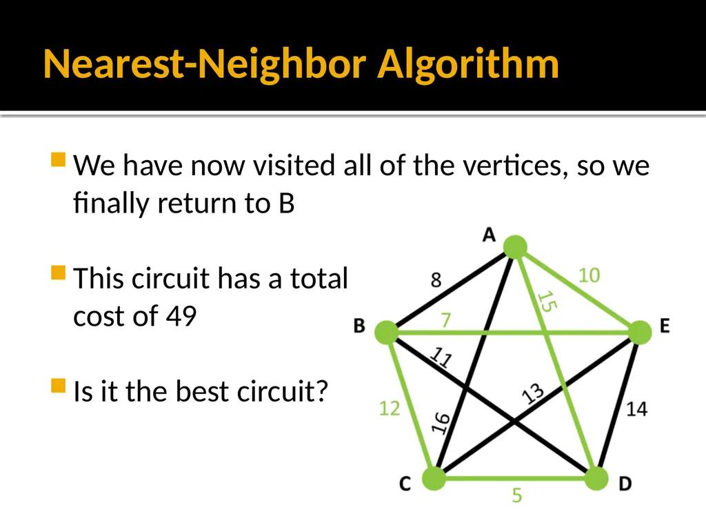
slide13. Nearest-Neighbor Algorithm We have now visited all of the vertices, so we finally return to B
This circuit has a totalcost of 49
Is it the best circuit?<br>
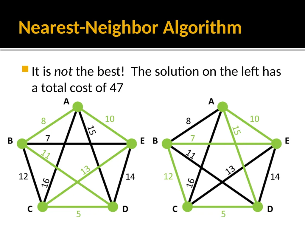
slide14. Nearest-Neighbor Algorithm It is not the best! The solution on the left has a total cost of 47<br>
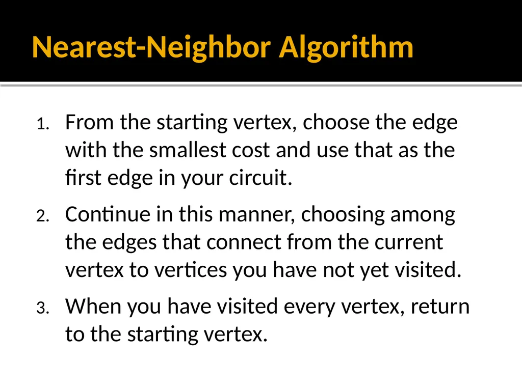
slide15. Nearest-Neighbor Algorithm From the starting vertex, choose the edge with the smallest cost and use that as the first edge in your circuit.
Continue in this manner, choosing among the edges that connect from the current vertex to vertices you have not yet visited.
When you have visited every vertex, return to the starting vertex.<br>
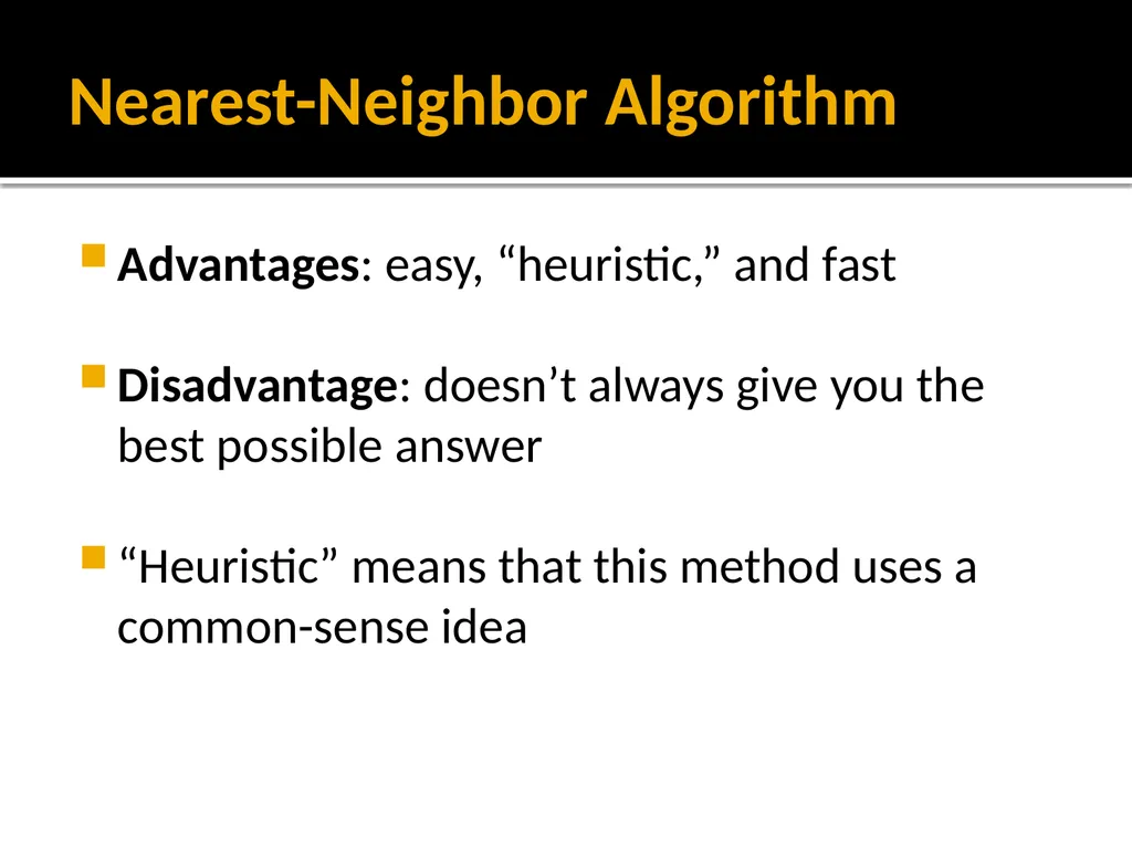
slide16. Nearest-Neighbor Algorithm Advantages: easy, “heuristic,” and fast
Disadvantage: doesn’t always give you the best possible answer
“Heuristic” means that this method uses a common-sense idea<br>
slide17. Sorted-Edges Algorithm Now let’s consider another algorithm for finding Hamiltonian circuits: the sorted-edges algorithm
This one is also based on a heuristic: use cheap edges before expensive ones<br>
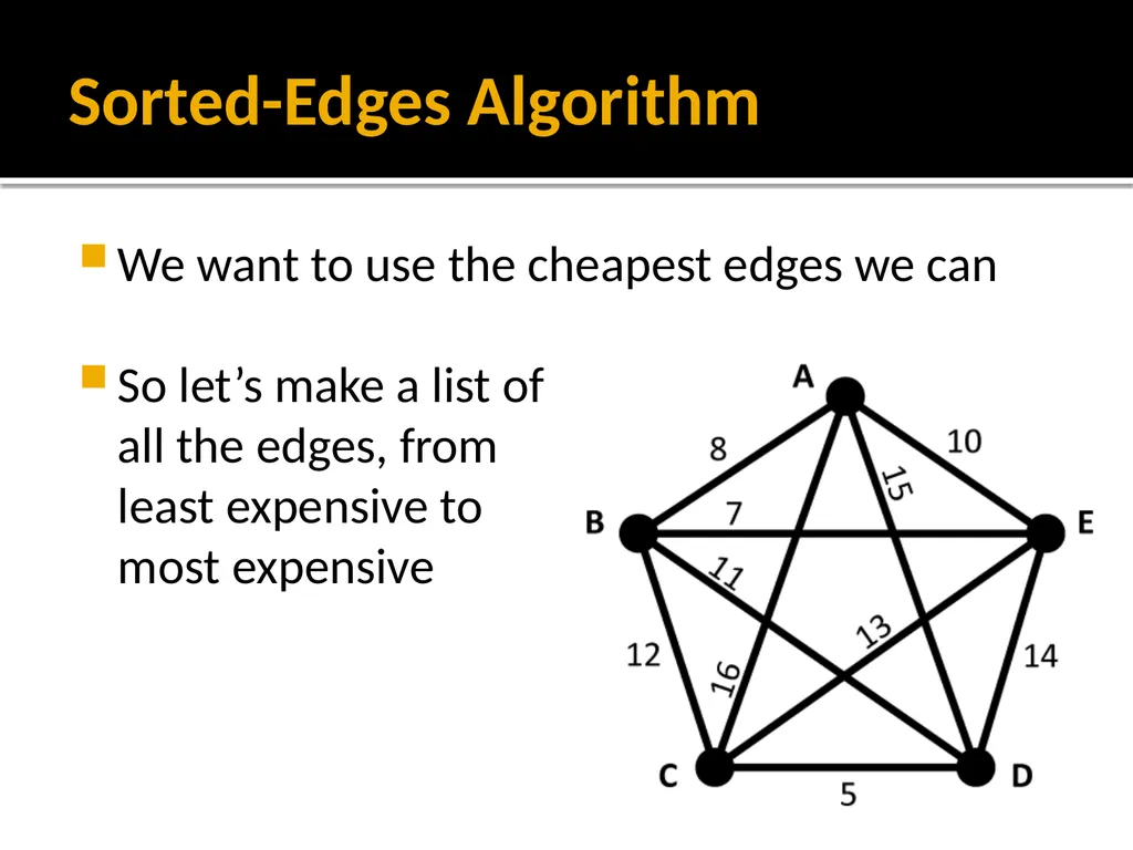
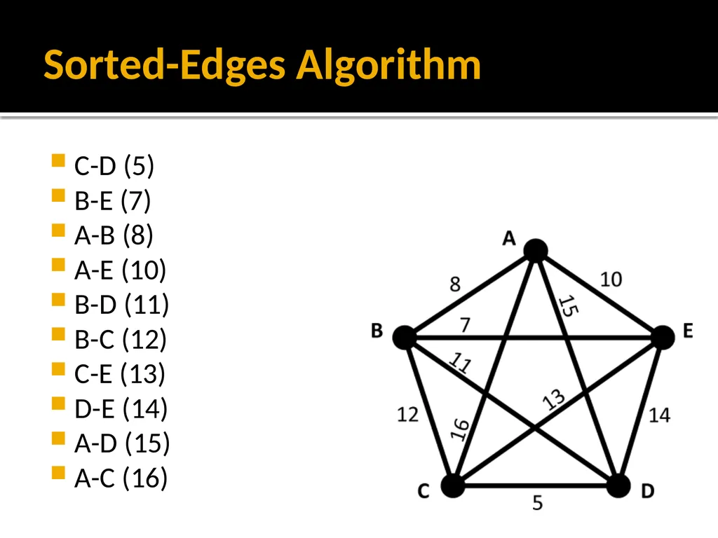
slide18. Sorted-Edges Algorithm We want to use the cheapest edges we can
So let’s make a list ofall the edges, from least expensive tomost expensive<br>
slide19. Sorted-Edges Algorithm C-D (5)
B-E (7)
A-B (8)
A-E (10)
B-D (11)
B-C (12)
C-E (13)
D-E (14)
A-D (15)
A-C (16)<br>
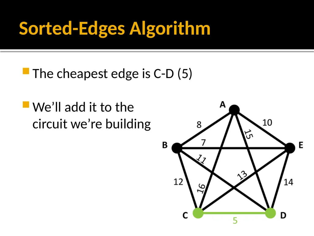
slide20. Sorted-Edges Algorithm The cheapest edge is C-D (5)
We’ll add it to thecircuit we’re building<br>
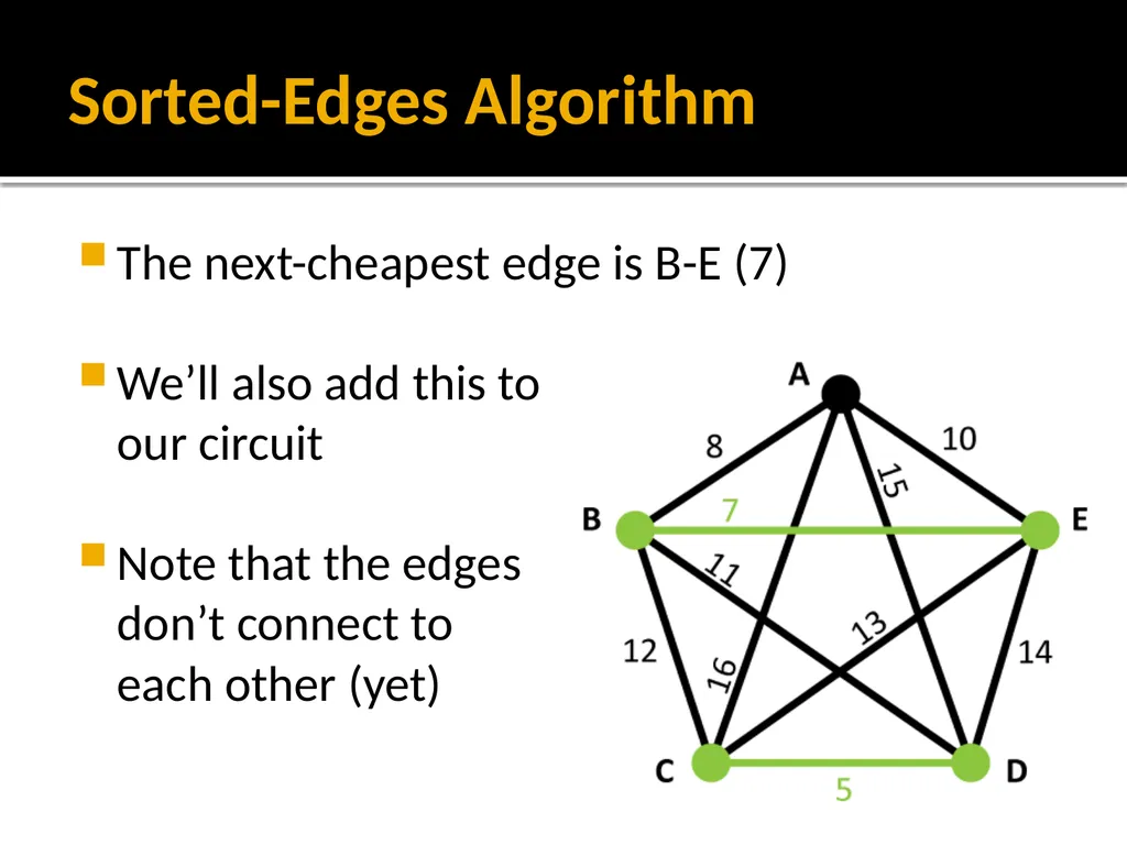
slide21. Sorted-Edges Algorithm The next-cheapest edge is B-E (7)
We’ll also add this toour circuit
Note that the edgesdon’t connect to each other (yet)<br>
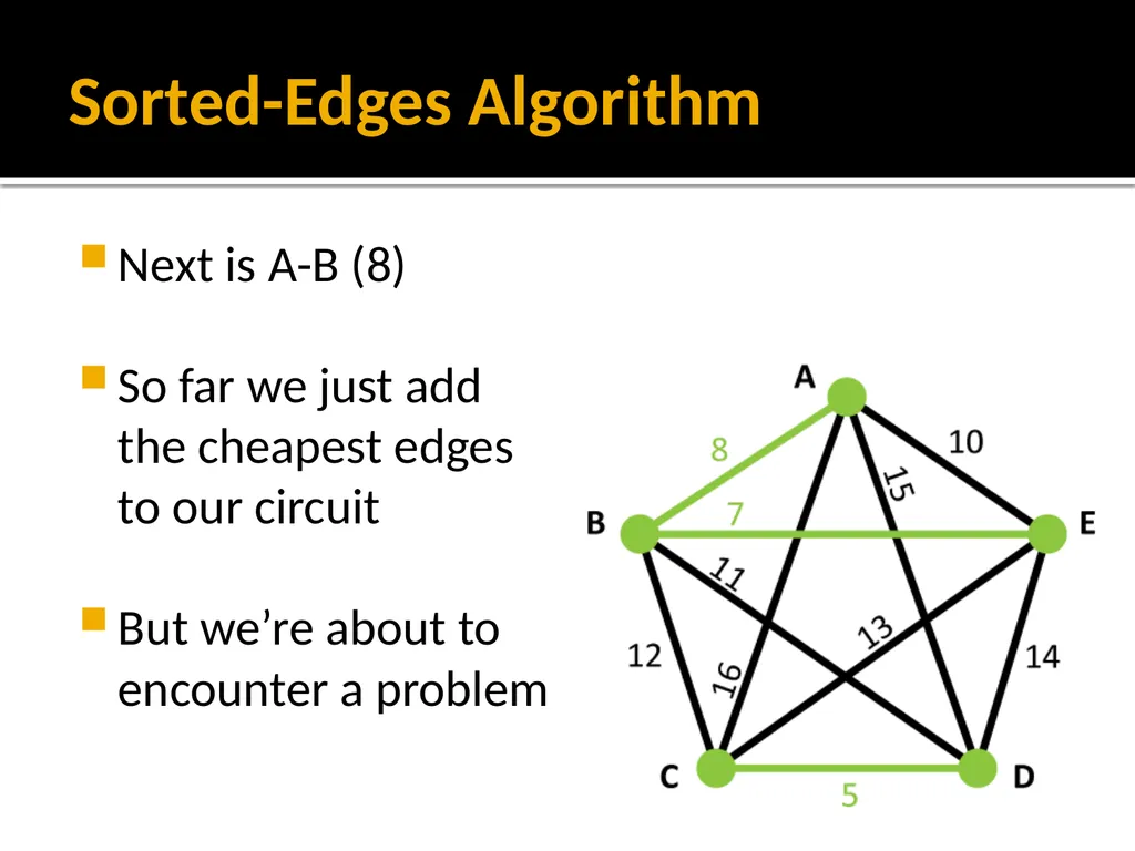
slide22. Sorted-Edges Algorithm Next is A-B (8)
So far we just addthe cheapest edgesto our circuit
But we’re about toencounter a problem<br>
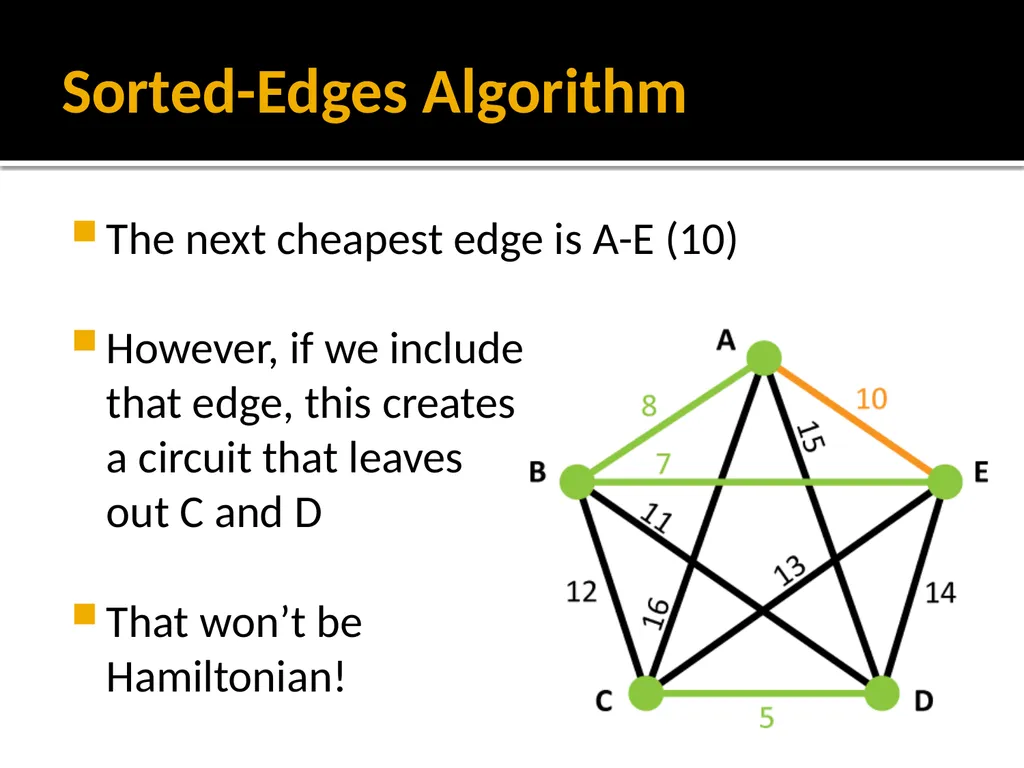
slide23. Sorted-Edges Algorithm The next cheapest edge is A-E (10)
However, if we includethat edge, this createsa circuit that leavesout C and D
That won’t be Hamiltonian!<br>
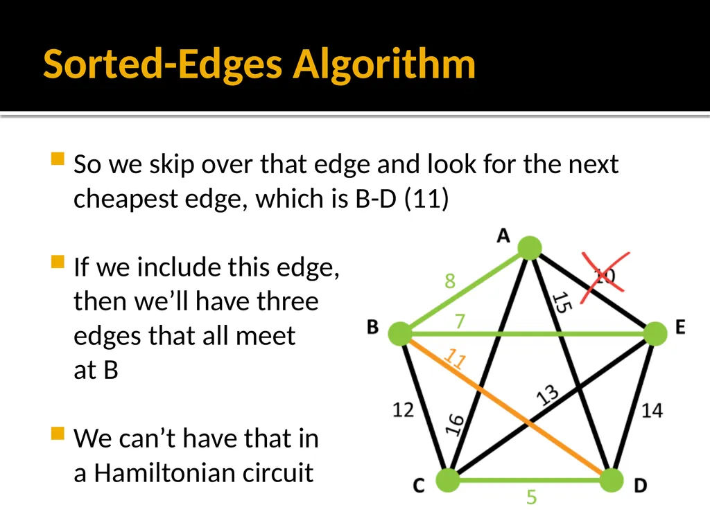
slide24. Sorted-Edges Algorithm So we skip over that edge and look for the next cheapest edge, which is B-D (11)
If we include this edge,then we’ll have threeedges that all meetat B
We can’t have that in a Hamiltonian circuit<br>
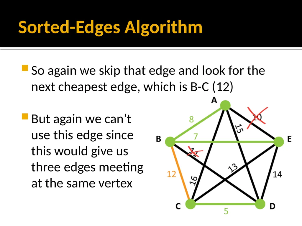
slide25. Sorted-Edges Algorithm So again we skip that edge and look for the next cheapest edge, which is B-C (12)
But again we can’tuse this edge sincethis would give usthree edges meetingat the same vertex<br>
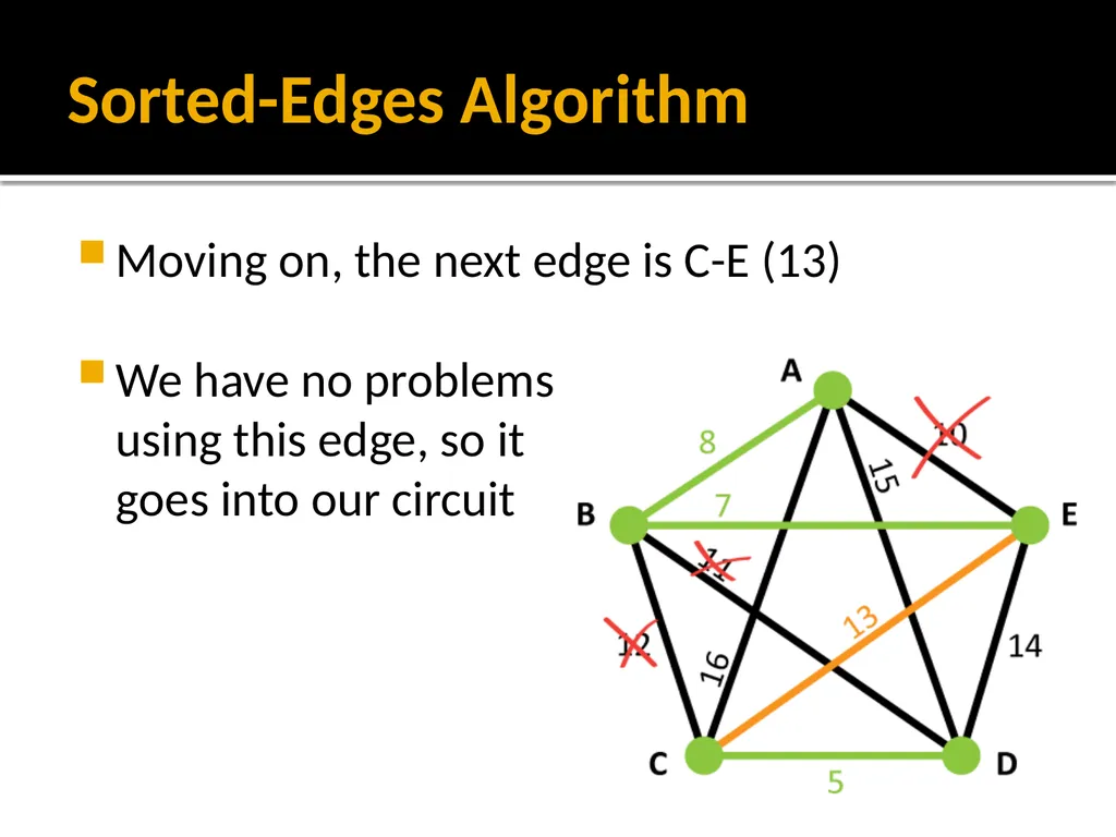
slide26. Sorted-Edges Algorithm Moving on, the next edge is C-E (13)
We have no problemsusing this edge, so itgoes into our circuit<br>
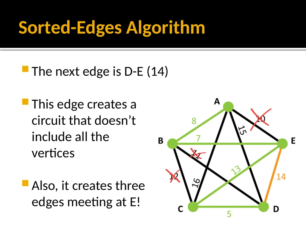
slide27. Sorted-Edges Algorithm The next edge is D-E (14)
This edge creates a circuit that doesn’tinclude all thevertices
Also, it creates threeedges meeting at E!<br>
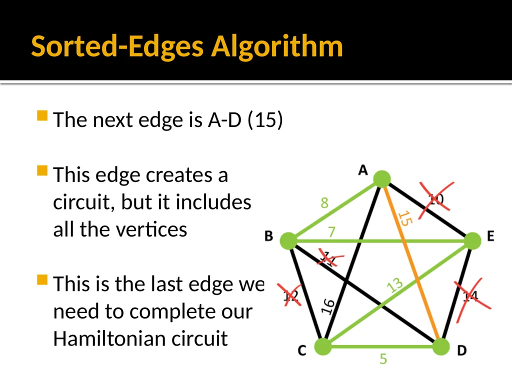
slide28. Sorted-Edges Algorithm The next edge is A-D (15)
This edge creates acircuit, but it includesall the vertices
This is the last edge weneed to complete ourHamiltonian circuit<br>
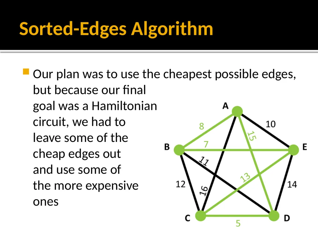
slide29. Sorted-Edges Algorithm Our plan was to use the cheapest possible edges, but because our finalgoal was a Hamiltoniancircuit, we had toleave some of thecheap edges out and use some of the more expensiveones<br>
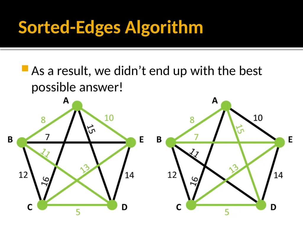
slide30. Sorted-Edges Algorithm As a result, we didn’t end up with the best possible answer!<br>
slide31. Sorted-Edges Algorithm Sort the edges from lowest cost to highest cost
Add edges to your circuit, one at a time, in order of increasing cost
Skip over edges that would cause you to have three edges at a single vertex or create a circuit that does not include all vertices
Keep going until you have a Hamiltonian circuit<br>
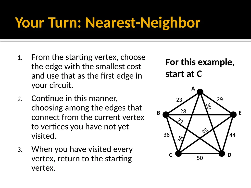
slide32. Your Turn: Nearest-Neighbor From the starting vertex, choose the edge with the smallest cost and use that as the first edge in your circuit.
Continue in this manner, choosing among the edges that connect from the current vertex to vertices you have not yet visited.
When you have visited every vertex, return to the starting vertex. For this example, start at C<br>
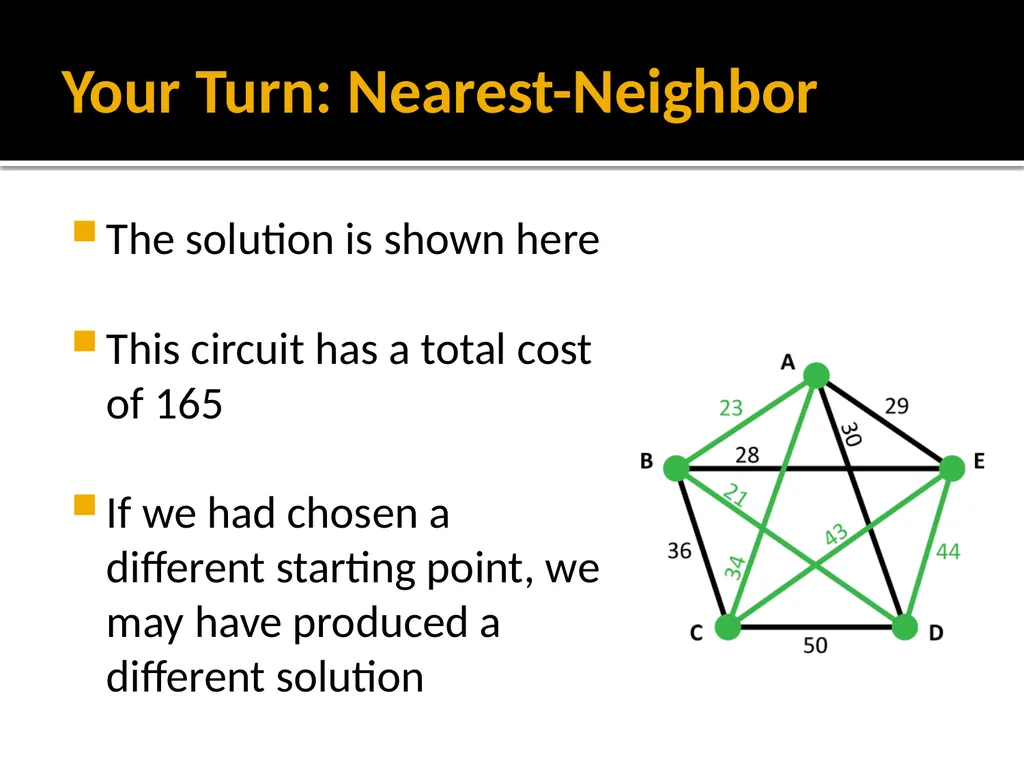
slide33. Your Turn: Nearest-Neighbor The solution is shown here
This circuit has a total cost of 165
If we had chosen a different starting point, we may have produced a different solution<br>
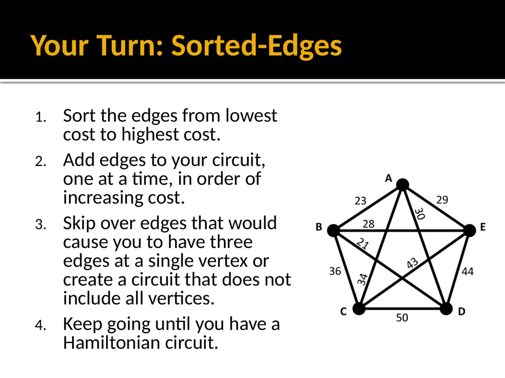
slide34. Your Turn: Sorted-Edges Sort the edges from lowest cost to highest cost.
Add edges to your circuit, one at a time, in order of increasing cost.
Skip over edges that would cause you to have three edges at a single vertex or create a circuit that does not include all vertices.
Keep going until you have a Hamiltonian circuit.<br>
slide35. Your Turn: Sorted-Edges The solution is shown here
This circuit has a total cost of 166
Did either method produce the best possible circuit? The only way to know for sure would be to use the brute-force method<br>

slide2. Brute Force is Hard! As we have seen, the brute force method can require us to examine a very large number of circuits
In this section we will develop algorithms for finding an answer much more quickly
The downside is that we will no longer be guaranteed to have the best possible answer<br>
slide3. Nearest-Neighbor Algorithm The first algorithm we will consider is called the nearest-neighbor algorithm
It’s based on a common sense idea: at each vertex, choose the closest vertex that you haven’t visited yet<br>

slide4. Nearest-Neighbor Algorithm We have to have a starting point
We will choose oursecond vertex byfinding the “nearestneighbor”<br>
slide5. Nearest-Neighbor Algorithm Where do we go first?
Choose the cheapest edge<br>
slide6. Nearest-Neighbor Algorithm Choose the cheapest edge
In this case, we gofrom B to E (7)<br>
slide7. Nearest-Neighbor Algorithm Now where do we go?
We can’t go backto B<br>
slide8. Nearest-Neighbor Algorithm Now where do we go?
We can’t go backto B
Again choose thecheapest edge<br>
slide9. Nearest-Neighbor Algorithm Now where do we go?
We can’t go backto E, but we alsocan’t go to B<br>
slide10. Nearest-Neighbor Algorithm The rule is “nearest neighbor”: always choose the lowest cost edge, unless that would take you back toa vertex you have already been to<br>
slide11. Nearest-Neighbor Algorithm Now we only have one choice
We can’t go back toA or E, and we can’treturn to B becausethat would leave out C<br>
slide12. Nearest-Neighbor Algorithm Now we only have one choice
We can’t go back toA or E, and we can’treturn to B becausethat would leave out C
So we must go to C<br>
slide13. Nearest-Neighbor Algorithm We have now visited all of the vertices, so we finally return to B
This circuit has a totalcost of 49
Is it the best circuit?<br>
slide14. Nearest-Neighbor Algorithm It is not the best! The solution on the left has a total cost of 47<br>
slide15. Nearest-Neighbor Algorithm From the starting vertex, choose the edge with the smallest cost and use that as the first edge in your circuit.
Continue in this manner, choosing among the edges that connect from the current vertex to vertices you have not yet visited.
When you have visited every vertex, return to the starting vertex.<br>
slide16. Nearest-Neighbor Algorithm Advantages: easy, “heuristic,” and fast
Disadvantage: doesn’t always give you the best possible answer
“Heuristic” means that this method uses a common-sense idea<br>
slide17. Sorted-Edges Algorithm Now let’s consider another algorithm for finding Hamiltonian circuits: the sorted-edges algorithm
This one is also based on a heuristic: use cheap edges before expensive ones<br>
slide18. Sorted-Edges Algorithm We want to use the cheapest edges we can
So let’s make a list ofall the edges, from least expensive tomost expensive<br>
slide19. Sorted-Edges Algorithm C-D (5)
B-E (7)
A-B (8)
A-E (10)
B-D (11)
B-C (12)
C-E (13)
D-E (14)
A-D (15)
A-C (16)<br>
slide20. Sorted-Edges Algorithm The cheapest edge is C-D (5)
We’ll add it to thecircuit we’re building<br>
slide21. Sorted-Edges Algorithm The next-cheapest edge is B-E (7)
We’ll also add this toour circuit
Note that the edgesdon’t connect to each other (yet)<br>
slide22. Sorted-Edges Algorithm Next is A-B (8)
So far we just addthe cheapest edgesto our circuit
But we’re about toencounter a problem<br>
slide23. Sorted-Edges Algorithm The next cheapest edge is A-E (10)
However, if we includethat edge, this createsa circuit that leavesout C and D
That won’t be Hamiltonian!<br>
slide24. Sorted-Edges Algorithm So we skip over that edge and look for the next cheapest edge, which is B-D (11)
If we include this edge,then we’ll have threeedges that all meetat B
We can’t have that in a Hamiltonian circuit<br>
slide25. Sorted-Edges Algorithm So again we skip that edge and look for the next cheapest edge, which is B-C (12)
But again we can’tuse this edge sincethis would give usthree edges meetingat the same vertex<br>
slide26. Sorted-Edges Algorithm Moving on, the next edge is C-E (13)
We have no problemsusing this edge, so itgoes into our circuit<br>
slide27. Sorted-Edges Algorithm The next edge is D-E (14)
This edge creates a circuit that doesn’tinclude all thevertices
Also, it creates threeedges meeting at E!<br>
slide28. Sorted-Edges Algorithm The next edge is A-D (15)
This edge creates acircuit, but it includesall the vertices
This is the last edge weneed to complete ourHamiltonian circuit<br>
slide29. Sorted-Edges Algorithm Our plan was to use the cheapest possible edges, but because our finalgoal was a Hamiltoniancircuit, we had toleave some of thecheap edges out and use some of the more expensiveones<br>
slide30. Sorted-Edges Algorithm As a result, we didn’t end up with the best possible answer!<br>
slide31. Sorted-Edges Algorithm Sort the edges from lowest cost to highest cost
Add edges to your circuit, one at a time, in order of increasing cost
Skip over edges that would cause you to have three edges at a single vertex or create a circuit that does not include all vertices
Keep going until you have a Hamiltonian circuit<br>
slide32. Your Turn: Nearest-Neighbor From the starting vertex, choose the edge with the smallest cost and use that as the first edge in your circuit.
Continue in this manner, choosing among the edges that connect from the current vertex to vertices you have not yet visited.
When you have visited every vertex, return to the starting vertex. For this example, start at C<br>
slide33. Your Turn: Nearest-Neighbor The solution is shown here
This circuit has a total cost of 165
If we had chosen a different starting point, we may have produced a different solution<br>
slide34. Your Turn: Sorted-Edges Sort the edges from lowest cost to highest cost.
Add edges to your circuit, one at a time, in order of increasing cost.
Skip over edges that would cause you to have three edges at a single vertex or create a circuit that does not include all vertices.
Keep going until you have a Hamiltonian circuit.<br>
slide35. Your Turn: Sorted-Edges The solution is shown here
This circuit has a total cost of 166
Did either method produce the best possible circuit? The only way to know for sure would be to use the brute-force method<br>