Slide 1 Mixed ANOVA (GLM 5) Prof. Andy Field Slide
Description: Slide 1 Mixed ANOVA (GLM 5) Prof. Andy Field Slide 2 Aims What is mixed ANOVA? Carrying out mixed ANOVA using R Interpretation Main effects Interactions Slide 3 What Is Three-Way Mixed ANOVA? Three independent variables Three-way 3 IVs
Related Topics
Download Presentation
"Slide 1 Mixed ANOVA (GLM 5) Prof. Andy Field Slide" is the property of its rightful owner. Permission is granted to download and print the materials on this website for personal, non-commercial use only, and to display it on your personal computer provided you do not modify the materials and that you retain all copyright notices contained in the materials. By downloading content from our website, you accept the terms of this agreement.
Presentation Transcript
slide1. Slide 1 Mixed ANOVA (GLM 5) Prof. Andy Field<br>
slide2. Slide 2 Aims What is mixed ANOVA?
Carrying out mixed ANOVA using R
Interpretation
Main effects
Interactions<br>
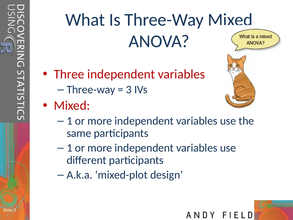
slide3. Slide 3 What Is Three-Way Mixed ANOVA? Three independent variables
Three-way = 3 IVs
Mixed:
1 or more independent variables use the same participants
1 or more independent variables use different participants
A.k.a. ‘mixed-plot design’<br>
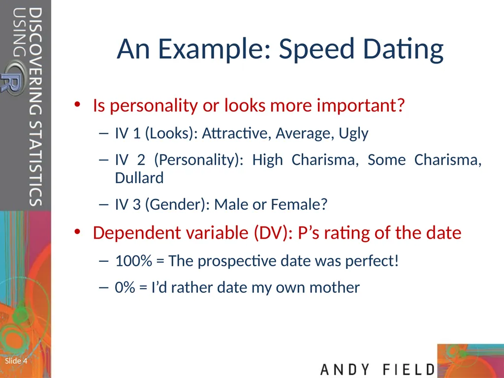
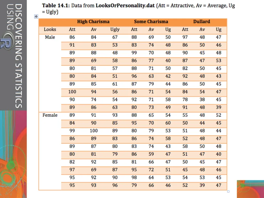
slide4. Slide 4 An Example: Speed Dating Is personality or looks more important?
IV 1 (Looks): Attractive, Average, Ugly
IV 2 (Personality): High Charisma, Some Charisma, Dullard
IV 3 (Gender): Male or Female?
Dependent variable (DV): P’s rating of the date
100% = The prospective date was perfect!
0% = I’d rather date my own mother<br>
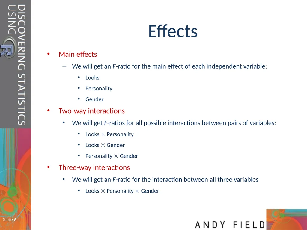
slide6. Slide 6 Effects Main effects
We will get an F-ratio for the main effect of each independent variable:
Looks
Personality
Gender
Two-way interactions
We will get F-ratios for all possible interactions between pairs of variables:
Looks Personality
Looks Gender
Personality Gender
Three-way interactions
We will get an F-ratio for the interaction between all three variables
Looks Personality Gender<br>
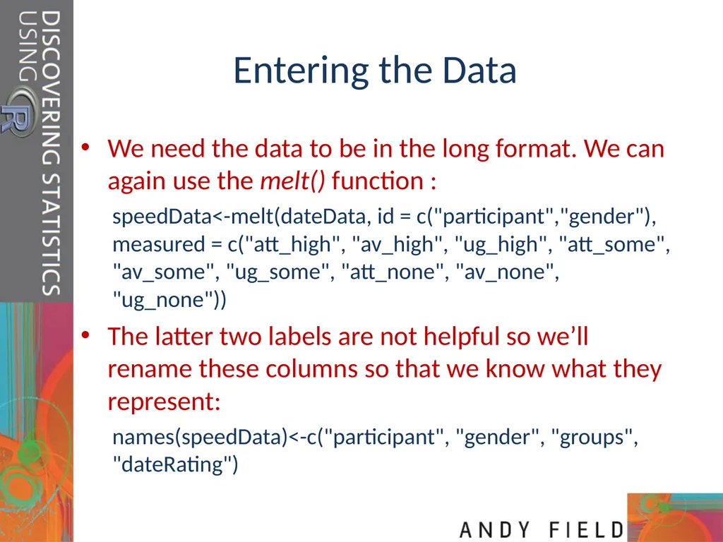
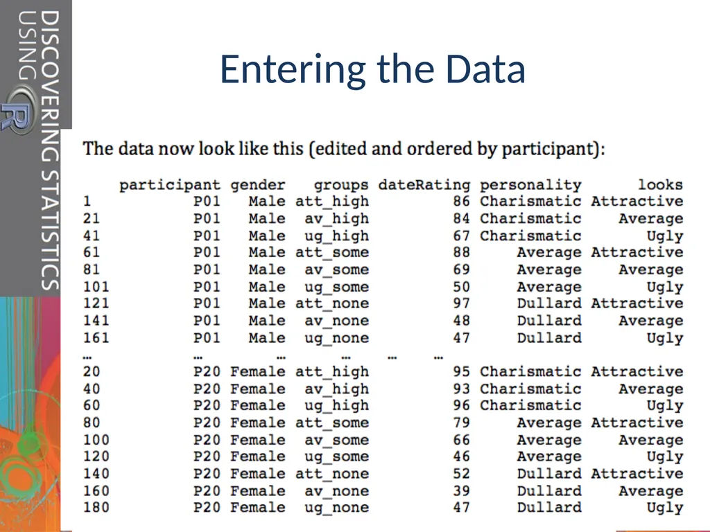
slide7. Entering the Data We need the data to be in the long format. We can again use the melt() function :
speedData<-melt(dateData, id = c("participant","gender"), measured = c("att_high", "av_high", "ug_high", "att_some", "av_some", "ug_some", "att_none", "av_none", "ug_none"))
The latter two labels are not helpful so we’ll rename these columns so that we know what they represent:
names(speedData)<-c("participant", "gender", "groups", "dateRating")<br>
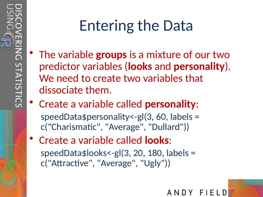
slide8. Entering the Data The variable groups is a mixture of our two predictor variables (looks and personality). We need to create two variables that dissociate them.
Create a variable called personality:
speedData$personality<-gl(3, 60, labels = c("Charismatic", "Average", "Dullard"))
Create a variable called looks:
speedData$looks<-gl(3, 20, 180, labels = c("Attractive", "Average", "Ugly"))<br>
slide9. Entering the Data<br>
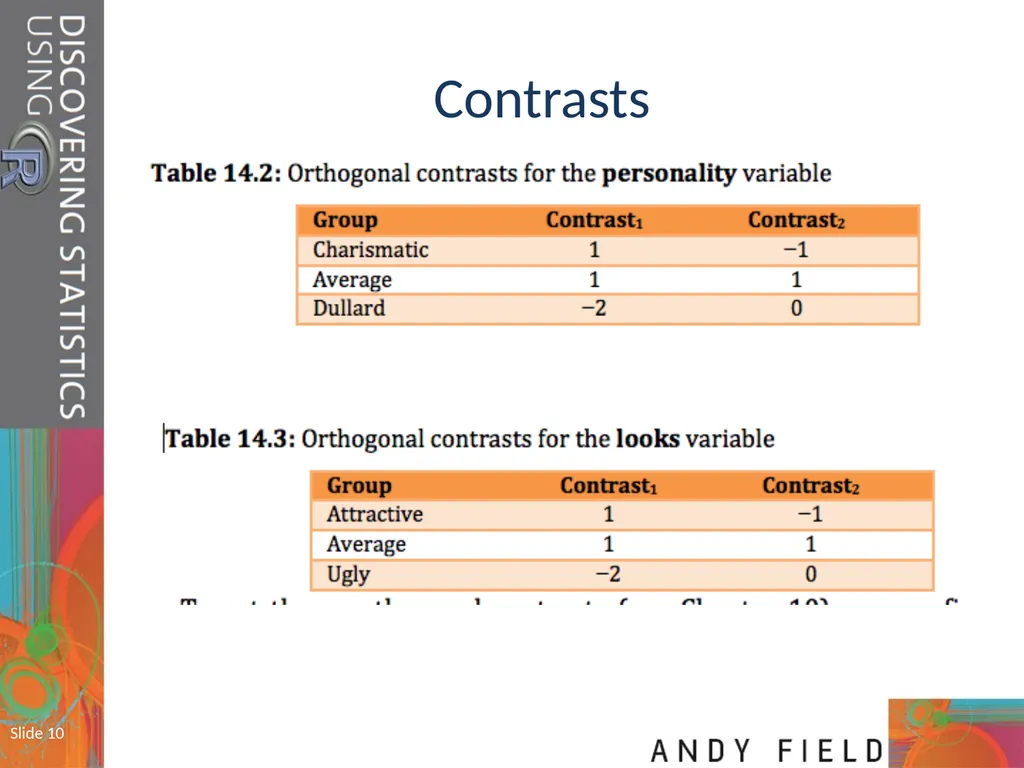
slide10. Slide 10 Contrasts<br>
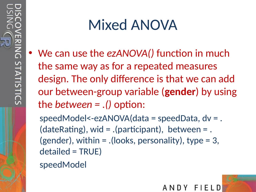
slide11. Mixed ANOVA We can use the ezANOVA() function in much the same way as for a repeated measures design. The only difference is that we can add our between-group variable (gender) by using the between = .() option:
speedModel<-ezANOVA(data = speedData, dv = .(dateRating), wid = .(participant), between = .(gender), within = .(looks, personality), type = 3, detailed = TRUE)
speedModel<br>
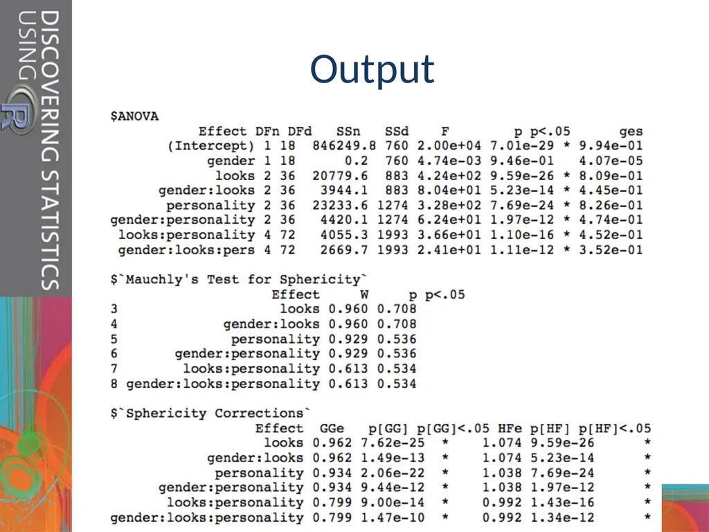
slide12. Output<br>
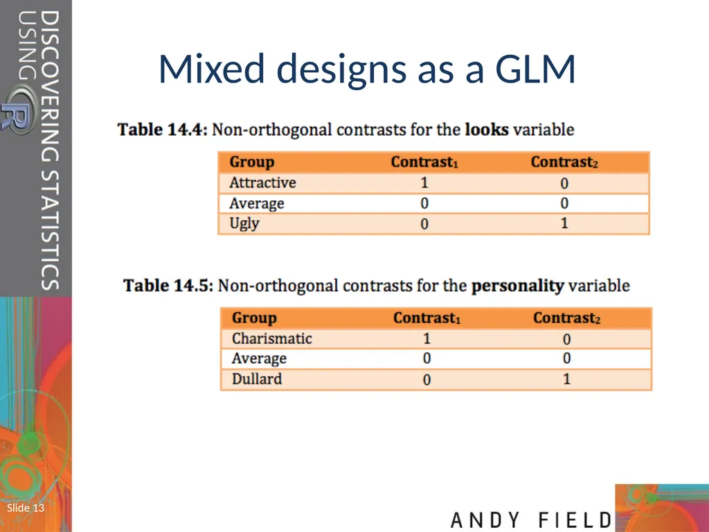
slide13. Slide 13 Mixed designs as a GLM<br>
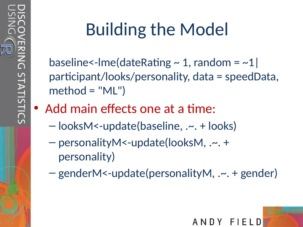
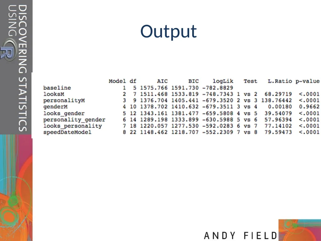
slide14. Building the Model baseline<-lme(dateRating ~ 1, random = ~1|participant/looks/personality, data = speedData, method = "ML")
Add main effects one at a time:
looksM<-update(baseline, .~. + looks)
personalityM<-update(looksM, .~. + personality)
genderM<-update(personalityM, .~. + gender)<br>
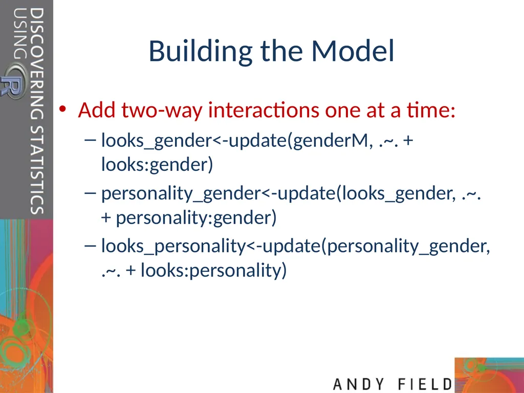
slide15. Building the Model Add two-way interactions one at a time:
looks_gender<-update(genderM, .~. + looks:gender)
personality_gender<-update(looks_gender, .~. + personality:gender)
looks_personality<-update(personality_gender, .~. + looks:personality)<br>
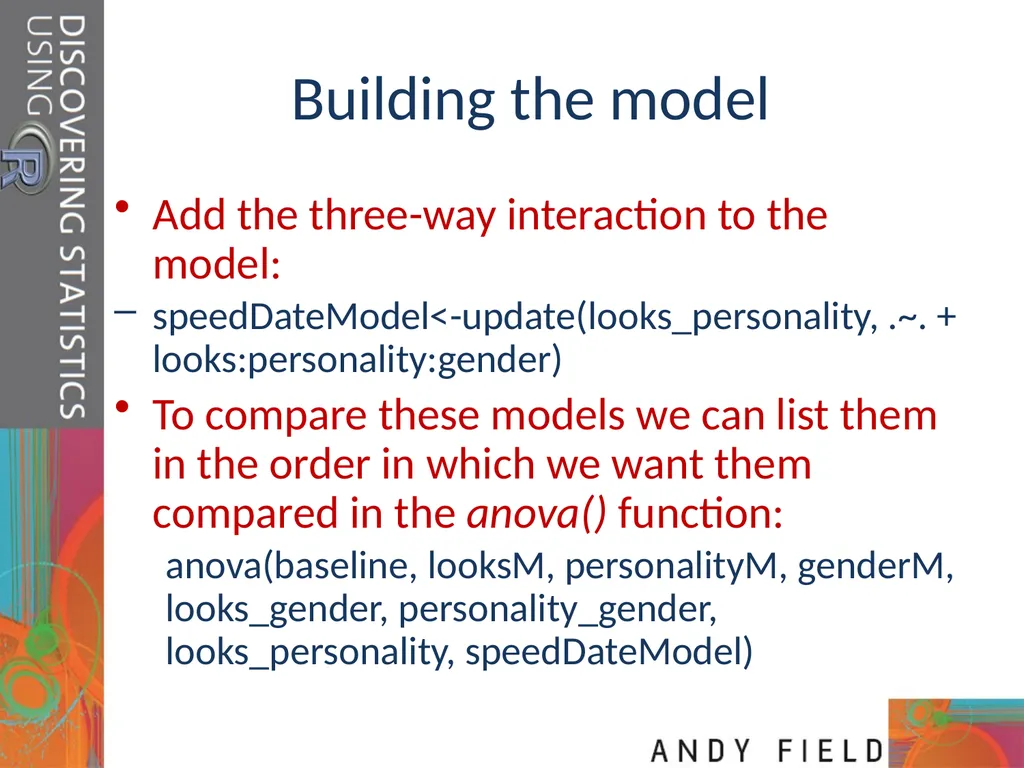
slide16. Building the model Add the three-way interaction to the model:
speedDateModel<-update(looks_personality, .~. + looks:personality:gender)
To compare these models we can list them in the order in which we want them compared in the anova() function:
anova(baseline, looksM, personalityM, genderM, looks_gender, personality_gender, looks_personality, speedDateModel)<br>

slide17. Output<br>
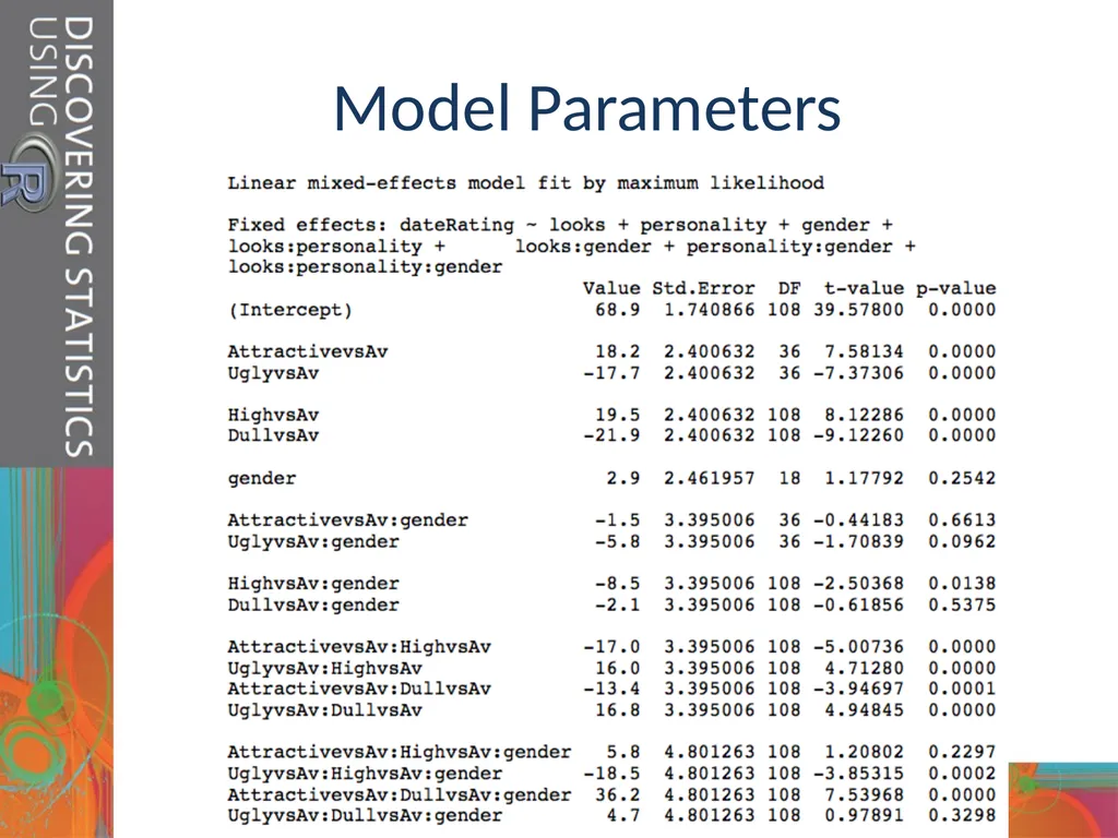
slide18. Model Parameters<br>
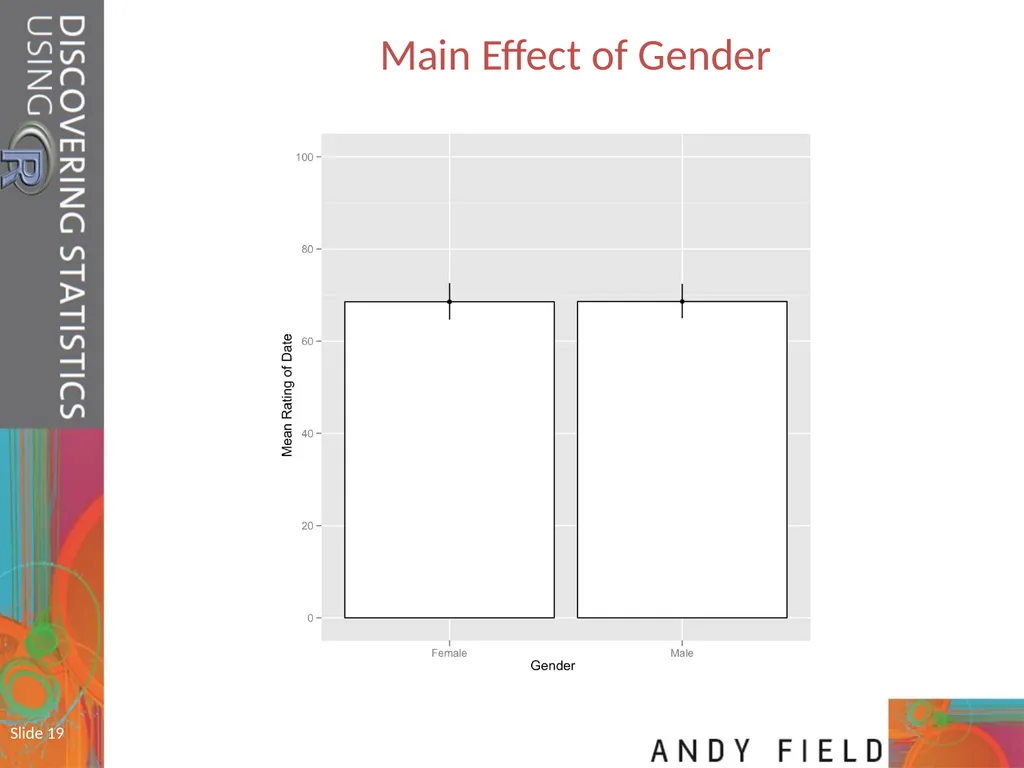
slide19. Slide 19 Main Effect of Gender<br>
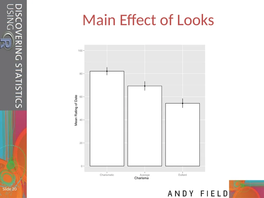
slide20. Slide 20 Main Effect of Looks<br>
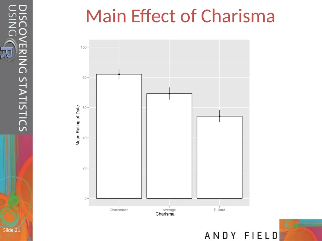
slide21. Slide 21 Main Effect of Charisma<br>
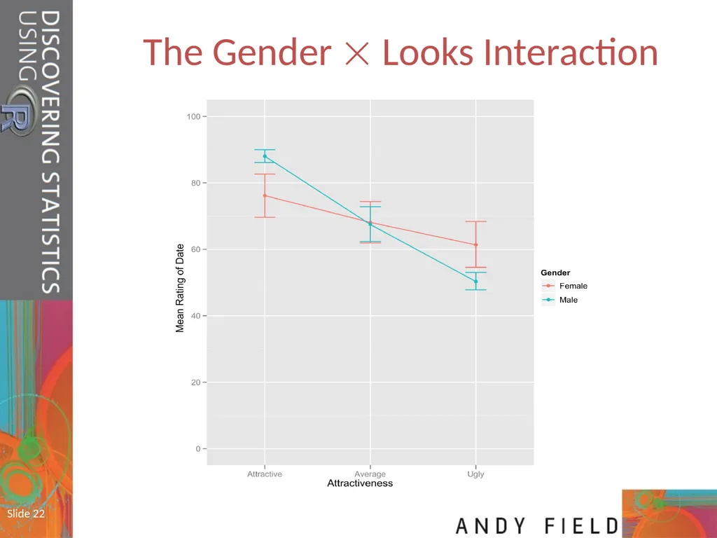
slide22. Slide 22 The Gender Looks Interaction<br>
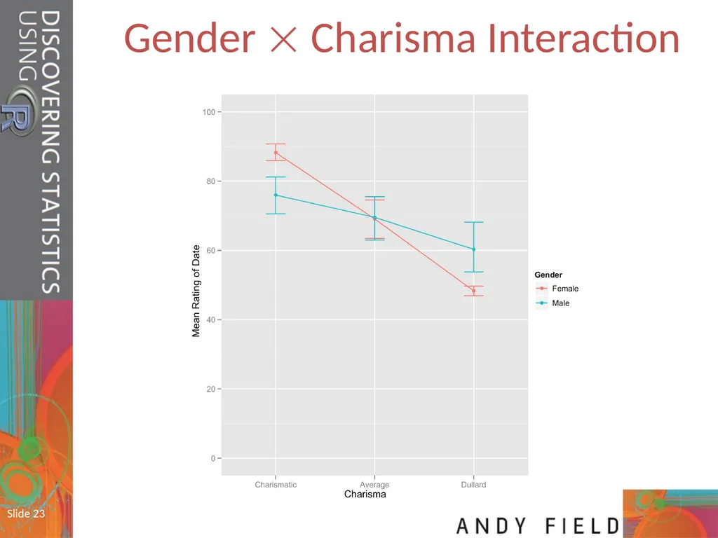
slide23. Slide 23 Gender Charisma Interaction<br>
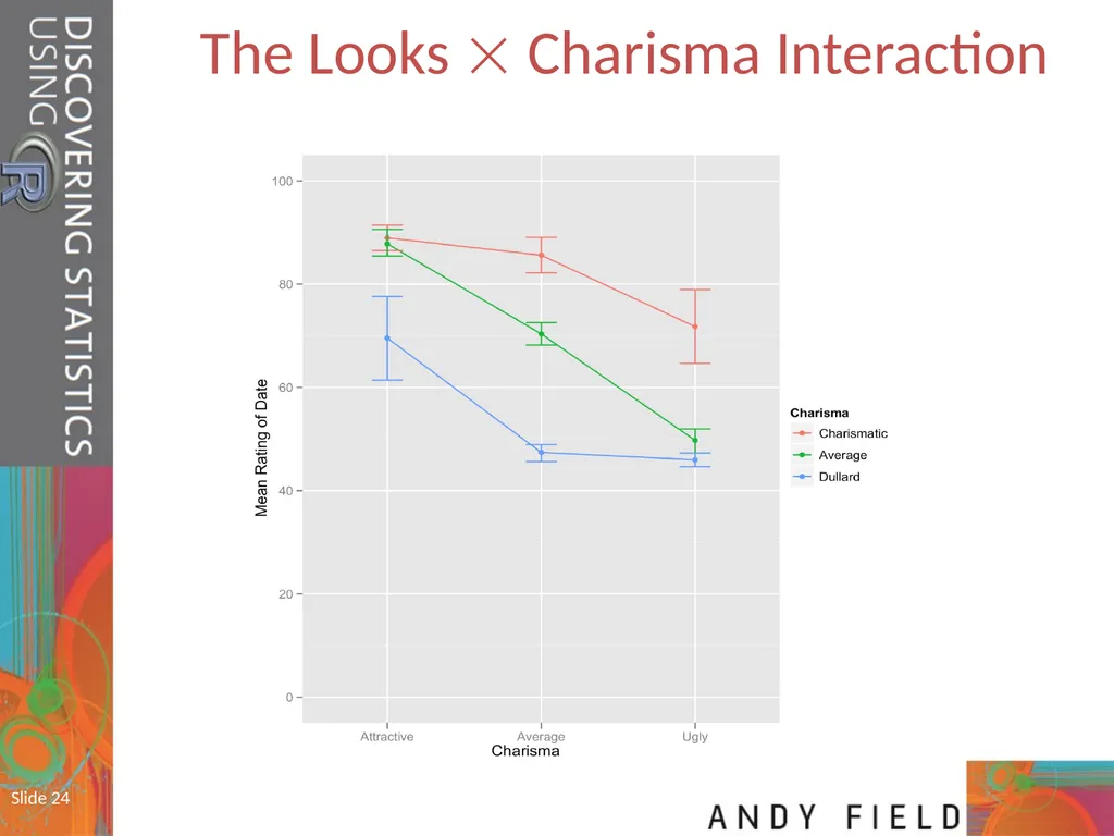
slide24. Slide 24 The Looks Charisma Interaction<br>
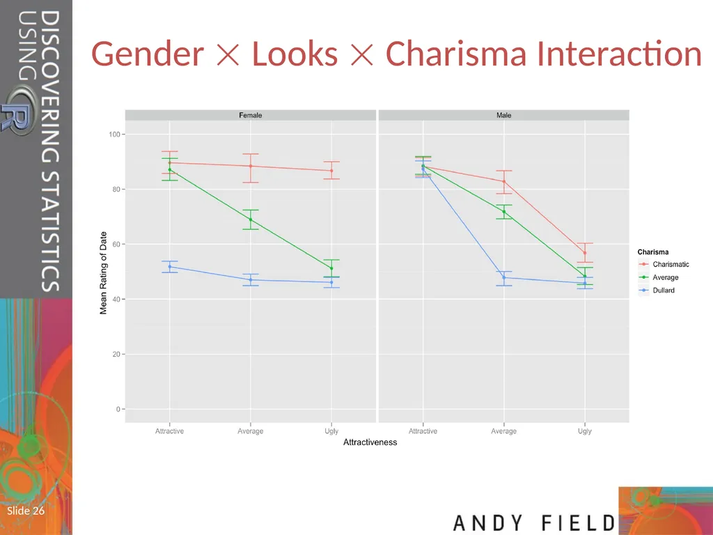
slide26. Slide 26 Gender Looks Charisma Interaction<br>
slide2. Slide 2 Aims What is mixed ANOVA?
Carrying out mixed ANOVA using R
Interpretation
Main effects
Interactions<br>
slide3. Slide 3 What Is Three-Way Mixed ANOVA? Three independent variables
Three-way = 3 IVs
Mixed:
1 or more independent variables use the same participants
1 or more independent variables use different participants
A.k.a. ‘mixed-plot design’<br>
slide4. Slide 4 An Example: Speed Dating Is personality or looks more important?
IV 1 (Looks): Attractive, Average, Ugly
IV 2 (Personality): High Charisma, Some Charisma, Dullard
IV 3 (Gender): Male or Female?
Dependent variable (DV): P’s rating of the date
100% = The prospective date was perfect!
0% = I’d rather date my own mother<br>
slide6. Slide 6 Effects Main effects
We will get an F-ratio for the main effect of each independent variable:
Looks
Personality
Gender
Two-way interactions
We will get F-ratios for all possible interactions between pairs of variables:
Looks Personality
Looks Gender
Personality Gender
Three-way interactions
We will get an F-ratio for the interaction between all three variables
Looks Personality Gender<br>
slide7. Entering the Data We need the data to be in the long format. We can again use the melt() function :
speedData<-melt(dateData, id = c("participant","gender"), measured = c("att_high", "av_high", "ug_high", "att_some", "av_some", "ug_some", "att_none", "av_none", "ug_none"))
The latter two labels are not helpful so we’ll rename these columns so that we know what they represent:
names(speedData)<-c("participant", "gender", "groups", "dateRating")<br>
slide8. Entering the Data The variable groups is a mixture of our two predictor variables (looks and personality). We need to create two variables that dissociate them.
Create a variable called personality:
speedData$personality<-gl(3, 60, labels = c("Charismatic", "Average", "Dullard"))
Create a variable called looks:
speedData$looks<-gl(3, 20, 180, labels = c("Attractive", "Average", "Ugly"))<br>
slide9. Entering the Data<br>
slide10. Slide 10 Contrasts<br>
slide11. Mixed ANOVA We can use the ezANOVA() function in much the same way as for a repeated measures design. The only difference is that we can add our between-group variable (gender) by using the between = .() option:
speedModel<-ezANOVA(data = speedData, dv = .(dateRating), wid = .(participant), between = .(gender), within = .(looks, personality), type = 3, detailed = TRUE)
speedModel<br>
slide12. Output<br>
slide13. Slide 13 Mixed designs as a GLM<br>
slide14. Building the Model baseline<-lme(dateRating ~ 1, random = ~1|participant/looks/personality, data = speedData, method = "ML")
Add main effects one at a time:
looksM<-update(baseline, .~. + looks)
personalityM<-update(looksM, .~. + personality)
genderM<-update(personalityM, .~. + gender)<br>
slide15. Building the Model Add two-way interactions one at a time:
looks_gender<-update(genderM, .~. + looks:gender)
personality_gender<-update(looks_gender, .~. + personality:gender)
looks_personality<-update(personality_gender, .~. + looks:personality)<br>
slide16. Building the model Add the three-way interaction to the model:
speedDateModel<-update(looks_personality, .~. + looks:personality:gender)
To compare these models we can list them in the order in which we want them compared in the anova() function:
anova(baseline, looksM, personalityM, genderM, looks_gender, personality_gender, looks_personality, speedDateModel)<br>
slide17. Output<br>
slide18. Model Parameters<br>
slide19. Slide 19 Main Effect of Gender<br>
slide20. Slide 20 Main Effect of Looks<br>
slide21. Slide 21 Main Effect of Charisma<br>
slide22. Slide 22 The Gender Looks Interaction<br>
slide23. Slide 23 Gender Charisma Interaction<br>
slide24. Slide 24 The Looks Charisma Interaction<br>
slide26. Slide 26 Gender Looks Charisma Interaction<br>