
Smoothing Techniques – A Primer Deepak Suyel
EM
Published · 49 slides · 0 views
1 / 1

Description
Smoothing Techniques A Primer Deepak Suyel Geetanjali Rakshit Sachin Pawar CS 626 Speech, NLP and the Web 02-Nov-12 1 Some terminology 2 Language Models Language models are useful for NLP applications such as Next word prediction
Related Topics
Share
Embed code
Download this presentation From Below
"Smoothing Techniques – A Primer Deepak Suyel" is the property of its rightful owner. Permission is granted to download and print the materials on this website for personal, non-commercial use only, and to display it on your personal computer provided you do not modify the materials and that you retain all copyright notices contained in the materials. By downloading content from our website, you accept the terms of this agreement.
Presentation Transcript
01
Smoothing Techniques – A Primer Deepak Suyel
Geetanjali Rakshit
Sachin Pawar CS 626 – Speech, NLP and the Web 02-Nov-12 1<br>
Geetanjali Rakshit
Sachin Pawar CS 626 – Speech, NLP and the Web 02-Nov-12 1<br>
02
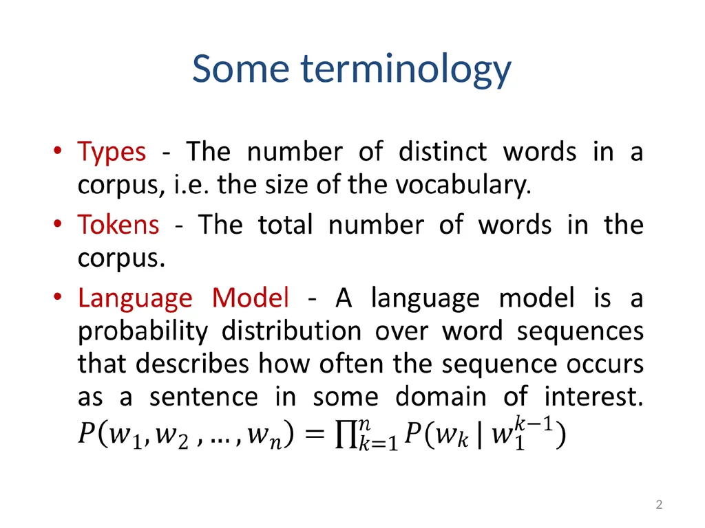
Some terminology 2<br>
03
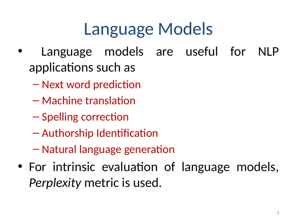
Language Models Language models are useful for NLP applications such as
Next word prediction
Machine translation
Spelling correction
Authorship Identification
Natural language generation
For intrinsic evaluation of language models, Perplexity metric is used. 3<br>
Next word prediction
Machine translation
Spelling correction
Authorship Identification
Natural language generation
For intrinsic evaluation of language models, Perplexity metric is used. 3<br>
04
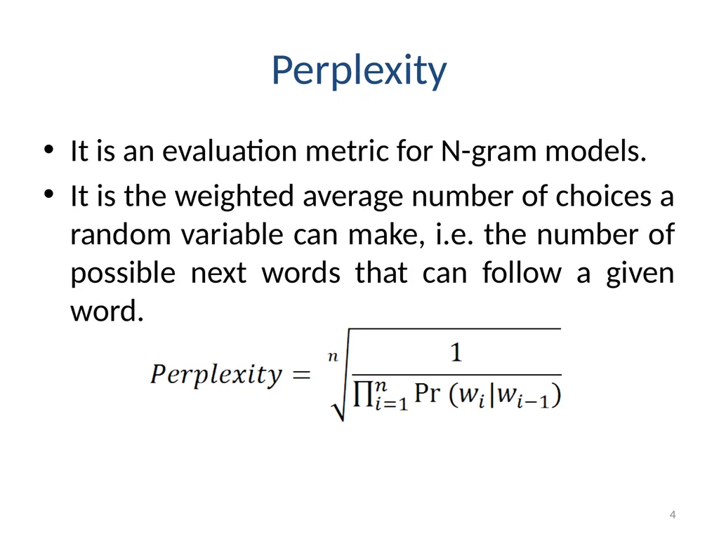
Perplexity It is an evaluation metric for N-gram models.
It is the weighted average number of choices a random variable can make, i.e. the number of possible next words that can follow a given word. 4<br>
It is the weighted average number of choices a random variable can make, i.e. the number of possible next words that can follow a given word. 4<br>
05
Roadmap Motivation
Types of smoothing
Back-off
Interpolation
Comparison of smoothing techniques 5<br>
Types of smoothing
Back-off
Interpolation
Comparison of smoothing techniques 5<br>
06
The Berkeley Restaurant Example Corpora
Can you tell me about any good cantonese restaurants close by
Mid-priced Thai food is what I’m looking for
Can you give me a listing of the kinds of food that are available
I am looking for a good place to eat breakfast 6<br>
Can you tell me about any good cantonese restaurants close by
Mid-priced Thai food is what I’m looking for
Can you give me a listing of the kinds of food that are available
I am looking for a good place to eat breakfast 6<br>
07
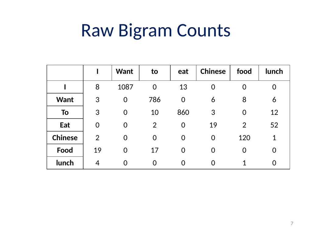
Raw Bigram Counts 7<br>
08
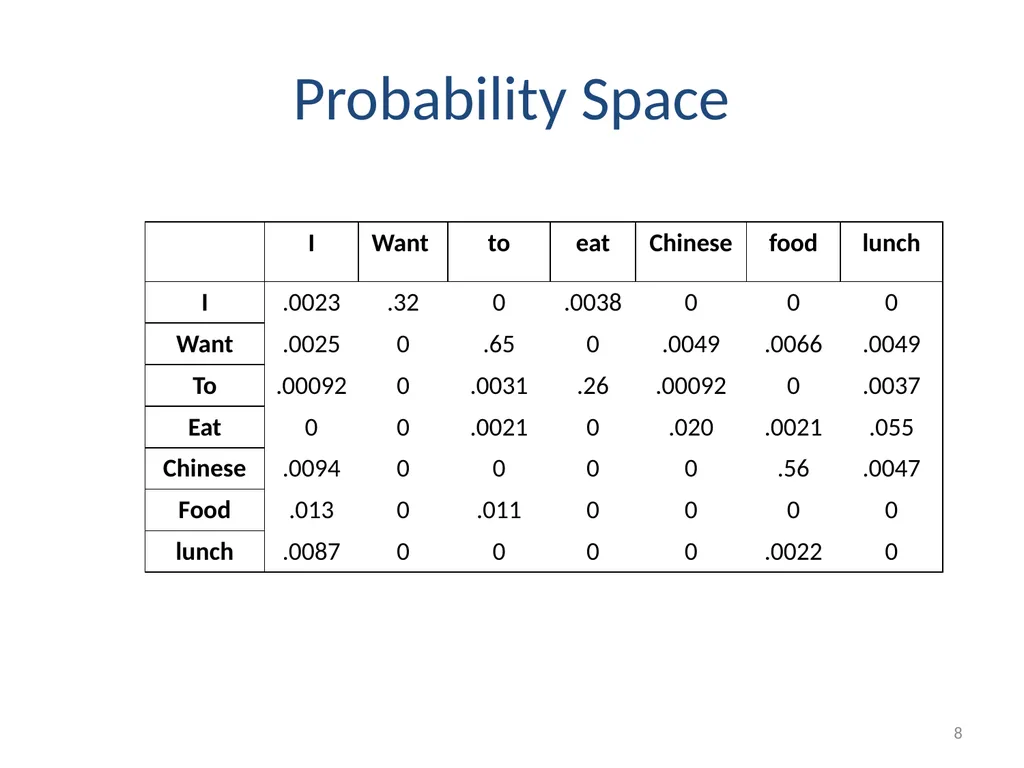
Probability Space 8<br>
09
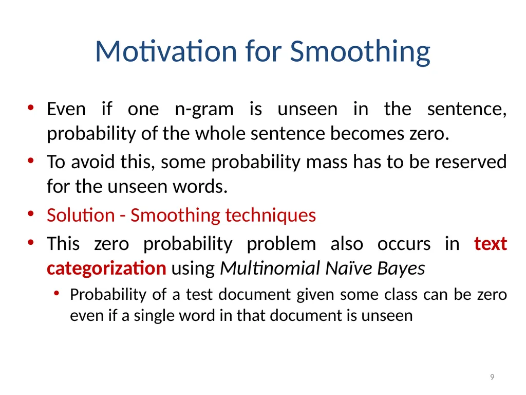
Motivation for Smoothing Even if one n-gram is unseen in the sentence, probability of the whole sentence becomes zero.
To avoid this, some probability mass has to be reserved for the unseen words.
Solution - Smoothing techniques
This zero probability problem also occurs in text categorization using Multinomial Naïve Bayes
Probability of a test document given some class can be zero even if a single word in that document is unseen 9<br>
10
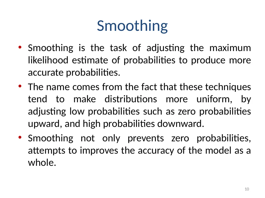
Smoothing Smoothing is the task of adjusting the maximum likelihood estimate of probabilities to produce more accurate probabilities.
The name comes from the fact that these techniques tend to make distributions more uniform, by adjusting low probabilities such as zero probabilities upward, and high probabilities downward.
Smoothing not only prevents zero probabilities, attempts to improves the accuracy of the model as a whole. 10<br>
11
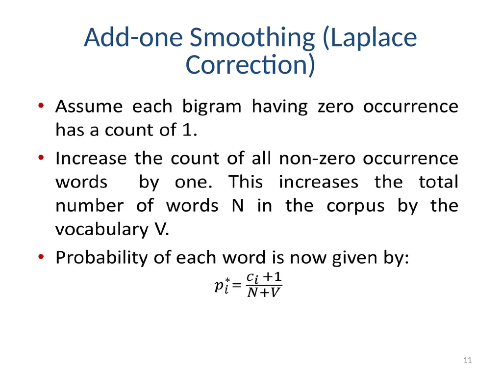
Add-one Smoothing (Laplace Correction) 11<br>
12
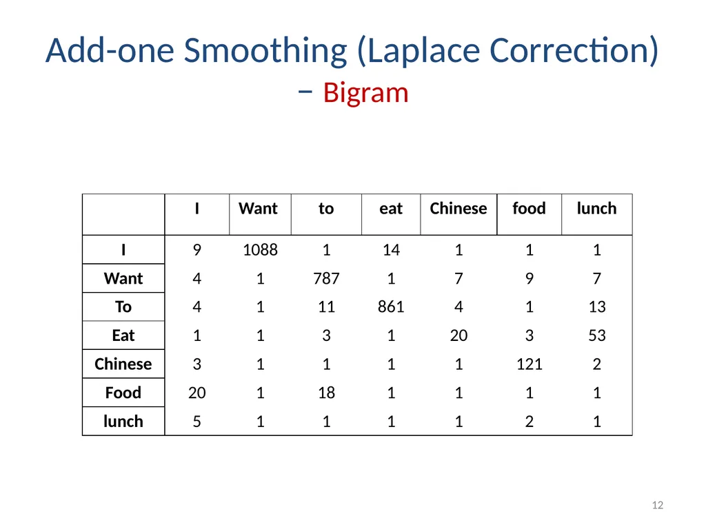
Add-one Smoothing (Laplace Correction) – Bigram 12<br>
13
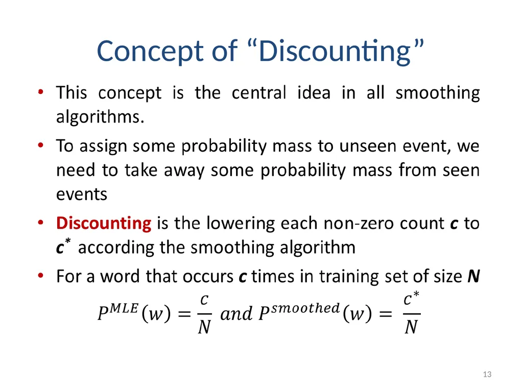
Concept of “Discounting” 13<br>
14
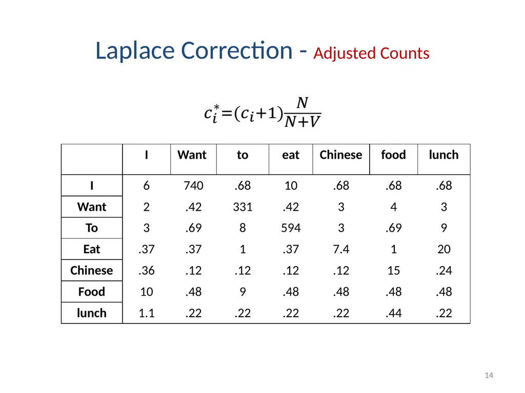
Laplace Correction - Adjusted Counts 14<br>
15
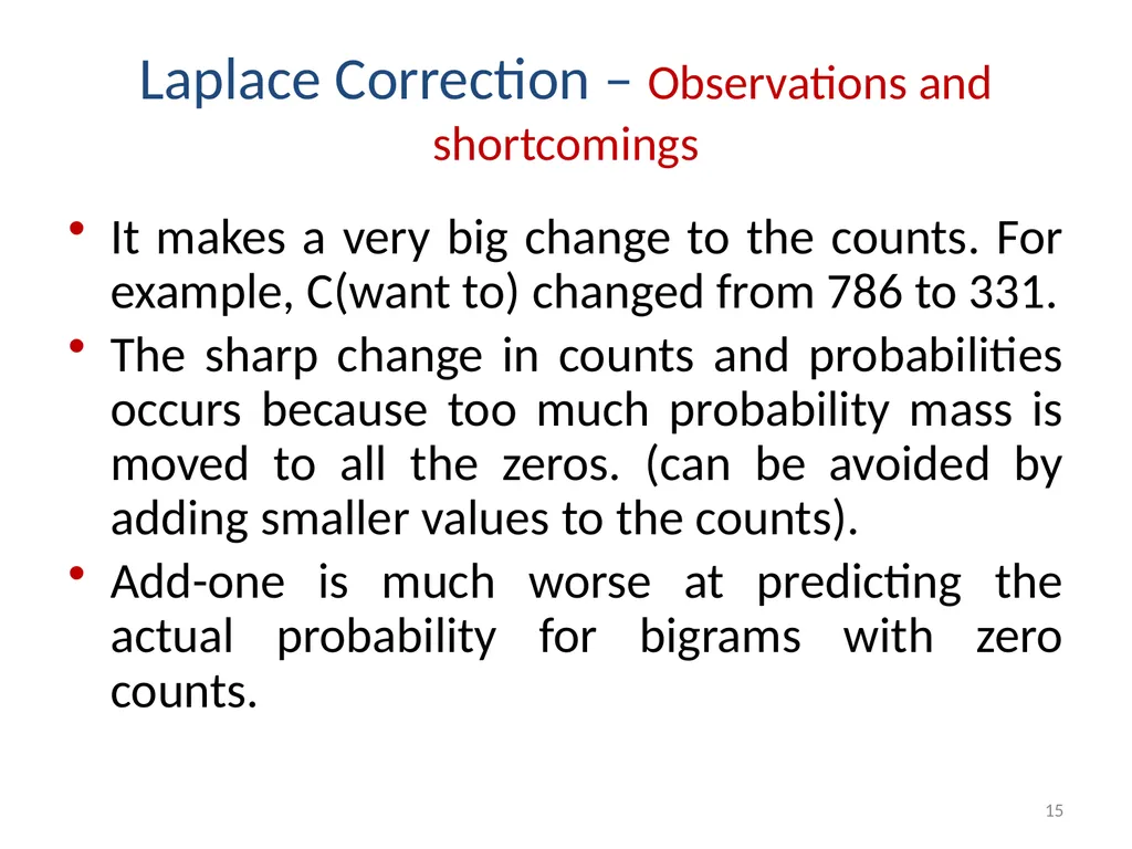
Laplace Correction – Observations and shortcomings It makes a very big change to the counts. For example, C(want to) changed from 786 to 331.
The sharp change in counts and probabilities occurs because too much probability mass is moved to all the zeros. (can be avoided by adding smaller values to the counts).
Add-one is much worse at predicting the actual probability for bigrams with zero counts. 15<br>
The sharp change in counts and probabilities occurs because too much probability mass is moved to all the zeros. (can be avoided by adding smaller values to the counts).
Add-one is much worse at predicting the actual probability for bigrams with zero counts. 15<br>
16
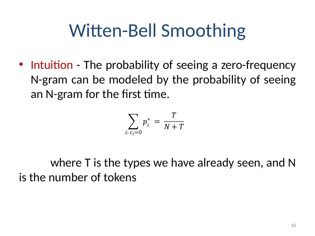
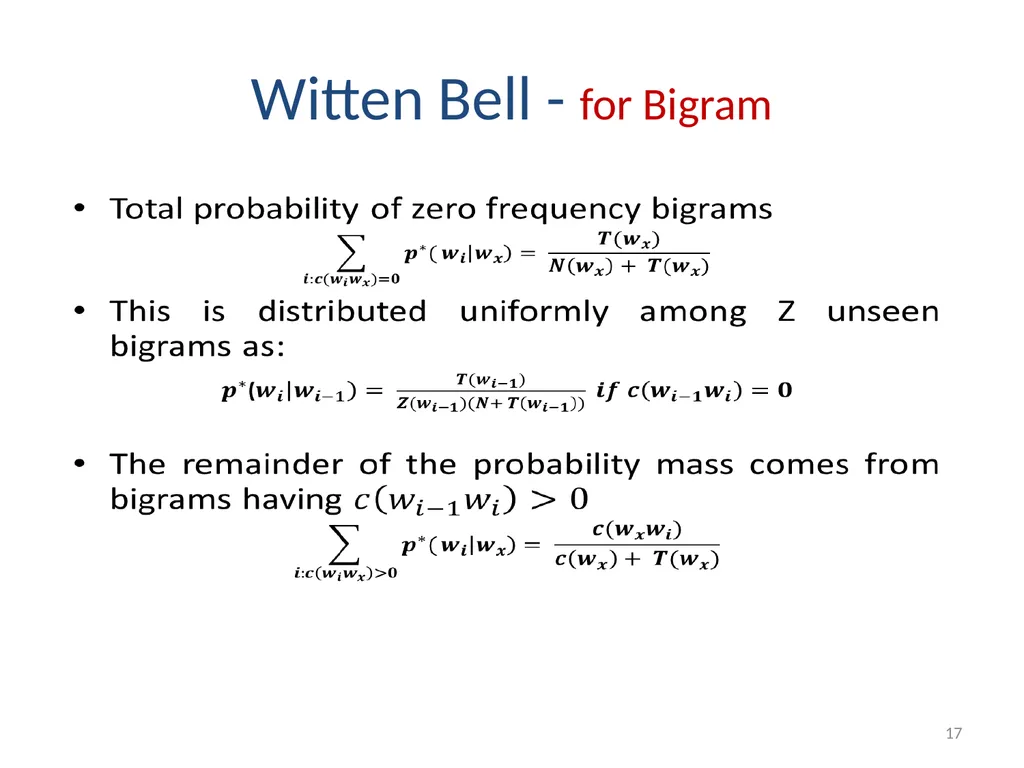
Witten-Bell Smoothing Intuition - The probability of seeing a zero-frequency N-gram can be modeled by the probability of seeing an N-gram for the first time.
where T is the types we have already seen, and N is the number of tokens 16<br>
where T is the types we have already seen, and N is the number of tokens 16<br>
17
Witten Bell - for Bigram 17<br>
18
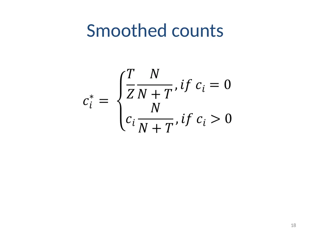
Smoothed counts 18<br>
19
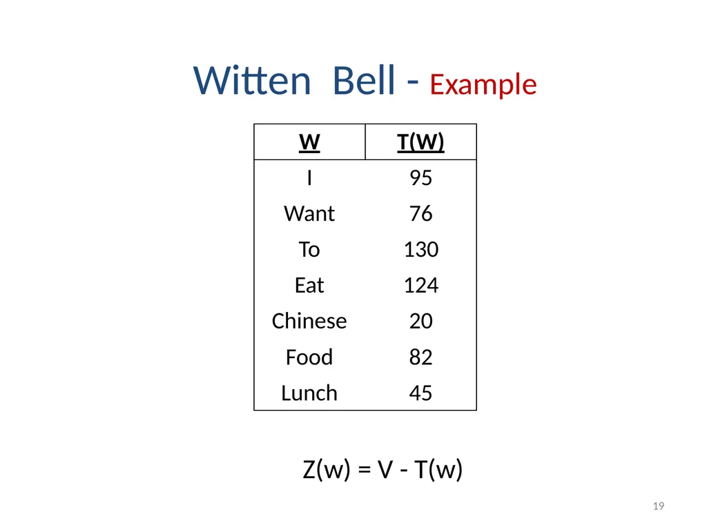
19 Witten Bell - Example Z(w) = V - T(w)<br>
20
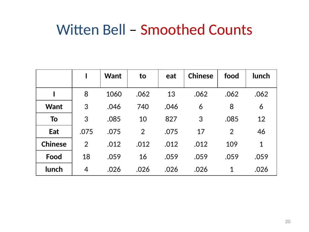
Witten Bell – Smoothed Counts 20<br>
21
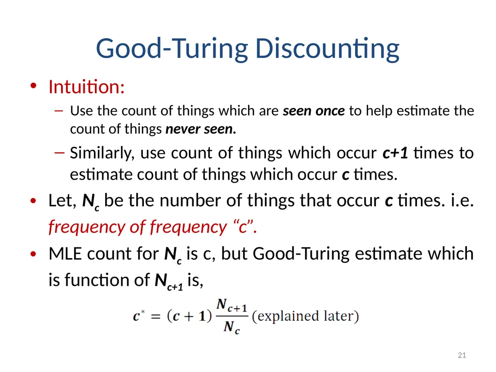
Good-Turing Discounting Intuition:
Use the count of things which are seen once to help estimate the count of things never seen.
Similarly, use count of things which occur c+1 times to estimate count of things which occur c times.
Let, Nc be the number of things that occur c times. i.e. frequency of frequency “c”.
MLE count for Nc is c, but Good-Turing estimate which is function of Nc+1 is, 21<br>
22
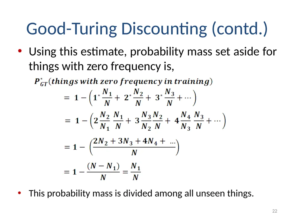
Good-Turing Discounting (contd.) Using this estimate, probability mass set aside for things with zero frequency is,
This probability mass is divided among all unseen things. 22<br>
This probability mass is divided among all unseen things. 22<br>
23
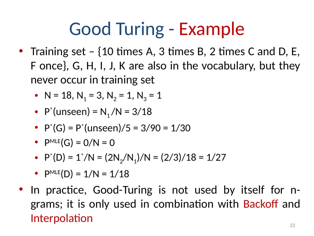
Good Turing - Example Training set – {10 times A, 3 times B, 2 times C and D, E, F once}, G, H, I, J, K are also in the vocabulary, but they never occur in training set
N = 18, N1 = 3, N2 = 1, N3 = 1
P*(unseen) = N1 /N = 3/18
P*(G) = P*(unseen)/5 = 3/90 = 1/30
PMLE(G) = 0/N = 0
P*(D) = 1*/N = (2N2/N1)/N = (2/3)/18 = 1/27
PMLE(D) = 1/N = 1/18
In practice, Good-Turing is not used by itself for n-grams; it is only used in combination with Backoff and Interpolation 23<br>
24
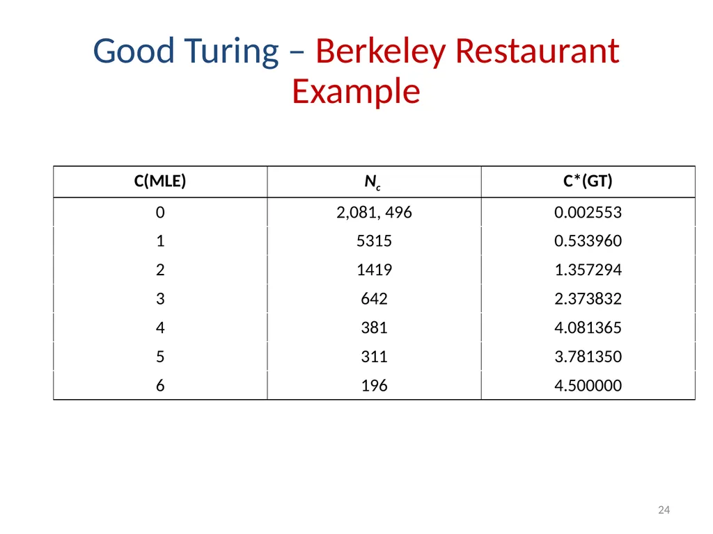
Good Turing – Berkeley Restaurant Example 24<br>
25
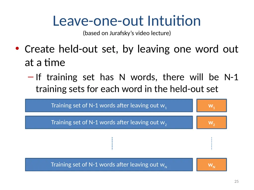
Leave-one-out Intuition
(based on Jurafsky’s video lecture) Create held-out set, by leaving one word out at a time
If training set has N words, there will be N-1 training sets for each word in the held-out set Training set of N-1 words after leaving out w1 w1 Training set of N-1 words after leaving out w2 w2 Training set of N-1 words after leaving out wN wN 25<br>
If training set has N words, there will be N-1 training sets for each word in the held-out set Training set of N-1 words after leaving out w1 w1 Training set of N-1 words after leaving out w2 w2 Training set of N-1 words after leaving out wN wN 25<br>
26
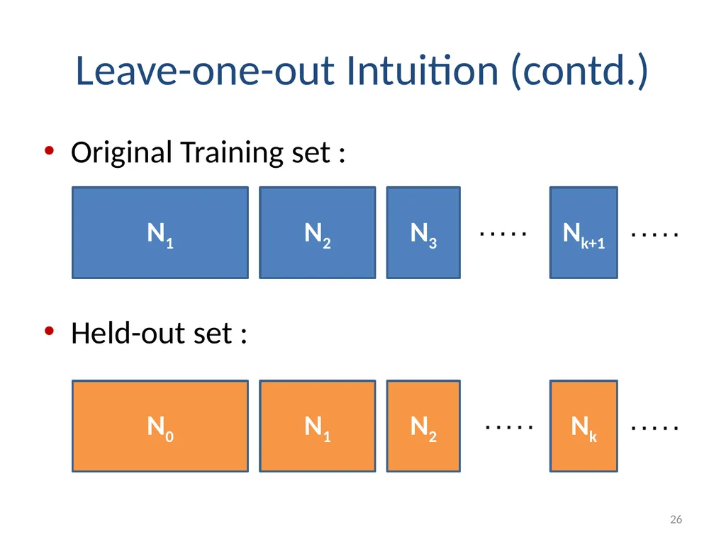
Leave-one-out Intuition (contd.) Original Training set :
Held-out set : N1 N2 N3 Nk+1 N0 N1 N2 Nk 26<br>
Held-out set : N1 N2 N3 Nk+1 N0 N1 N2 Nk 26<br>
27
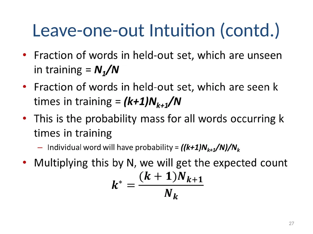
Leave-one-out Intuition (contd.) 27<br>
28
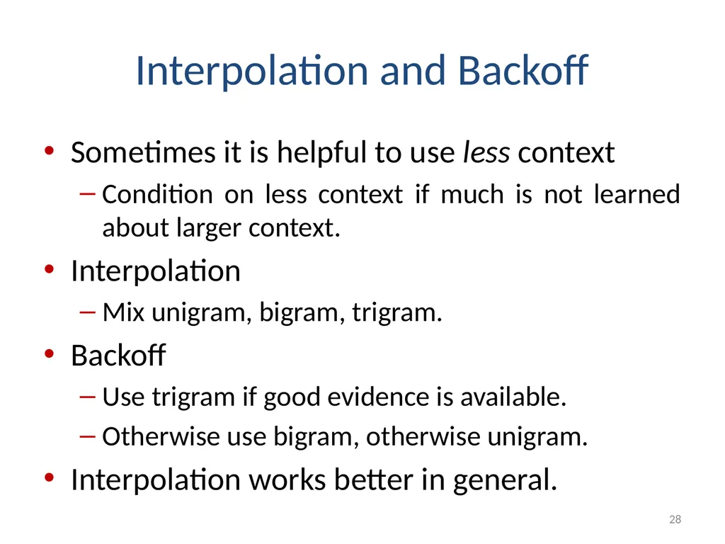
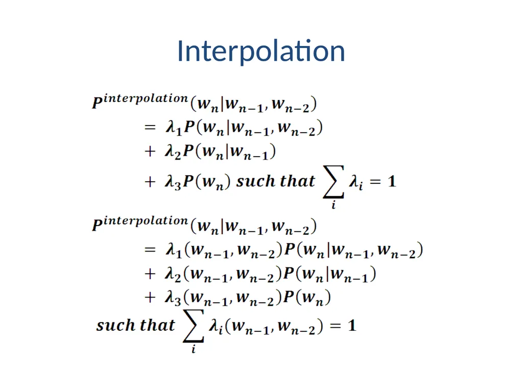
Interpolation and Backoff Sometimes it is helpful to use less context
Condition on less context if much is not learned about larger context.
Interpolation
Mix unigram, bigram, trigram.
Backoff
Use trigram if good evidence is available.
Otherwise use bigram, otherwise unigram.
Interpolation works better in general. 28<br>
Condition on less context if much is not learned about larger context.
Interpolation
Mix unigram, bigram, trigram.
Backoff
Use trigram if good evidence is available.
Otherwise use bigram, otherwise unigram.
Interpolation works better in general. 28<br>
29
Interpolation<br>
30
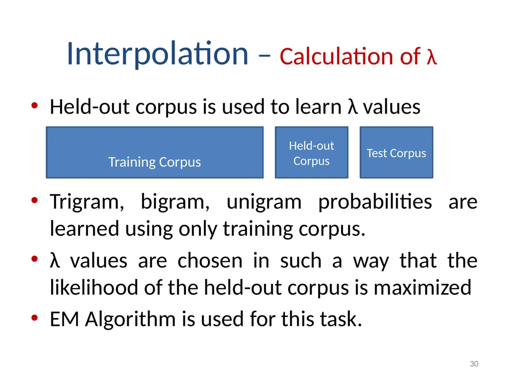
Interpolation – Calculation of λ Held-out corpus is used to learn λ values
Trigram, bigram, unigram probabilities are learned using only training corpus.
λ values are chosen in such a way that the likelihood of the held-out corpus is maximized
EM Algorithm is used for this task. 30 Training Corpus Held-out Corpus Test Corpus<br>
Trigram, bigram, unigram probabilities are learned using only training corpus.
λ values are chosen in such a way that the likelihood of the held-out corpus is maximized
EM Algorithm is used for this task. 30 Training Corpus Held-out Corpus Test Corpus<br>
31
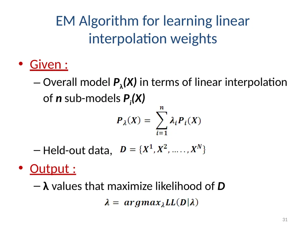
EM Algorithm for learning linear interpolation weights Given :
Overall model Pλ(X) in terms of linear interpolation of n sub-models Pi(X)
Held-out data,
Output :
λ values that maximize likelihood of D 31<br>
Overall model Pλ(X) in terms of linear interpolation of n sub-models Pi(X)
Held-out data,
Output :
λ values that maximize likelihood of D 31<br>
32
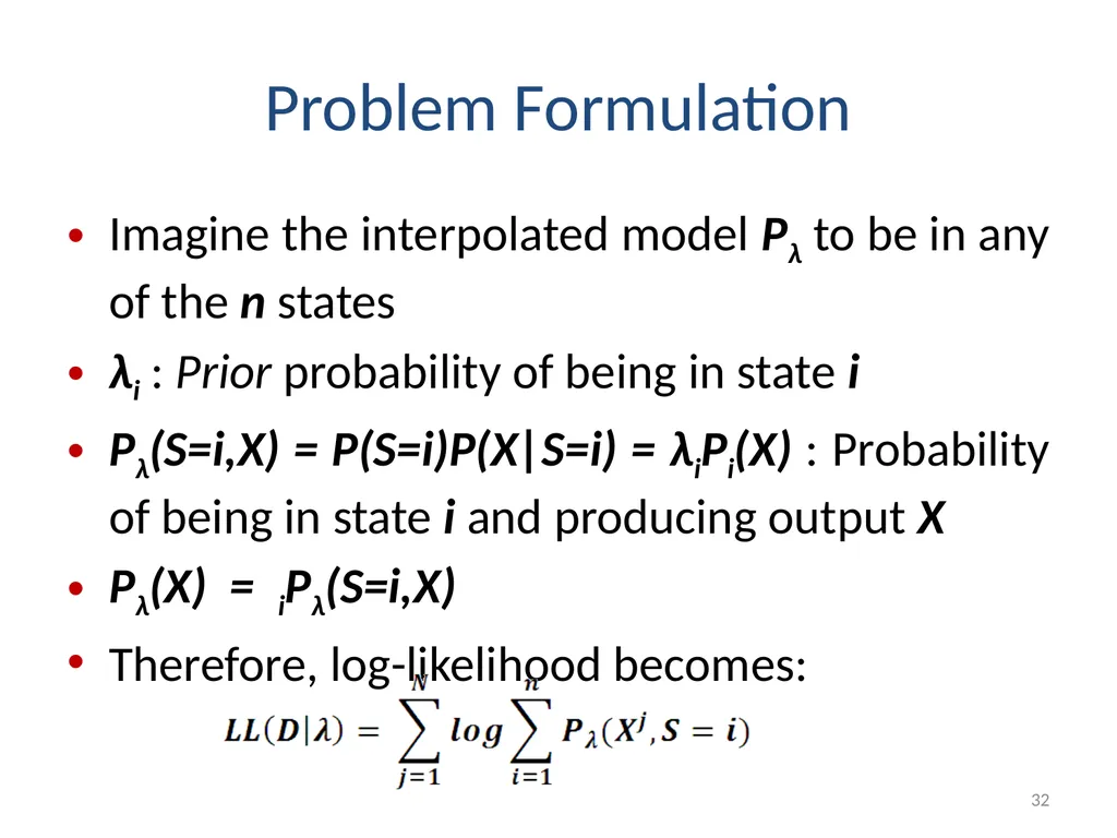
Problem Formulation Imagine the interpolated model Pλ to be in any of the n states
λi : Prior probability of being in state i
Pλ(S=i,X) = P(S=i)P(X|S=i) = λiPi(X) : Probability of being in state i and producing output X
Pλ(X) = iPλ(S=i,X)
Therefore, log-likelihood becomes: 32<br>
λi : Prior probability of being in state i
Pλ(S=i,X) = P(S=i)P(X|S=i) = λiPi(X) : Probability of being in state i and producing output X
Pλ(X) = iPλ(S=i,X)
Therefore, log-likelihood becomes: 32<br>
33
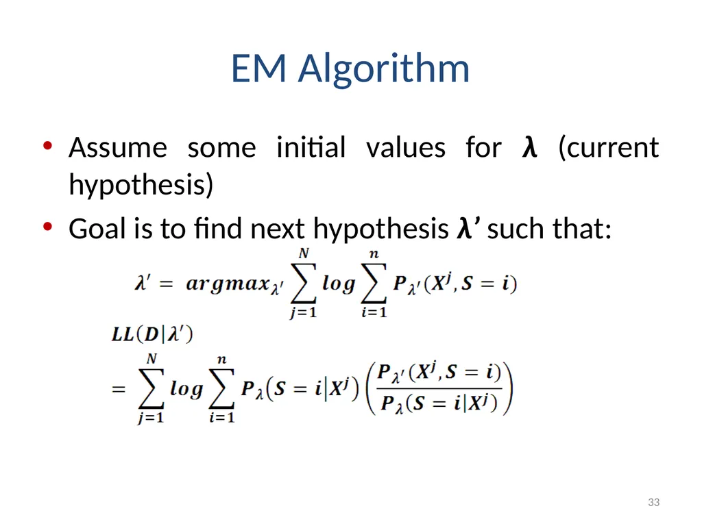
EM Algorithm Assume some initial values for λ (current hypothesis)
Goal is to find next hypothesis λ’ such that: 33<br>
Goal is to find next hypothesis λ’ such that: 33<br>
34
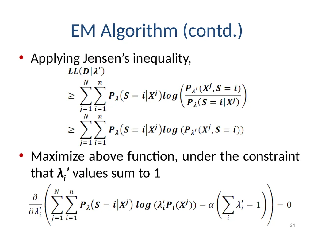
EM Algorithm (contd.) Applying Jensen’s inequality,
Maximize above function, under the constraint that λi’ values sum to 1 34<br>
Maximize above function, under the constraint that λi’ values sum to 1 34<br>
35
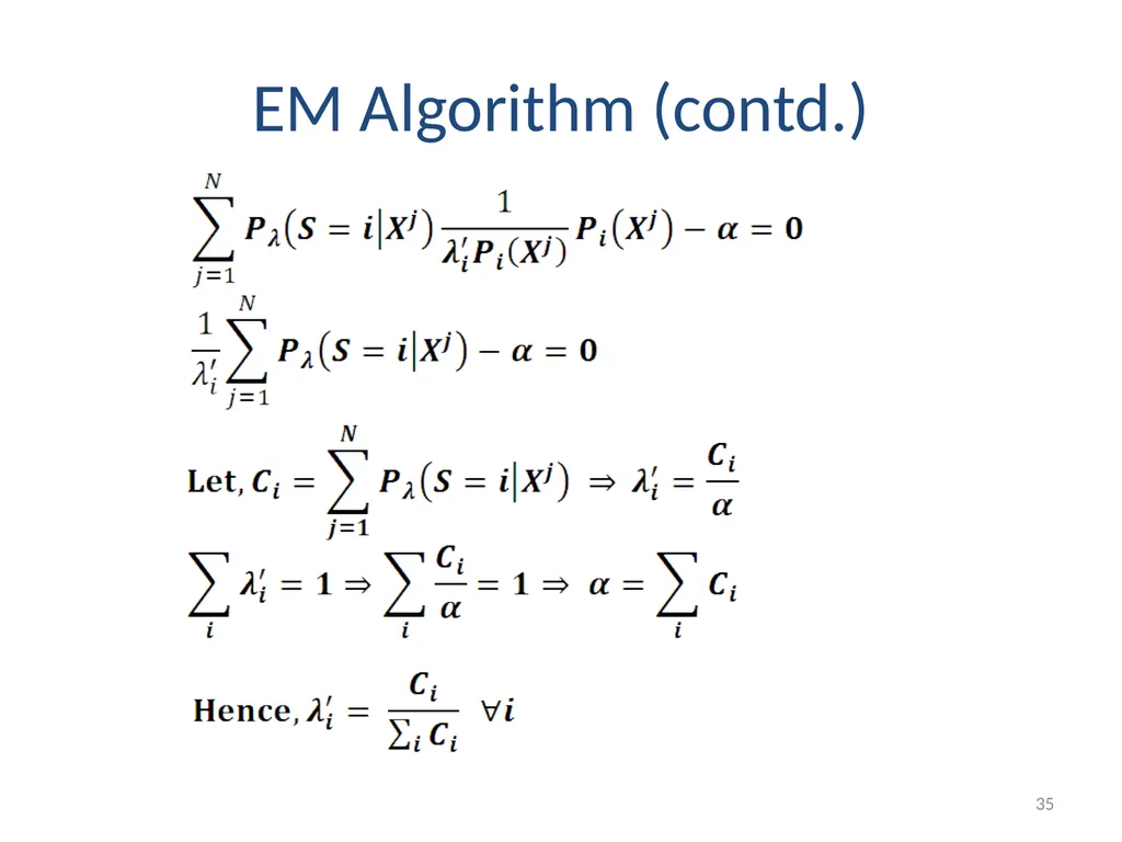
EM Algorithm (contd.) 35<br>
36
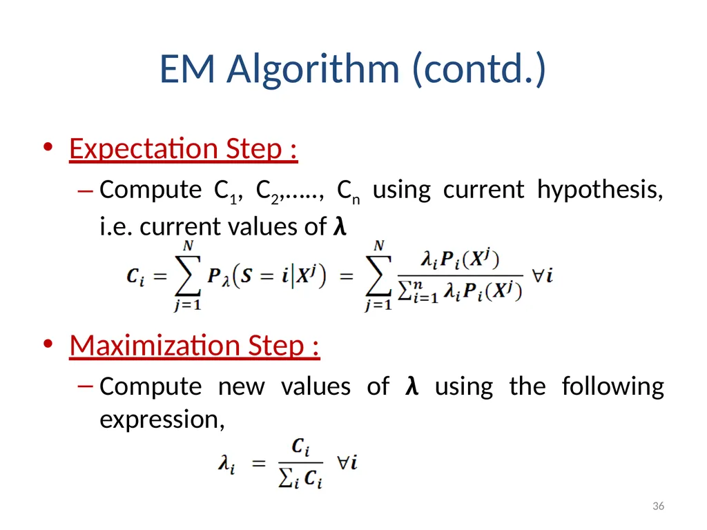
EM Algorithm (contd.) Expectation Step :
Compute C1, C2,….., Cn using current hypothesis, i.e. current values of λ
Maximization Step :
Compute new values of λ using the following expression, 36<br>
Compute C1, C2,….., Cn using current hypothesis, i.e. current values of λ
Maximization Step :
Compute new values of λ using the following expression, 36<br>
37
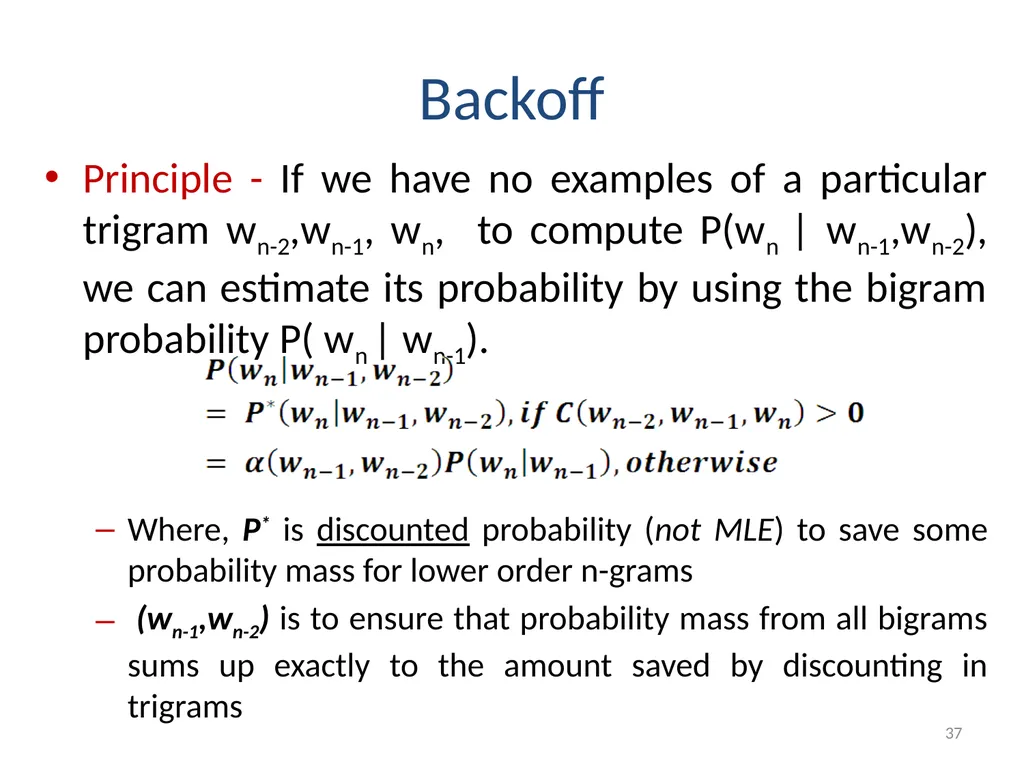
Backoff Principle - If we have no examples of a particular trigram wn-2,wn-1, wn, to compute P(wn | wn-1,wn-2), we can estimate its probability by using the bigram probability P( wn | wn-1).
Where, P* is discounted probability (not MLE) to save some probability mass for lower order n-grams
(wn-1,wn-2) is to ensure that probability mass from all bigrams sums up exactly to the amount saved by discounting in trigrams 37<br>
Where, P* is discounted probability (not MLE) to save some probability mass for lower order n-grams
(wn-1,wn-2) is to ensure that probability mass from all bigrams sums up exactly to the amount saved by discounting in trigrams 37<br>
38
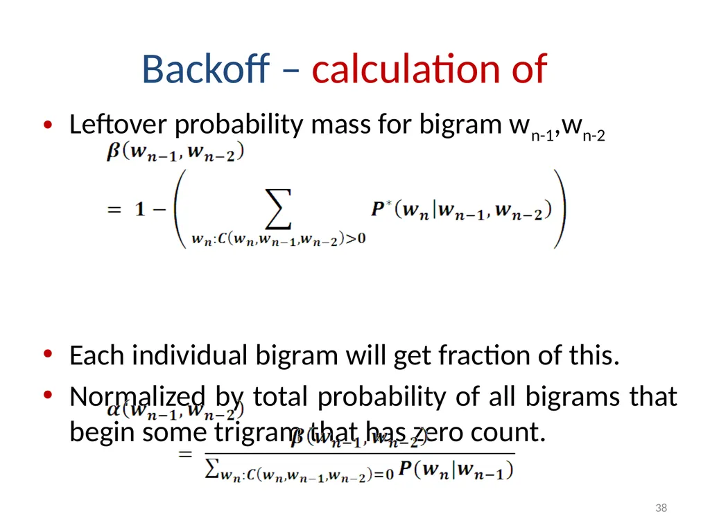
Backoff – calculation of Leftover probability mass for bigram wn-1,wn-2
Each individual bigram will get fraction of this.
Normalized by total probability of all bigrams that begin some trigram that has zero count. 38<br>
Each individual bigram will get fraction of this.
Normalized by total probability of all bigrams that begin some trigram that has zero count. 38<br>
39
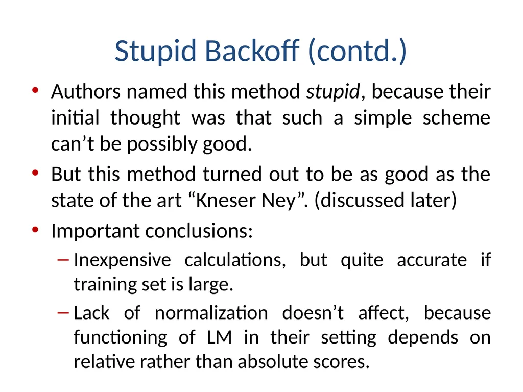
Stupid Backoff (contd.) Authors named this method stupid, because their initial thought was that such a simple scheme can’t be possibly good.
But this method turned out to be as good as the state of the art “Kneser Ney”. (discussed later)
Important conclusions:
Inexpensive calculations, but quite accurate if training set is large.
Lack of normalization doesn’t affect, because functioning of LM in their setting depends on relative rather than absolute scores.<br>
40
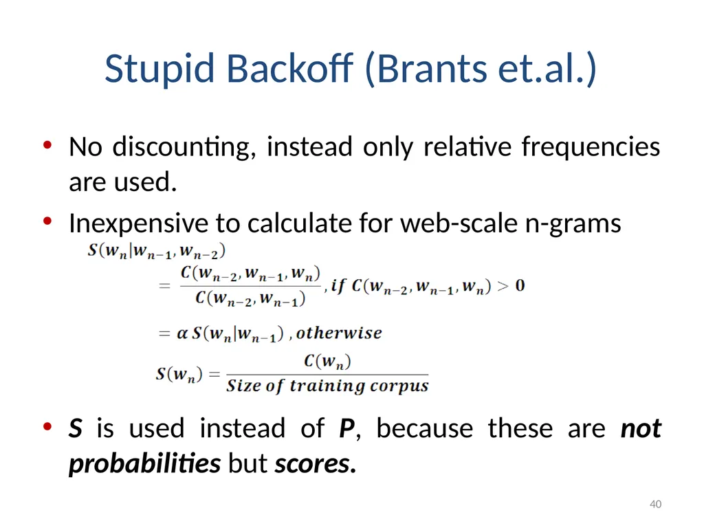
Stupid Backoff (Brants et.al.) No discounting, instead only relative frequencies are used.
Inexpensive to calculate for web-scale n-grams
S is used instead of P, because these are not probabilities but scores. 40<br>
Inexpensive to calculate for web-scale n-grams
S is used instead of P, because these are not probabilities but scores. 40<br>
41
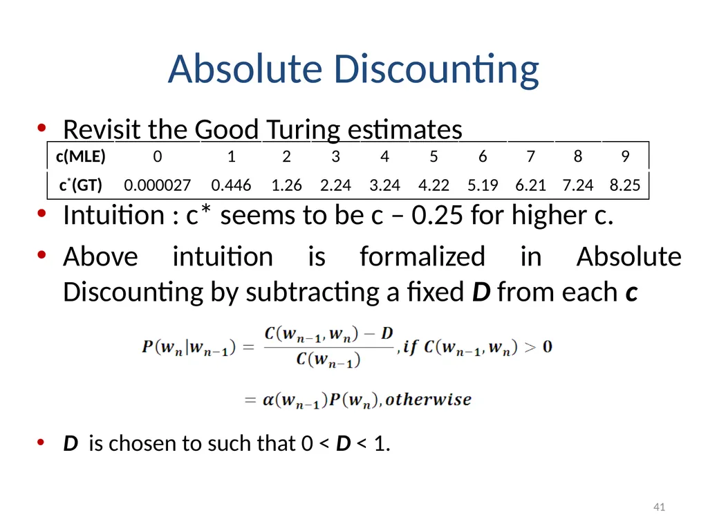
Absolute Discounting Revisit the Good Turing estimates
Intuition : c* seems to be c – 0.25 for higher c.
Above intuition is formalized in Absolute Discounting by subtracting a fixed D from each c
D is chosen to such that 0 < D < 1. 41<br>
Intuition : c* seems to be c – 0.25 for higher c.
Above intuition is formalized in Absolute Discounting by subtracting a fixed D from each c
D is chosen to such that 0 < D < 1. 41<br>
42
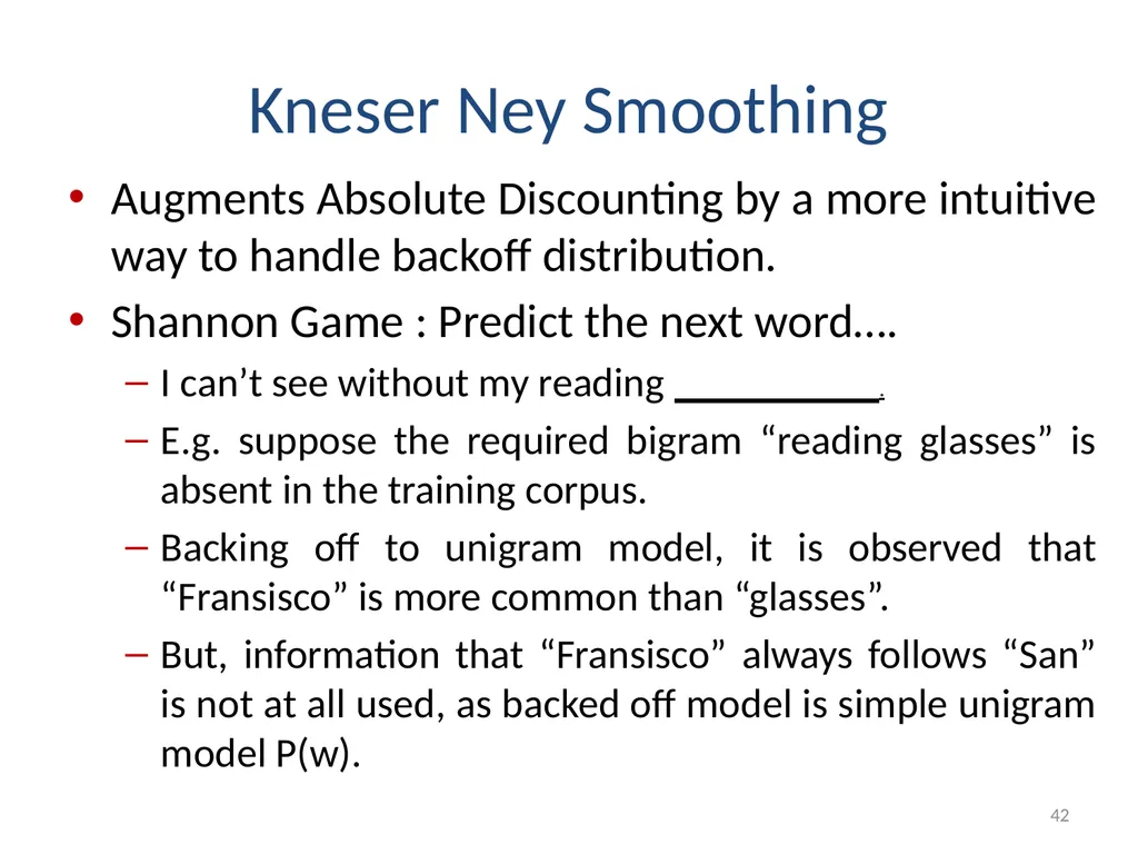
Kneser Ney Smoothing Augments Absolute Discounting by a more intuitive way to handle backoff distribution.
Shannon Game : Predict the next word….
I can’t see without my reading .
E.g. suppose the required bigram “reading glasses” is absent in the training corpus.
Backing off to unigram model, it is observed that “Fransisco” is more common than “glasses”.
But, information that “Fransisco” always follows “San” is not at all used, as backed off model is simple unigram model P(w). 42<br>
43
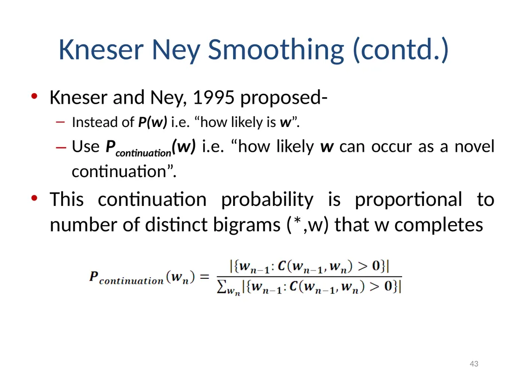
Kneser Ney Smoothing (contd.) Kneser and Ney, 1995 proposed-
Instead of P(w) i.e. “how likely is w”.
Use Pcontinuation(w) i.e. “how likely w can occur as a novel continuation”.
This continuation probability is proportional to number of distinct bigrams (*,w) that w completes 43<br>
Instead of P(w) i.e. “how likely is w”.
Use Pcontinuation(w) i.e. “how likely w can occur as a novel continuation”.
This continuation probability is proportional to number of distinct bigrams (*,w) that w completes 43<br>
44
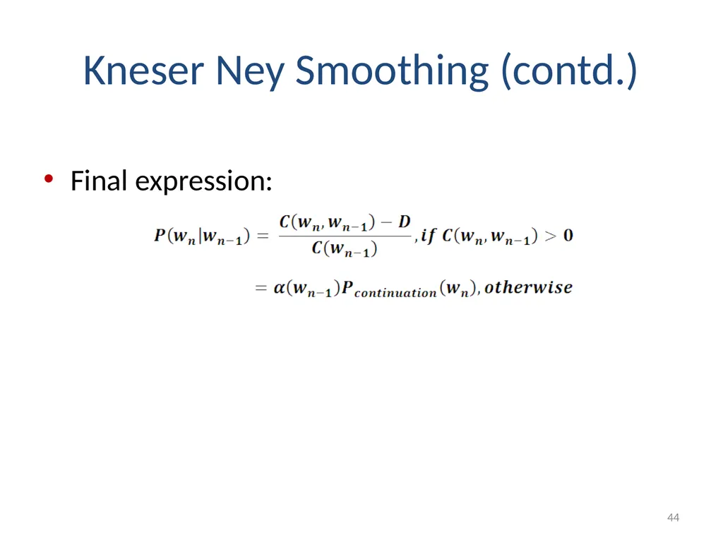
Kneser Ney Smoothing (contd.) Final expression: 44<br>
45
Short Summary Applications like Text Categorization
Add one smoothing can be used.
State of the art technique
Kneser Ney Smoothing - both interpolation and backoff versions can be used.
Very large training set like web data
like Stupid Backoff are more efficient.<br>
Add one smoothing can be used.
State of the art technique
Kneser Ney Smoothing - both interpolation and backoff versions can be used.
Very large training set like web data
like Stupid Backoff are more efficient.<br>
46
Performance of Smoothing techniques The relative performance of smoothing techniques can vary over training set size, n-gram order, and training corpus.
Back-off Vs Interpolation – For low counts, lower order distributions provide valuable information about the correct amount to discount, and thus interpolation is superior for these situations. 46<br>
Back-off Vs Interpolation – For low counts, lower order distributions provide valuable information about the correct amount to discount, and thus interpolation is superior for these situations. 46<br>
47
Comparison of Performance Algorithms that perform well on low counts perform well overall when low counts form a larger fraction of the total entropy i.e. small datasets. – why kesner ney performs best
Backoff is superior on large datasets because it is superior on high counts while interpolation is superior on low counts.
Since bigram models contain more high counts than trigram models on the same size data, backoff performs better on bigram models than on trigram models. 47<br>
Backoff is superior on large datasets because it is superior on high counts while interpolation is superior on low counts.
Since bigram models contain more high counts than trigram models on the same size data, backoff performs better on bigram models than on trigram models. 47<br>
48
Summary Need for Smoothing
Types of smoothing
Laplace Correction
Witten Bell
Good Turing
Kesner Ney
Backoff
Back off
Interpolation
Comparison 48<br>
Types of smoothing
Laplace Correction
Witten Bell
Good Turing
Kesner Ney
Backoff
Back off
Interpolation
Comparison 48<br>
49
References SF Chen, J Goodman , An empirical study of smoothing techniques for language modeling- Computer Speech & Language, 1999
Jurafsky, Daniel, and James H. Martin. 2009. Speech and Language Processing: An Introduction to Natural Language Processing, Speech Recognition, and Computational Linguistics. 2nd edition. Prentice-Hall.
H Ney, U Essen, R Kneser, On the estimation of `small' probabilities by leaving-one-out, Pattern Analysis and Machine Intelligence, 1995
T Brants, AC Popat, P Xu, FJ Och, J Dean, Large language models in machine translation, EMNLP 2007
Adam Berger, Convexity, Maximum Likelihood and All That, Tutorial at http://www.cs.cmu.edu/~aberger/maxent.html
Jurafsky’s video lecture on Language Modelling : http://www.youtube.com/watch?v=XdjCCkFUBKU 49<br>