
Soccer Video Analysis EE 368: Spring 2012 Kevin





Description: Soccer Video Analysis EE 368: Spring 2012 Kevin Cheng To detect and track key features needed to interpret events in a Soccer game from a video Goal Clip Overview Frame Pre-Processing Input Image Field Detector Field detector is trained
Related Topics
Download Presentation
"Soccer Video Analysis EE 368: Spring 2012 Kevin" is the property of its rightful owner. Permission is granted to download and print the materials on this website for personal, non-commercial use only, and to display it on your personal computer provided you do not modify the materials and that you retain all copyright notices contained in the materials. By downloading content from our website, you accept the terms of this agreement.
Presentation Transcript
slide1. Soccer Video Analysis EE 368: Spring 2012
Kevin Cheng<br>
slide2. To detect and track key features needed to interpret events in a Soccer game from a video Goal<br>
slide3. Clip<br>
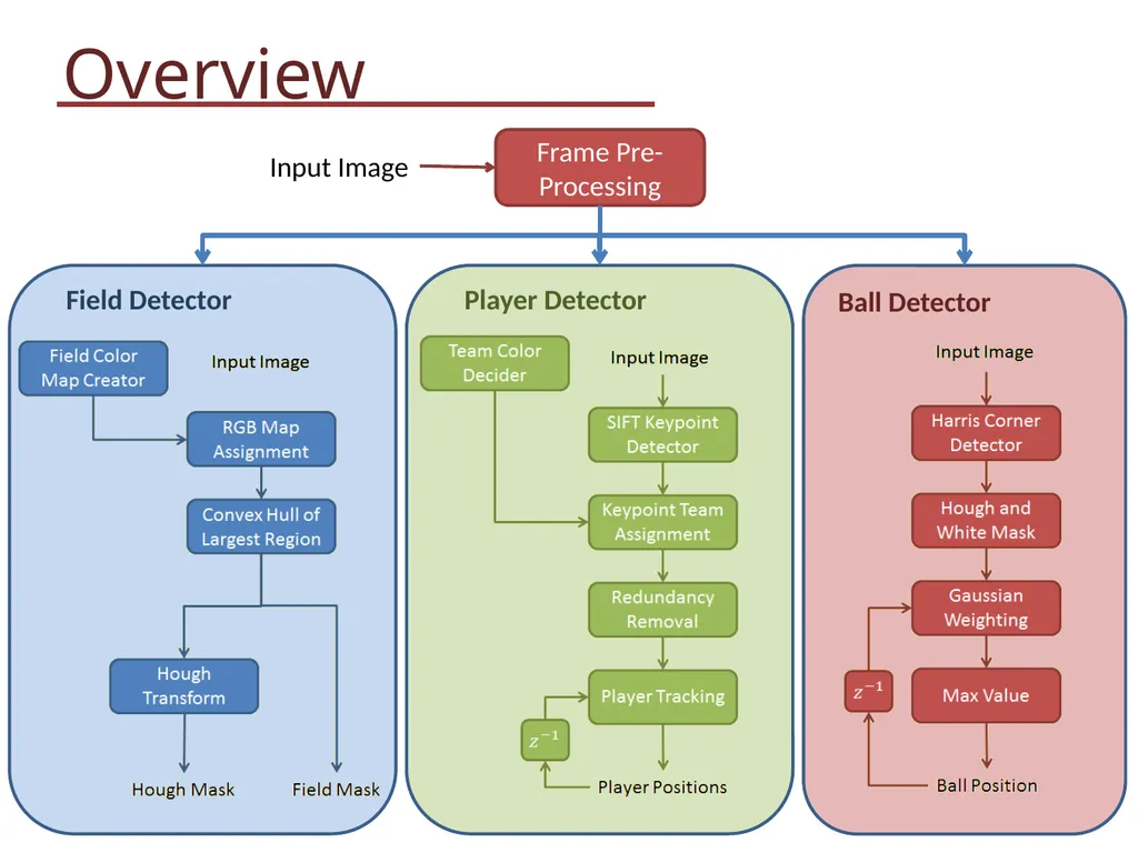
slide4. Overview Frame Pre-Processing Input Image<br>
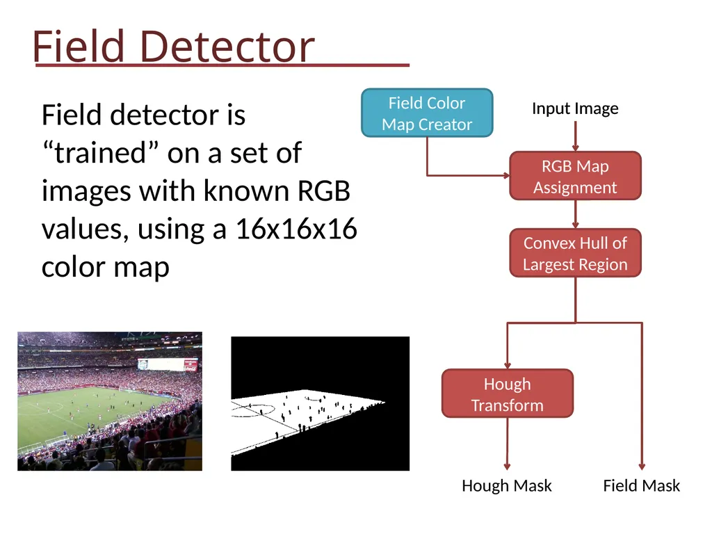
slide5. Field Detector Field detector is “trained” on a set of images with known RGB values, using a 16x16x16 color map<br>
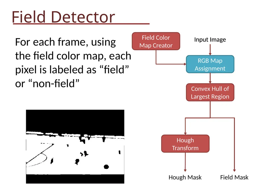
slide6. Field Detector For each frame, using the field color map, each pixel is labeled as “field” or “non-field”<br>
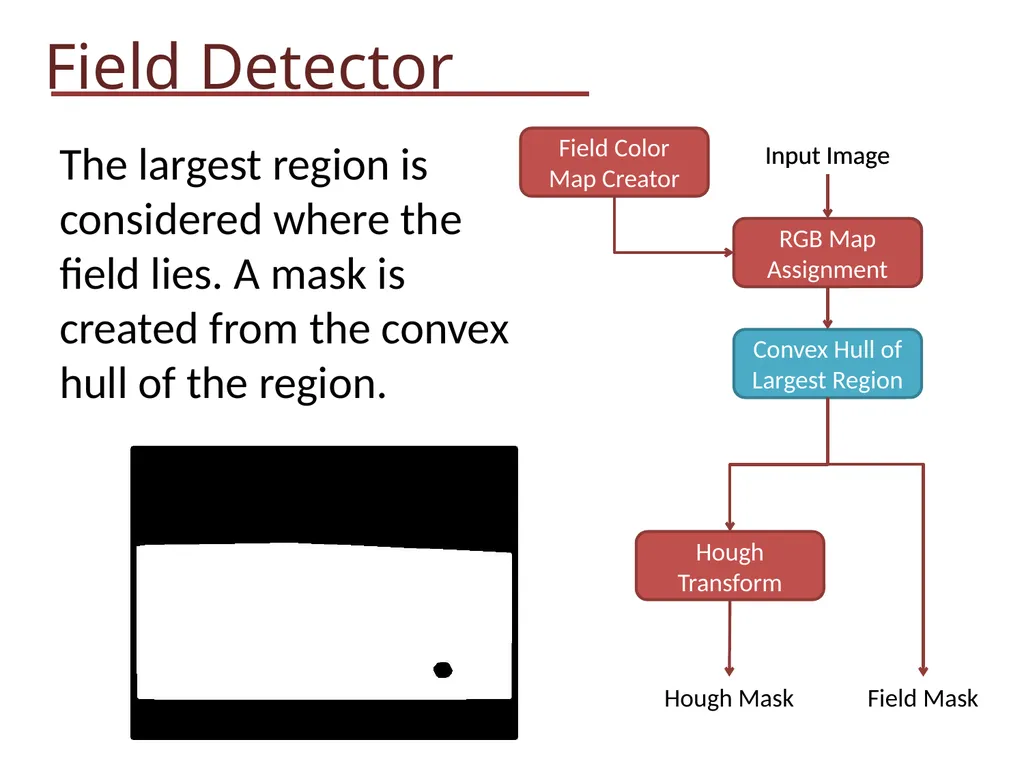
slide7. Field Detector The largest region is considered where the field lies. A mask is created from the convex hull of the region.<br>
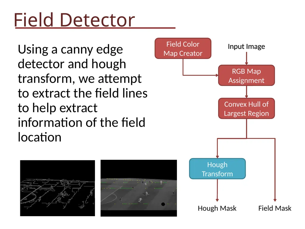
slide8. Field Detector Using a canny edge detector and hough transform, we attempt to extract the field lines to help extract information of the field location<br>
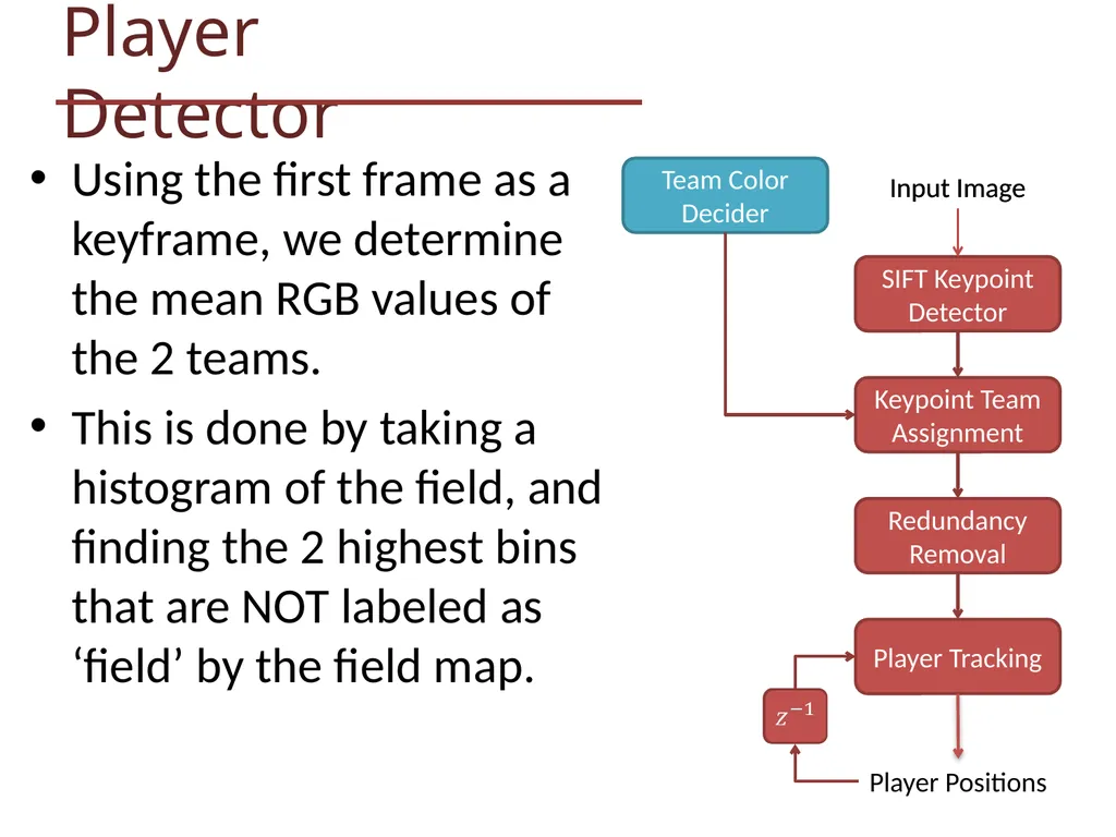
slide9. Player Detector Using the first frame as a keyframe, we determine the mean RGB values of the 2 teams.
This is done by taking a histogram of the field, and finding the 2 highest bins that are NOT labeled as ‘field’ by the field map.<br>
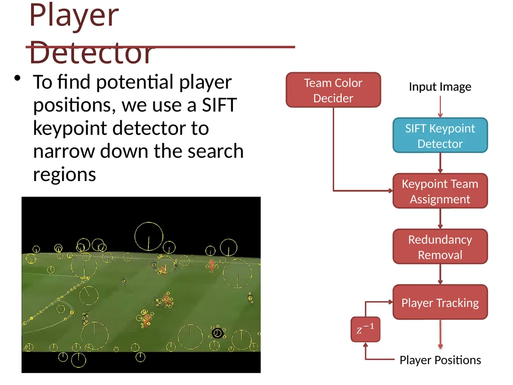
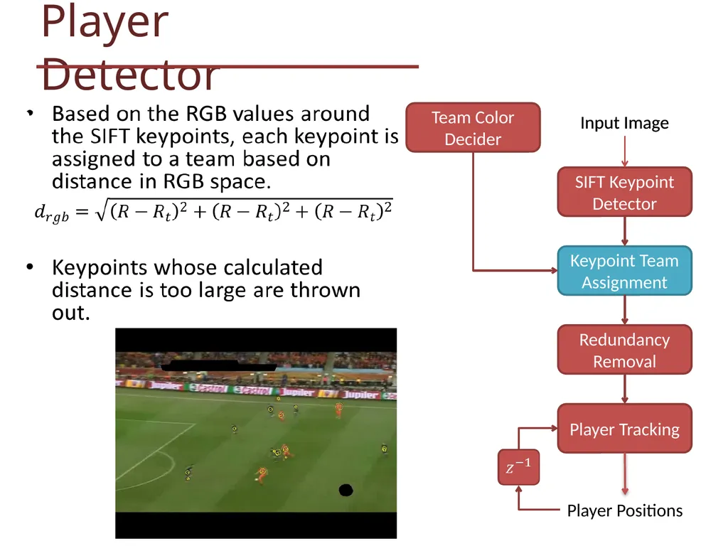
slide10. Player Detector To find potential player positions, we use a SIFT keypoint detector to narrow down the search regions<br>
slide11. Player Detector<br>
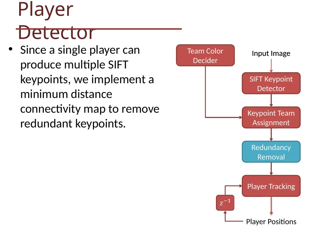
slide12. Player Detector Since a single player can produce multiple SIFT keypoints, we implement a minimum distance connectivity map to remove redundant keypoints.<br>
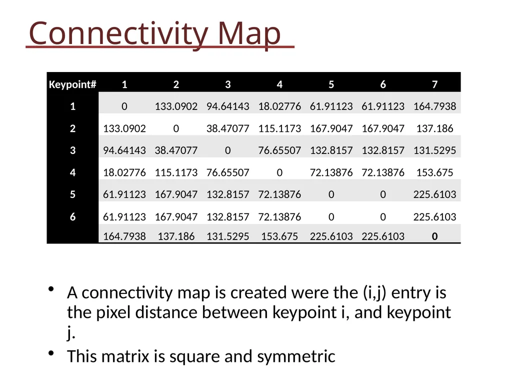
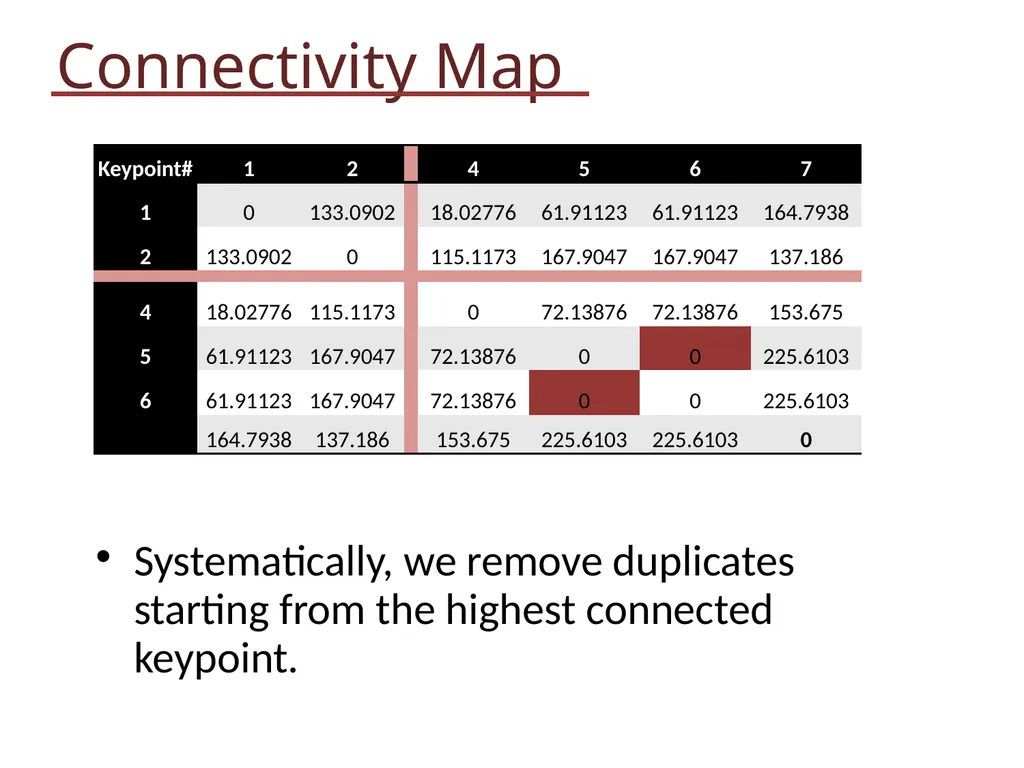
slide13. Connectivity Map A connectivity map is created were the (i,j) entry is the pixel distance between keypoint i, and keypoint j.
This matrix is square and symmetric<br>
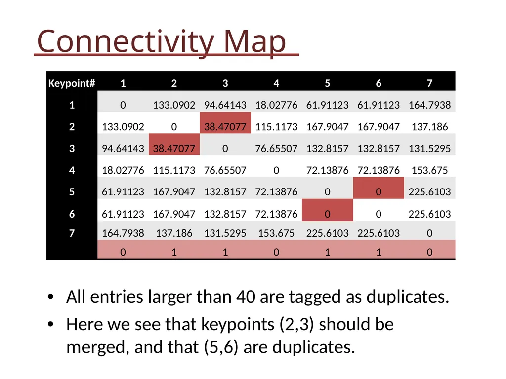
slide14. All entries larger than 40 are tagged as duplicates.
Here we see that keypoints (2,3) should be merged, and that (5,6) are duplicates. Connectivity Map<br>
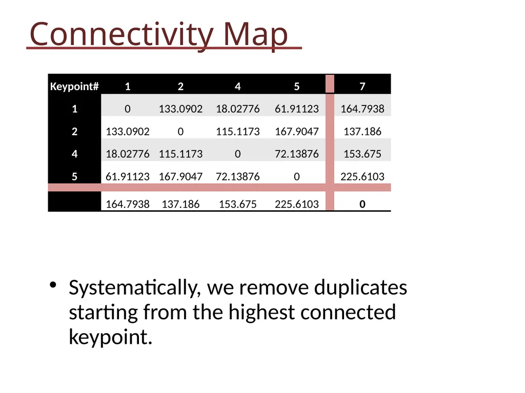
slide15. Connectivity Map Systematically, we remove duplicates starting from the highest connected keypoint.<br>
slide16. Connectivity Map Systematically, we remove duplicates starting from the highest connected keypoint.<br>
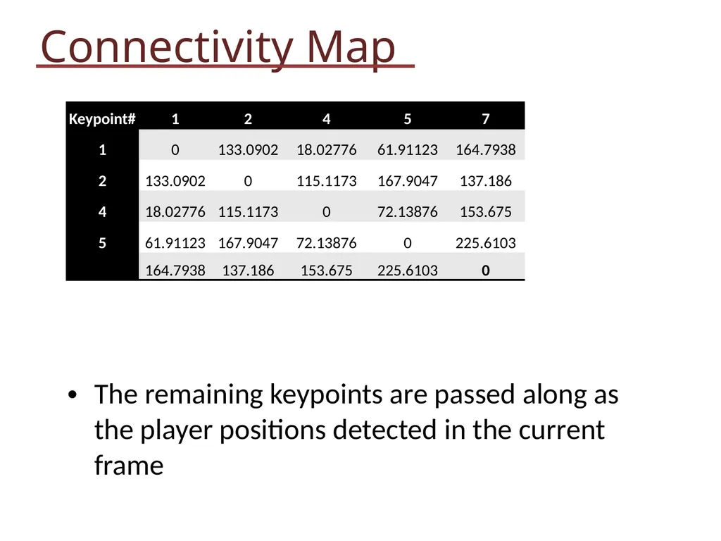
slide17. Connectivity Map The remaining keypoints are passed along as the player positions detected in the current frame<br>
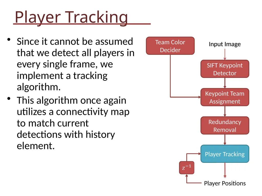
slide18. Player Tracking Since it cannot be assumed that we detect all players in every single frame, we implement a tracking algorithm.
This algorithm once again utilizes a connectivity map to match current detections with history element.<br>
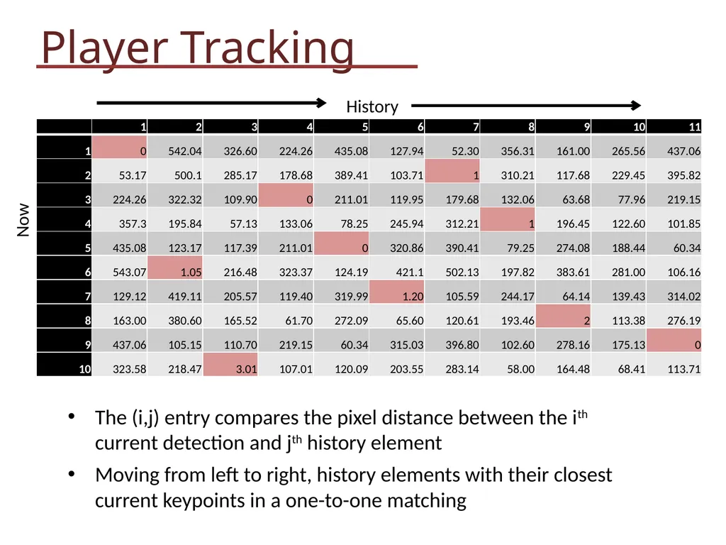
slide19. History Now Player Tracking The (i,j) entry compares the pixel distance between the ith current detection and jth history element
Moving from left to right, history elements with their closest current keypoints in a one-to-one matching<br>
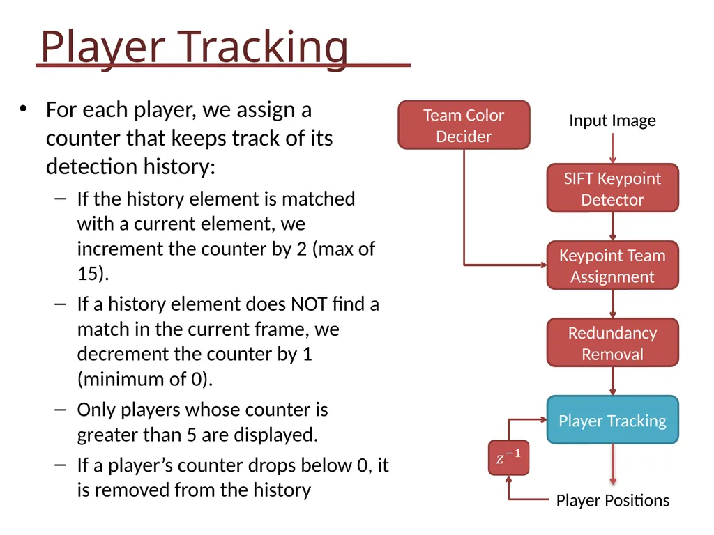
slide20. Player Tracking For each player, we assign a counter that keeps track of its detection history:
If the history element is matched with a current element, we increment the counter by 2 (max of 15).
If a history element does NOT find a match in the current frame, we decrement the counter by 1 (minimum of 0).
Only players whose counter is greater than 5 are displayed.
If a player’s counter drops below 0, it is removed from the history<br>
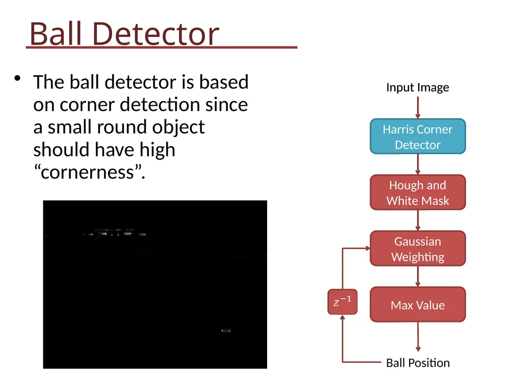
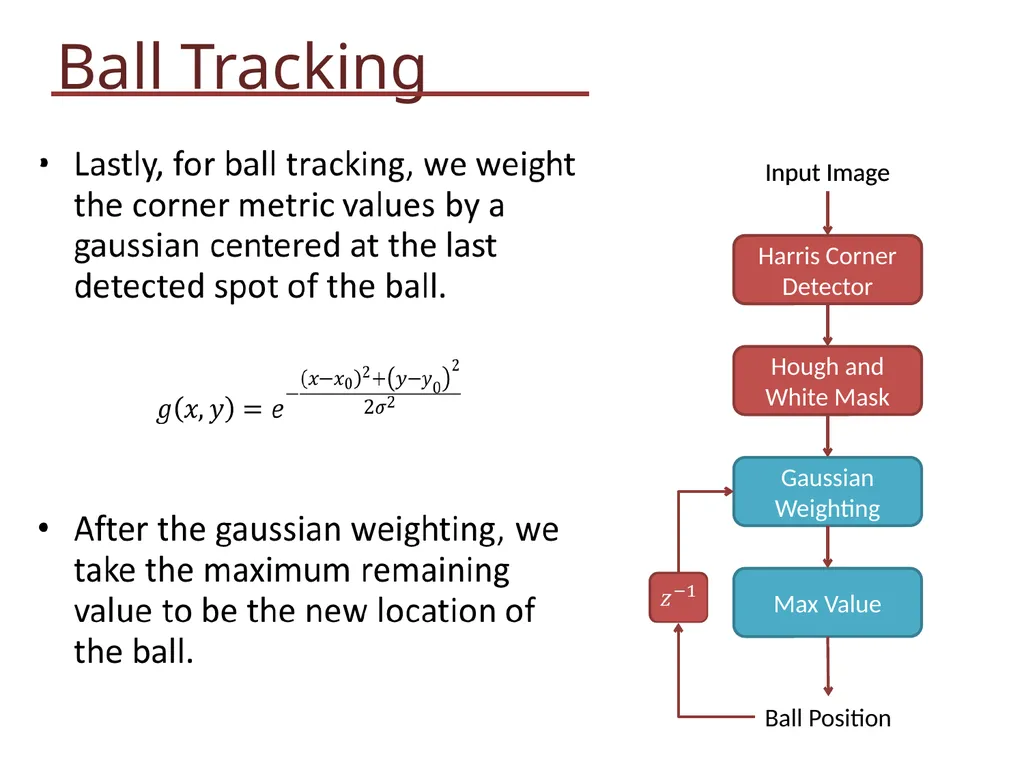
slide21. Ball Detector The ball detector is based on corner detection since a small round object should have high “cornerness”.<br>
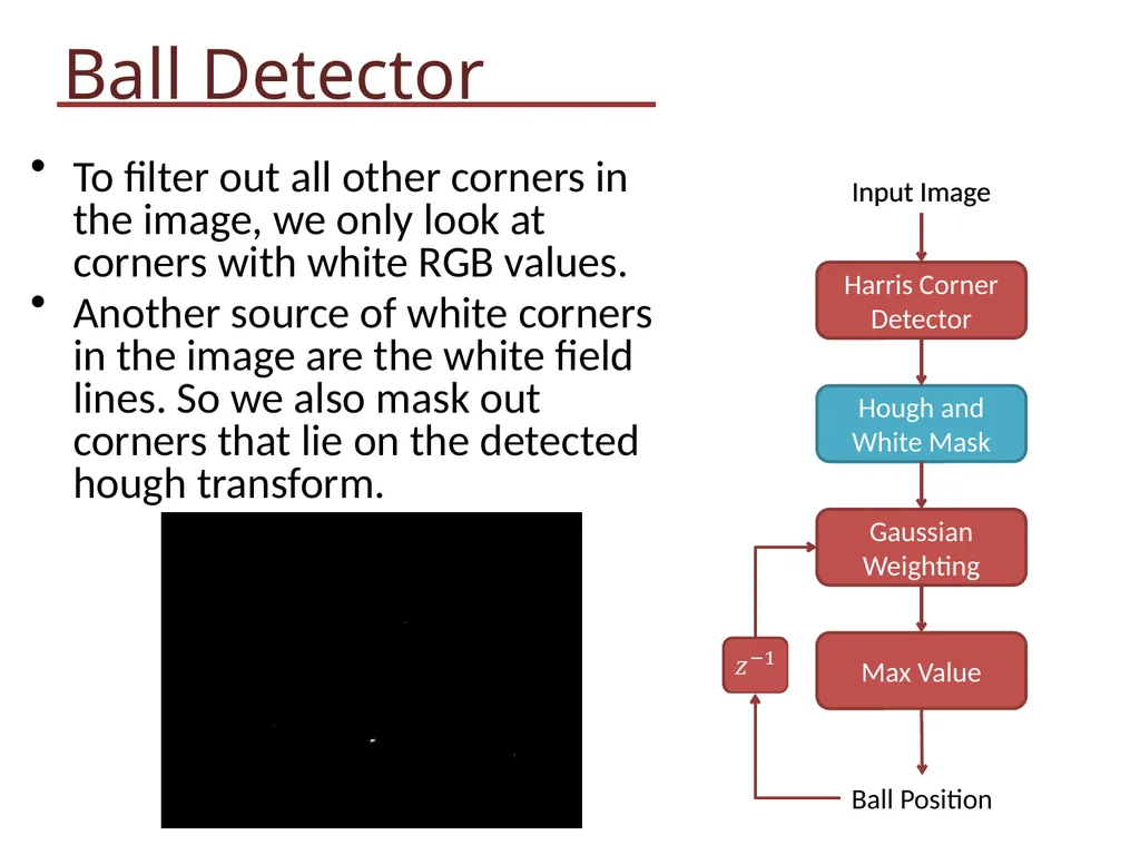
slide22. Ball Detector To filter out all other corners in the image, we only look at corners with white RGB values.
Another source of white corners in the image are the white field lines. So we also mask out corners that lie on the detected hough transform.<br>
slide23. Ball Tracking<br>
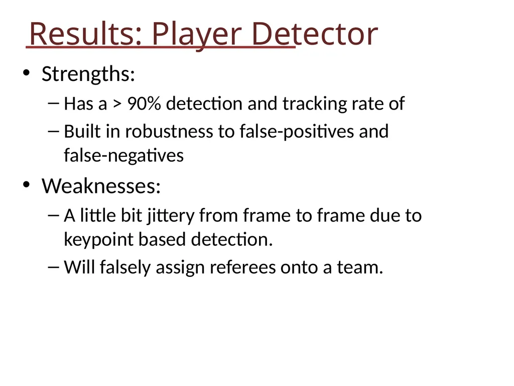
slide24. Strengths:
Has a > 90% detection and tracking rate of
Built in robustness to false-positives and false-negatives
Weaknesses:
A little bit jittery from frame to frame due to keypoint based detection.
Will falsely assign referees onto a team. Results: Player Detector<br>
slide25. Results: Player Detector<br>
slide26. Strengths:
Maintains track of ball very well
Weaknesses:
Requires to see the ball in every frame
Partial ball obscuring could cause tracker to latch onto another local maximum. Results: Ball Detector<br>
slide27. Results: Ball Detector<br>
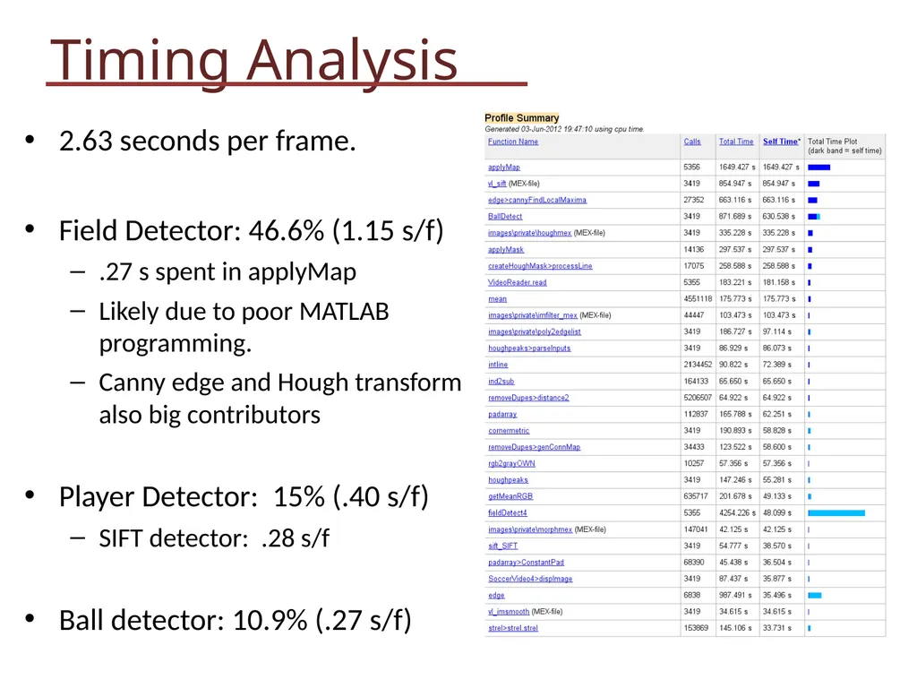
slide28. Timing Analysis 2.63 seconds per frame.
Field Detector: 46.6% (1.15 s/f)
.27 s spent in applyMap
Likely due to poor MATLAB programming.
Canny edge and Hough transform also big contributors
Player Detector: 15% (.40 s/f)
SIFT detector: .28 s/f
Ball detector: 10.9% (.27 s/f)<br>
slide29. Field Detection:
Add ability to detect where in the field you are using field lines and features.
Player Detection and Tracking:
SIFT is a large computational bottleneck. Are there more viable alternatives?
Ball Detection and Tracking:
Improve handling of cases where ball is obscured for a short amount of time.
Analysis and interpretation of detected events. Further Work<br>
Kevin Cheng<br>
slide2. To detect and track key features needed to interpret events in a Soccer game from a video Goal<br>
slide3. Clip<br>
slide4. Overview Frame Pre-Processing Input Image<br>
slide5. Field Detector Field detector is “trained” on a set of images with known RGB values, using a 16x16x16 color map<br>
slide6. Field Detector For each frame, using the field color map, each pixel is labeled as “field” or “non-field”<br>
slide7. Field Detector The largest region is considered where the field lies. A mask is created from the convex hull of the region.<br>
slide8. Field Detector Using a canny edge detector and hough transform, we attempt to extract the field lines to help extract information of the field location<br>
slide9. Player Detector Using the first frame as a keyframe, we determine the mean RGB values of the 2 teams.
This is done by taking a histogram of the field, and finding the 2 highest bins that are NOT labeled as ‘field’ by the field map.<br>
slide10. Player Detector To find potential player positions, we use a SIFT keypoint detector to narrow down the search regions<br>
slide11. Player Detector<br>
slide12. Player Detector Since a single player can produce multiple SIFT keypoints, we implement a minimum distance connectivity map to remove redundant keypoints.<br>
slide13. Connectivity Map A connectivity map is created were the (i,j) entry is the pixel distance between keypoint i, and keypoint j.
This matrix is square and symmetric<br>
slide14. All entries larger than 40 are tagged as duplicates.
Here we see that keypoints (2,3) should be merged, and that (5,6) are duplicates. Connectivity Map<br>
slide15. Connectivity Map Systematically, we remove duplicates starting from the highest connected keypoint.<br>
slide16. Connectivity Map Systematically, we remove duplicates starting from the highest connected keypoint.<br>
slide17. Connectivity Map The remaining keypoints are passed along as the player positions detected in the current frame<br>
slide18. Player Tracking Since it cannot be assumed that we detect all players in every single frame, we implement a tracking algorithm.
This algorithm once again utilizes a connectivity map to match current detections with history element.<br>
slide19. History Now Player Tracking The (i,j) entry compares the pixel distance between the ith current detection and jth history element
Moving from left to right, history elements with their closest current keypoints in a one-to-one matching<br>
slide20. Player Tracking For each player, we assign a counter that keeps track of its detection history:
If the history element is matched with a current element, we increment the counter by 2 (max of 15).
If a history element does NOT find a match in the current frame, we decrement the counter by 1 (minimum of 0).
Only players whose counter is greater than 5 are displayed.
If a player’s counter drops below 0, it is removed from the history<br>
slide21. Ball Detector The ball detector is based on corner detection since a small round object should have high “cornerness”.<br>
slide22. Ball Detector To filter out all other corners in the image, we only look at corners with white RGB values.
Another source of white corners in the image are the white field lines. So we also mask out corners that lie on the detected hough transform.<br>
slide23. Ball Tracking<br>
slide24. Strengths:
Has a > 90% detection and tracking rate of
Built in robustness to false-positives and false-negatives
Weaknesses:
A little bit jittery from frame to frame due to keypoint based detection.
Will falsely assign referees onto a team. Results: Player Detector<br>
slide25. Results: Player Detector<br>
slide26. Strengths:
Maintains track of ball very well
Weaknesses:
Requires to see the ball in every frame
Partial ball obscuring could cause tracker to latch onto another local maximum. Results: Ball Detector<br>
slide27. Results: Ball Detector<br>
slide28. Timing Analysis 2.63 seconds per frame.
Field Detector: 46.6% (1.15 s/f)
.27 s spent in applyMap
Likely due to poor MATLAB programming.
Canny edge and Hough transform also big contributors
Player Detector: 15% (.40 s/f)
SIFT detector: .28 s/f
Ball detector: 10.9% (.27 s/f)<br>
slide29. Field Detection:
Add ability to detect where in the field you are using field lines and features.
Player Detection and Tracking:
SIFT is a large computational bottleneck. Are there more viable alternatives?
Ball Detection and Tracking:
Improve handling of cases where ball is obscured for a short amount of time.
Analysis and interpretation of detected events. Further Work<br>