
Statistical Data Analysis Prof. Dr. Nizamettin
TG
Published · 62 slides · 0 views
1 / 1

Description
Statistical Data Analysis Prof. Dr. Nizamettin AYDIN naydinyildiz.edu.tr http:www3.yildiz.edu.trnaydin 1 Probability 2 Probability as a Measure of Uncertainty Plots and summary statistics are used to learn about the distribution of
Related Topics
Share
Embed code
Download this presentation From Below
"Statistical Data Analysis Prof. Dr. Nizamettin" is the property of its rightful owner. Permission is granted to download and print the materials on this website for personal, non-commercial use only, and to display it on your personal computer provided you do not modify the materials and that you retain all copyright notices contained in the materials. By downloading content from our website, you accept the terms of this agreement.
Presentation Transcript
01
Statistical Data Analysis Prof. Dr. Nizamettin AYDIN
naydin@yildiz.edu.tr
http://www3.yildiz.edu.tr/~naydin 1<br>
naydin@yildiz.edu.tr
http://www3.yildiz.edu.tr/~naydin 1<br>
02
Probability 2<br>
03
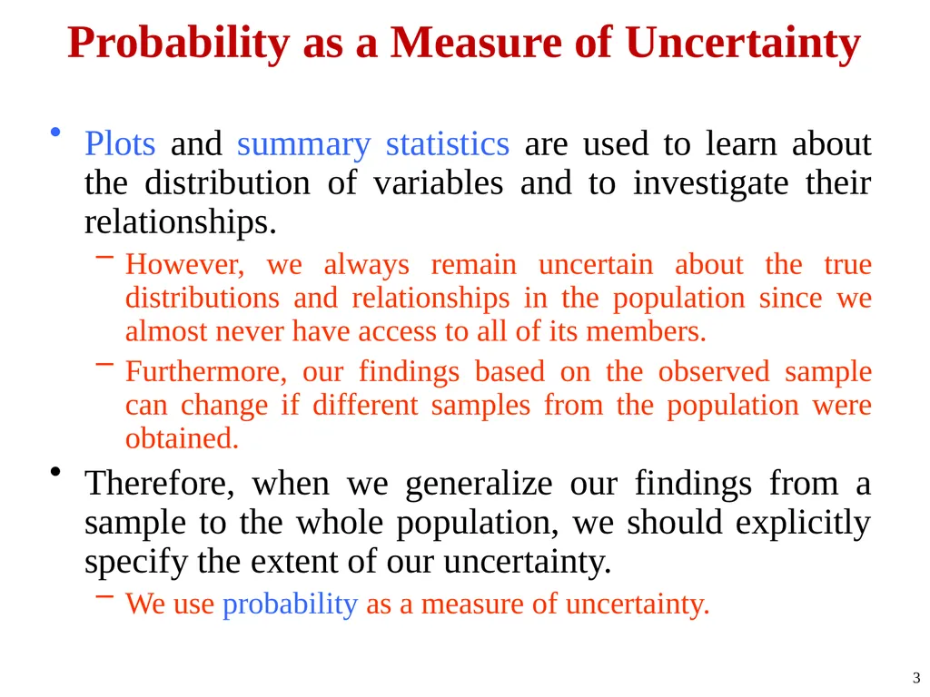
Probability as a Measure of Uncertainty Plots and summary statistics are used to learn about the distribution of variables and to investigate their relationships.
However, we always remain uncertain about the true distributions and relationships in the population since we almost never have access to all of its members.
Furthermore, our findings based on the observed sample can change if different samples from the population were obtained.
Therefore, when we generalize our findings from a sample to the whole population, we should explicitly specify the extent of our uncertainty.
We use probability as a measure of uncertainty. 3<br>
However, we always remain uncertain about the true distributions and relationships in the population since we almost never have access to all of its members.
Furthermore, our findings based on the observed sample can change if different samples from the population were obtained.
Therefore, when we generalize our findings from a sample to the whole population, we should explicitly specify the extent of our uncertainty.
We use probability as a measure of uncertainty. 3<br>
04
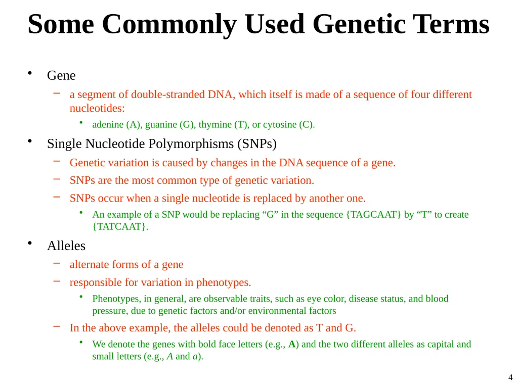
Some Commonly Used Genetic Terms Gene
a segment of double-stranded DNA, which itself is made of a sequence of four different nucleotides:
adenine (A), guanine (G), thymine (T), or cytosine (C).
Single Nucleotide Polymorphisms (SNPs)
Genetic variation is caused by changes in the DNA sequence of a gene.
SNPs are the most common type of genetic variation.
SNPs occur when a single nucleotide is replaced by another one.
An example of a SNP would be replacing “G” in the sequence {TAGCAAT} by “T” to create {TATCAAT}.
Alleles
alternate forms of a gene
responsible for variation in phenotypes.
Phenotypes, in general, are observable traits, such as eye color, disease status, and blood pressure, due to genetic factors and/or environmental factors
In the above example, the alleles could be denoted as T and G.
We denote the genes with bold face letters (e.g., A) and the two different alleles as capital and small letters (e.g., A and a). 4<br>
a segment of double-stranded DNA, which itself is made of a sequence of four different nucleotides:
adenine (A), guanine (G), thymine (T), or cytosine (C).
Single Nucleotide Polymorphisms (SNPs)
Genetic variation is caused by changes in the DNA sequence of a gene.
SNPs are the most common type of genetic variation.
SNPs occur when a single nucleotide is replaced by another one.
An example of a SNP would be replacing “G” in the sequence {TAGCAAT} by “T” to create {TATCAAT}.
Alleles
alternate forms of a gene
responsible for variation in phenotypes.
Phenotypes, in general, are observable traits, such as eye color, disease status, and blood pressure, due to genetic factors and/or environmental factors
In the above example, the alleles could be denoted as T and G.
We denote the genes with bold face letters (e.g., A) and the two different alleles as capital and small letters (e.g., A and a). 4<br>
05
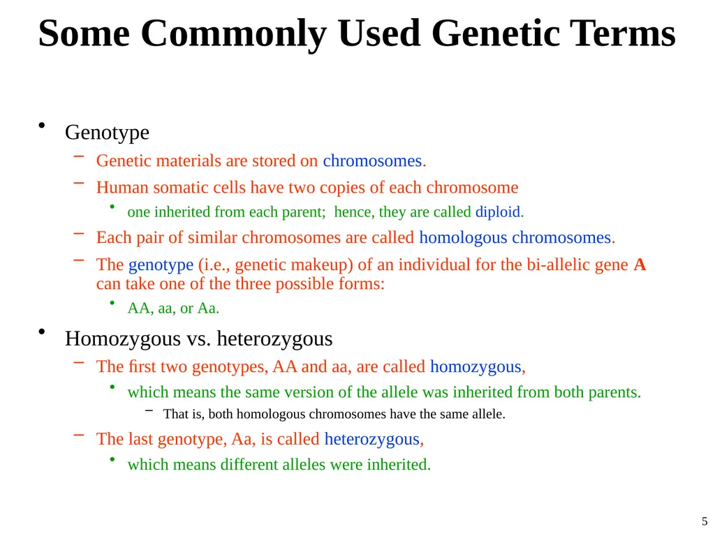
Some Commonly Used Genetic Terms Genotype
Genetic materials are stored on chromosomes.
Human somatic cells have two copies of each chromosome
one inherited from each parent; hence, they are called diploid.
Each pair of similar chromosomes are called homologous chromosomes.
The genotype (i.e., genetic makeup) of an individual for the bi-allelic gene A can take one of the three possible forms:
AA, aa, or Aa.
Homozygous vs. heterozygous
The first two genotypes, AA and aa, are called homozygous,
which means the same version of the allele was inherited from both parents.
That is, both homologous chromosomes have the same allele.
The last genotype, Aa, is called heterozygous,
which means different alleles were inherited. 5<br>
Genetic materials are stored on chromosomes.
Human somatic cells have two copies of each chromosome
one inherited from each parent; hence, they are called diploid.
Each pair of similar chromosomes are called homologous chromosomes.
The genotype (i.e., genetic makeup) of an individual for the bi-allelic gene A can take one of the three possible forms:
AA, aa, or Aa.
Homozygous vs. heterozygous
The first two genotypes, AA and aa, are called homozygous,
which means the same version of the allele was inherited from both parents.
That is, both homologous chromosomes have the same allele.
The last genotype, Aa, is called heterozygous,
which means different alleles were inherited. 5<br>
06
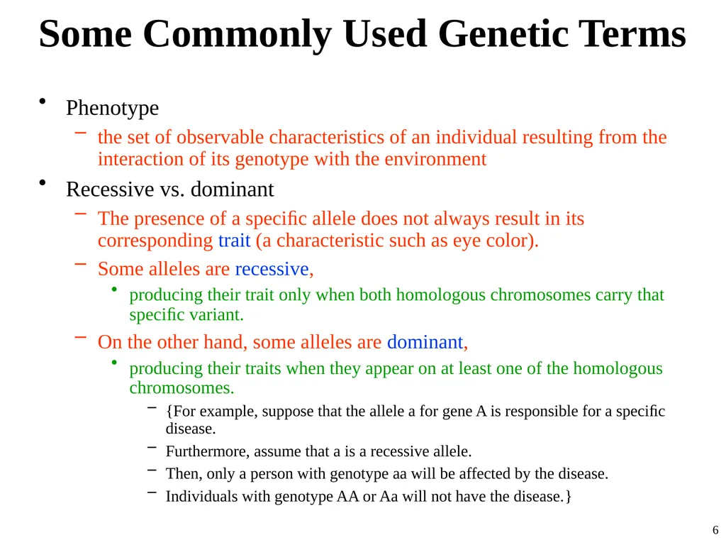
Some Commonly Used Genetic Terms Phenotype
the set of observable characteristics of an individual resulting from the interaction of its genotype with the environment
Recessive vs. dominant
The presence of a specific allele does not always result in its corresponding trait (a characteristic such as eye color).
Some alleles are recessive,
producing their trait only when both homologous chromosomes carry that specific variant.
On the other hand, some alleles are dominant,
producing their traits when they appear on at least one of the homologous chromosomes.
{For example, suppose that the allele a for gene A is responsible for a specific disease.
Furthermore, assume that a is a recessive allele.
Then, only a person with genotype aa will be affected by the disease.
Individuals with genotype AA or Aa will not have the disease.} 6<br>
the set of observable characteristics of an individual resulting from the interaction of its genotype with the environment
Recessive vs. dominant
The presence of a specific allele does not always result in its corresponding trait (a characteristic such as eye color).
Some alleles are recessive,
producing their trait only when both homologous chromosomes carry that specific variant.
On the other hand, some alleles are dominant,
producing their traits when they appear on at least one of the homologous chromosomes.
{For example, suppose that the allele a for gene A is responsible for a specific disease.
Furthermore, assume that a is a recessive allele.
Then, only a person with genotype aa will be affected by the disease.
Individuals with genotype AA or Aa will not have the disease.} 6<br>
07
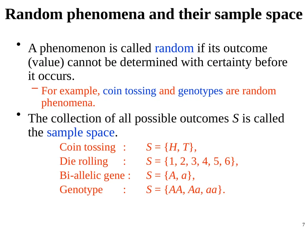
Random phenomena and their sample space A phenomenon is called random if its outcome (value) cannot be determined with certainty before it occurs.
For example, coin tossing and genotypes are random phenomena.
The collection of all possible outcomes S is called the sample space.
Coin tossing : S = {H, T},
Die rolling : S = {1, 2, 3, 4, 5, 6},
Bi-allelic gene : S = {A, a},
Genotype : S = {AA, Aa, aa}. 7<br>
For example, coin tossing and genotypes are random phenomena.
The collection of all possible outcomes S is called the sample space.
Coin tossing : S = {H, T},
Die rolling : S = {1, 2, 3, 4, 5, 6},
Bi-allelic gene : S = {A, a},
Genotype : S = {AA, Aa, aa}. 7<br>
08
Random phenomena and their sample space The sample space might include an infinite number of possible outcomes.
For example, the value of blood pressure is random since it cannot be determined with certainty before measuring it.
The corresponding sample space for blood pressure values is (theoretically) the set of positive real numbers, which is infinite.
For a complex random phenomenon that is a combination of two or more other random phenomena, it might be easier to view the sample space with tree diagrams. 8<br>
For example, the value of blood pressure is random since it cannot be determined with certainty before measuring it.
The corresponding sample space for blood pressure values is (theoretically) the set of positive real numbers, which is infinite.
For a complex random phenomenon that is a combination of two or more other random phenomena, it might be easier to view the sample space with tree diagrams. 8<br>
09
Random phenomena and their sample space For example, suppose that we suspect that gene A is related to a specific disease, but genetic variation alone does not determine the disease status.
Rather, it affects the risk of the disease.
Further, we suspect that smoking (an environmental factor) is also related to the disease.
In this case, the random phenomenon we are interested in is the combination of genotype and smoking status
All possible combinations (i.e., sample space) are identified using the following tree diagram. 9<br>
Rather, it affects the risk of the disease.
Further, we suspect that smoking (an environmental factor) is also related to the disease.
In this case, the random phenomenon we are interested in is the combination of genotype and smoking status
All possible combinations (i.e., sample space) are identified using the following tree diagram. 9<br>
10
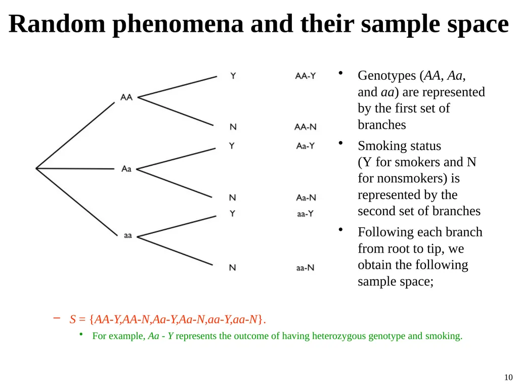
Random phenomena and their sample space Genotypes (AA, Aa, and aa) are represented by the first set of branches
Smoking status (Y for smokers and N for nonsmokers) is represented by the second set of branches
Following each branch from root to tip, we obtain the following sample space;
S = {AA-Y,AA-N,Aa-Y,Aa-N,aa-Y,aa-N}.
For example, Aa - Y represents the outcome of having heterozygous genotype and smoking. 10<br>
Smoking status (Y for smokers and N for nonsmokers) is represented by the second set of branches
Following each branch from root to tip, we obtain the following sample space;
S = {AA-Y,AA-N,Aa-Y,Aa-N,aa-Y,aa-N}.
For example, Aa - Y represents the outcome of having heterozygous genotype and smoking. 10<br>
11
Probability Measure To each possible outcome in the sample space, we assign a probability P,
which represents how certain we are about the occurrence of the corresponding outcome.
For an outcome o, we denote the probability as P(o),
where 0 ≤ P(o) ≤ 1.
The total probability of all outcomes in the sample space is always 1.
Coin tossing : P(H) + P(T) = 1
Die rolling : P(1) + P(2) + P(3) + P(4) + P(5) + P(6) = 1
Therefore, if the outcomes are equally probable,
the probability of each outcome is 1/nS,
where nS is the number of possible outcomes. 11<br>
which represents how certain we are about the occurrence of the corresponding outcome.
For an outcome o, we denote the probability as P(o),
where 0 ≤ P(o) ≤ 1.
The total probability of all outcomes in the sample space is always 1.
Coin tossing : P(H) + P(T) = 1
Die rolling : P(1) + P(2) + P(3) + P(4) + P(5) + P(6) = 1
Therefore, if the outcomes are equally probable,
the probability of each outcome is 1/nS,
where nS is the number of possible outcomes. 11<br>
12
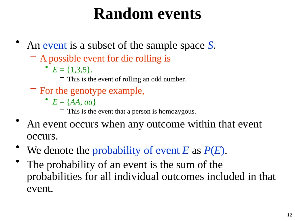
Random events An event is a subset of the sample space S.
A possible event for die rolling is
E = {1,3,5}.
This is the event of rolling an odd number.
For the genotype example,
E = {AA, aa}
This is the event that a person is homozygous.
An event occurs when any outcome within that event occurs.
We denote the probability of event E as P(E).
The probability of an event is the sum of the probabilities for all individual outcomes included in that event. 12<br>
A possible event for die rolling is
E = {1,3,5}.
This is the event of rolling an odd number.
For the genotype example,
E = {AA, aa}
This is the event that a person is homozygous.
An event occurs when any outcome within that event occurs.
We denote the probability of event E as P(E).
The probability of an event is the sum of the probabilities for all individual outcomes included in that event. 12<br>
13
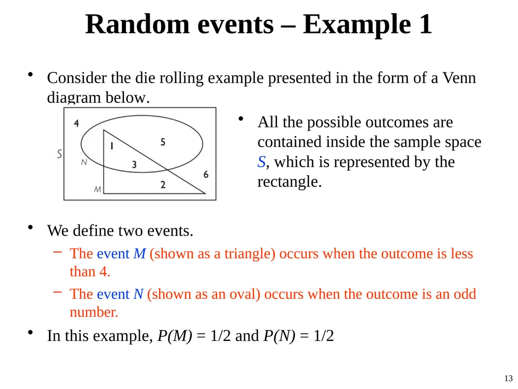
Random events – Example 1 Consider the die rolling example presented in the form of a Venn diagram below.
All the possible outcomes are contained inside the sample space S, which is represented by the rectangle.
We define two events.
The event M (shown as a triangle) occurs when the outcome is less than 4.
The event N (shown as an oval) occurs when the outcome is an odd number.
In this example, P(M) = 1/2 and P(N) = 1/2 13<br>
All the possible outcomes are contained inside the sample space S, which is represented by the rectangle.
We define two events.
The event M (shown as a triangle) occurs when the outcome is less than 4.
The event N (shown as an oval) occurs when the outcome is an odd number.
In this example, P(M) = 1/2 and P(N) = 1/2 13<br>
14
Random events – Example 2 As a running example, we consider a bi-allelic gene A with two alleles A and a.
We assume that allele a is recessive and causes a specific disease.
Then only people with the genotype aa have the disease.
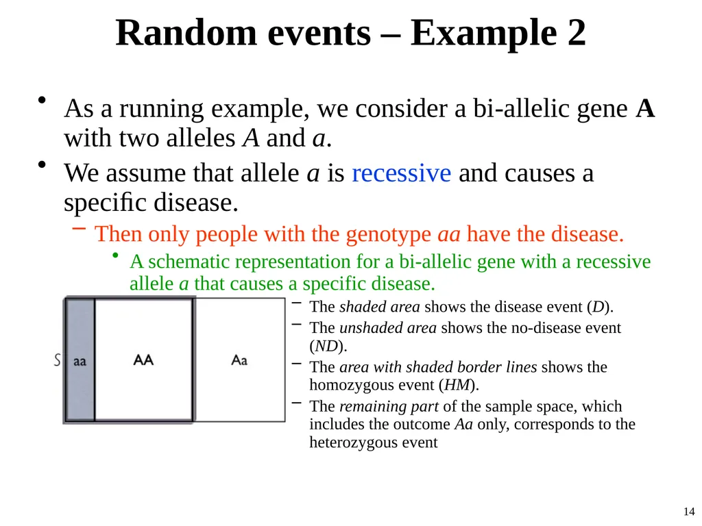
A schematic representation for a bi-allelic gene with a recessive allele a that causes a specific disease.
The shaded area shows the disease event (D).
The unshaded area shows the no-disease event (ND).
The area with shaded border lines shows the homozygous event (HM).
The remaining part of the sample space, which includes the outcome Aa only, corresponds to the heterozygous event 14<br>
We assume that allele a is recessive and causes a specific disease.
Then only people with the genotype aa have the disease.
A schematic representation for a bi-allelic gene with a recessive allele a that causes a specific disease.
The shaded area shows the disease event (D).
The unshaded area shows the no-disease event (ND).
The area with shaded border lines shows the homozygous event (HM).
The remaining part of the sample space, which includes the outcome Aa only, corresponds to the heterozygous event 14<br>
15
Random events - Example We can define four events as follows:
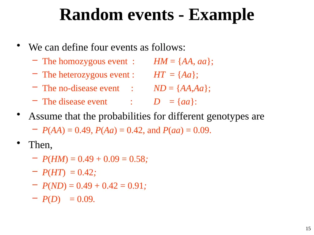
The homozygous event : HM = {AA, aa};
The heterozygous event : HT = {Aa};
The no-disease event : ND = {AA,Aa};
The disease event : D = {aa}:
Assume that the probabilities for different genotypes are
P(AA) = 0.49, P(Aa) = 0.42, and P(aa) = 0.09.
Then,
P(HM) = 0.49 + 0.09 = 0.58;
P(HT) = 0.42;
P(ND) = 0.49 + 0.42 = 0.91;
P(D) = 0.09. 15<br>
The homozygous event : HM = {AA, aa};
The heterozygous event : HT = {Aa};
The no-disease event : ND = {AA,Aa};
The disease event : D = {aa}:
Assume that the probabilities for different genotypes are
P(AA) = 0.49, P(Aa) = 0.42, and P(aa) = 0.09.
Then,
P(HM) = 0.49 + 0.09 = 0.58;
P(HT) = 0.42;
P(ND) = 0.49 + 0.42 = 0.91;
P(D) = 0.09. 15<br>
16
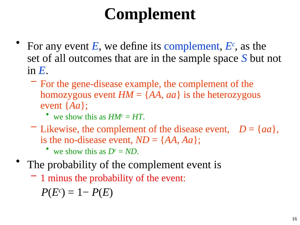
Complement For any event E, we define its complement, Ec, as the set of all outcomes that are in the sample space S but not in E.
For the gene-disease example, the complement of the homozygous event HM = {AA, aa} is the heterozygous event {Aa};
we show this as HMc = HT.
Likewise, the complement of the disease event, D = {aa}, is the no-disease event, ND = {AA, Aa};
we show this as Dc = ND.
The probability of the complement event is
1 minus the probability of the event:
P(Ec) = 1− P(E) 16<br>
For the gene-disease example, the complement of the homozygous event HM = {AA, aa} is the heterozygous event {Aa};
we show this as HMc = HT.
Likewise, the complement of the disease event, D = {aa}, is the no-disease event, ND = {AA, Aa};
we show this as Dc = ND.
The probability of the complement event is
1 minus the probability of the event:
P(Ec) = 1− P(E) 16<br>
17
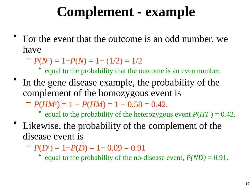
Complement - example For the event that the outcome is an odd number, we have
P(Nc) = 1−P(N) = 1− (1/2) = 1/2
equal to the probability that the outcome is an even number.
In the gene disease example, the probability of the complement of the homozygous event is
P(HMc) = 1 − P(HM) = 1 − 0.58 = 0.42.
equal to the probability of the heterozygous event P(HT ) = 0.42.
Likewise, the probability of the complement of the disease event is
P(Dc) = 1−P(D) = 1− 0.09 = 0.91
equal to the probability of the no-disease event, P(ND) = 0.91. 17<br>
P(Nc) = 1−P(N) = 1− (1/2) = 1/2
equal to the probability that the outcome is an even number.
In the gene disease example, the probability of the complement of the homozygous event is
P(HMc) = 1 − P(HM) = 1 − 0.58 = 0.42.
equal to the probability of the heterozygous event P(HT ) = 0.42.
Likewise, the probability of the complement of the disease event is
P(Dc) = 1−P(D) = 1− 0.09 = 0.91
equal to the probability of the no-disease event, P(ND) = 0.91. 17<br>
18
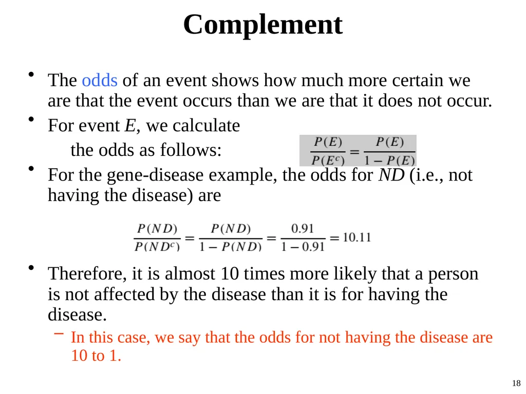
Complement The odds of an event shows how much more certain we are that the event occurs than we are that it does not occur.
For event E, we calculate
the odds as follows:
For the gene-disease example, the odds for ND (i.e., not having the disease) are
Therefore, it is almost 10 times more likely that a person is not affected by the disease than it is for having the disease.
In this case, we say that the odds for not having the disease are 10 to 1. 18<br>
For event E, we calculate
the odds as follows:
For the gene-disease example, the odds for ND (i.e., not having the disease) are
Therefore, it is almost 10 times more likely that a person is not affected by the disease than it is for having the disease.
In this case, we say that the odds for not having the disease are 10 to 1. 18<br>
19
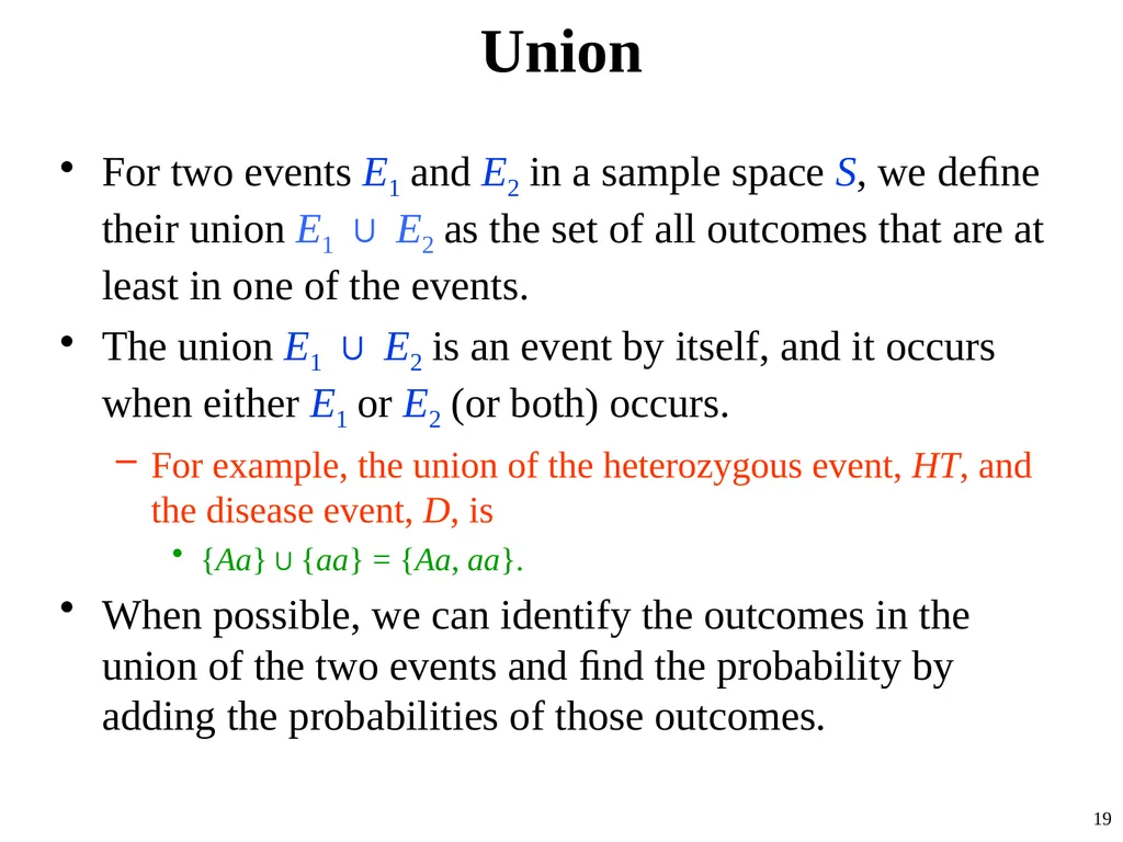
Union For two events E1 and E2 in a sample space S, we define their union E1 ∪ E2 as the set of all outcomes that are at least in one of the events.
The union E1 ∪ E2 is an event by itself, and it occurs when either E1 or E2 (or both) occurs.
For example, the union of the heterozygous event, HT, and the disease event, D, is
{Aa}∪{aa} = {Aa, aa}.
When possible, we can identify the outcomes in the union of the two events and find the probability by adding the probabilities of those outcomes. 19<br>
The union E1 ∪ E2 is an event by itself, and it occurs when either E1 or E2 (or both) occurs.
For example, the union of the heterozygous event, HT, and the disease event, D, is
{Aa}∪{aa} = {Aa, aa}.
When possible, we can identify the outcomes in the union of the two events and find the probability by adding the probabilities of those outcomes. 19<br>
20
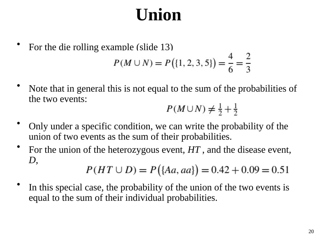
Union For the die rolling example (slide 13)
Note that in general this is not equal to the sum of the probabilities of the two events:
Only under a specific condition, we can write the probability of the union of two events as the sum of their probabilities.
For the union of the heterozygous event, HT , and the disease event, D,
In this special case, the probability of the union of the two events is equal to the sum of their individual probabilities. 20<br>
Note that in general this is not equal to the sum of the probabilities of the two events:
Only under a specific condition, we can write the probability of the union of two events as the sum of their probabilities.
For the union of the heterozygous event, HT , and the disease event, D,
In this special case, the probability of the union of the two events is equal to the sum of their individual probabilities. 20<br>
21
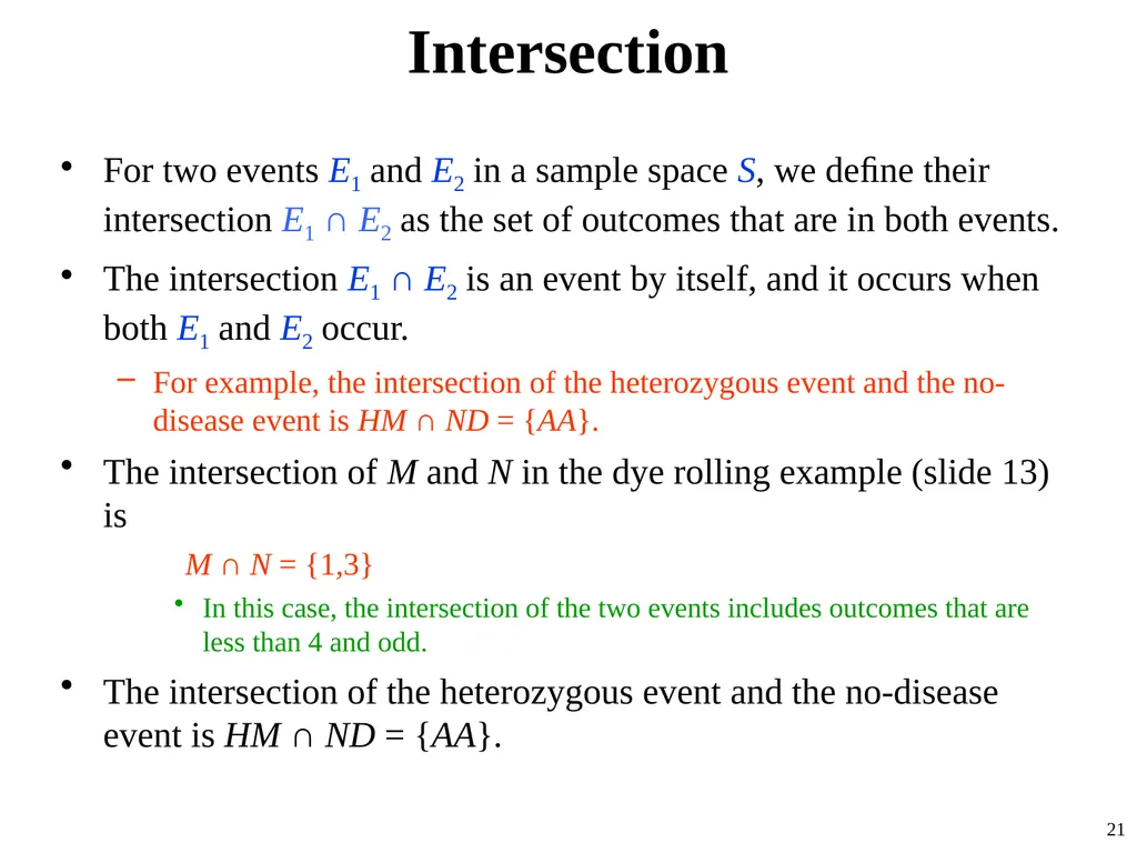
Intersection For two events E1 and E2 in a sample space S, we define their intersection E1 ∩ E2 as the set of outcomes that are in both events.
The intersection E1 ∩ E2 is an event by itself, and it occurs when both E1 and E2 occur.
For example, the intersection of the heterozygous event and the no-disease event is HM ∩ ND = {AA}.
The intersection of M and N in the dye rolling example (slide 13) is
M ∩ N = {1,3}
In this case, the intersection of the two events includes outcomes that are less than 4 and odd.
The intersection of the heterozygous event and the no-disease event is HM ∩ ND = {AA}. 21<br>
The intersection E1 ∩ E2 is an event by itself, and it occurs when both E1 and E2 occur.
For example, the intersection of the heterozygous event and the no-disease event is HM ∩ ND = {AA}.
The intersection of M and N in the dye rolling example (slide 13) is
M ∩ N = {1,3}
In this case, the intersection of the two events includes outcomes that are less than 4 and odd.
The intersection of the heterozygous event and the no-disease event is HM ∩ ND = {AA}. 21<br>
22
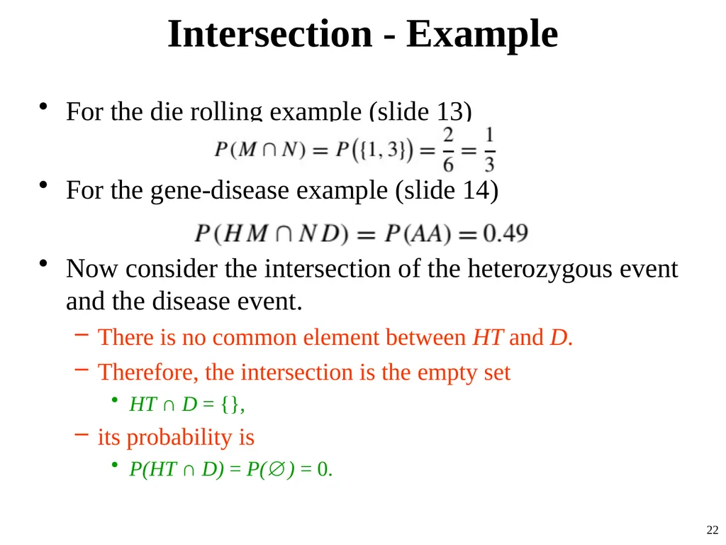
Intersection - Example For the die rolling example (slide 13)
For the gene-disease example (slide 14)
Now consider the intersection of the heterozygous event and the disease event.
There is no common element between HT and D.
Therefore, the intersection is the empty set
HT ∩ D = {},
its probability is
P(HT ∩ D) = P(∅) = 0. 22<br>
For the gene-disease example (slide 14)
Now consider the intersection of the heterozygous event and the disease event.
There is no common element between HT and D.
Therefore, the intersection is the empty set
HT ∩ D = {},
its probability is
P(HT ∩ D) = P(∅) = 0. 22<br>
23
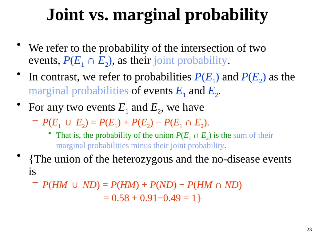
Joint vs. marginal probability We refer to the probability of the intersection of two events, P(E1 ∩ E2), as their joint probability.
In contrast, we refer to probabilities P(E1) and P(E2) as the marginal probabilities of events E1 and E2.
For any two events E1 and E2, we have
P(E1 ∪ E2) = P(E1) + P(E2) − P(E1 ∩ E2).
That is, the probability of the union P(E1 ∩ E2) is the sum of their marginal probabilities minus their joint probability.
{The union of the heterozygous and the no-disease events is
P(HM ∪ ND) = P(HM) + P(ND) − P(HM ∩ ND)
= 0.58 + 0.91−0.49 = 1} 23<br>
In contrast, we refer to probabilities P(E1) and P(E2) as the marginal probabilities of events E1 and E2.
For any two events E1 and E2, we have
P(E1 ∪ E2) = P(E1) + P(E2) − P(E1 ∩ E2).
That is, the probability of the union P(E1 ∩ E2) is the sum of their marginal probabilities minus their joint probability.
{The union of the heterozygous and the no-disease events is
P(HM ∪ ND) = P(HM) + P(ND) − P(HM ∩ ND)
= 0.58 + 0.91−0.49 = 1} 23<br>
24
Disjoint events Two events are called disjoint or mutually exclusive if they never occur together:
if we know that one of them has occurred, we can conclude that the other event has not.
Disjoint events have no elements (outcomes) in common, and their intersection is the empty set.
{For the above example (slide 14), if a person is heterozygous, we know that he does not have the disease
so the two events HT and ND are disjoint.} 24<br>
if we know that one of them has occurred, we can conclude that the other event has not.
Disjoint events have no elements (outcomes) in common, and their intersection is the empty set.
{For the above example (slide 14), if a person is heterozygous, we know that he does not have the disease
so the two events HT and ND are disjoint.} 24<br>
25
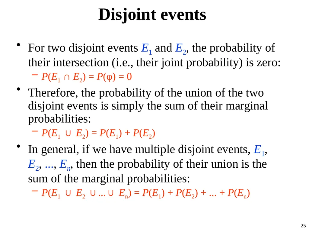
Disjoint events For two disjoint events E1 and E2, the probability of their intersection (i.e., their joint probability) is zero:
P(E1 ∩ E2) = P(φ) = 0
Therefore, the probability of the union of the two disjoint events is simply the sum of their marginal probabilities:
P(E1 ∪ E2) = P(E1) + P(E2)
In general, if we have multiple disjoint events, E1, E2, ..., En, then the probability of their union is the sum of the marginal probabilities:
P(E1 ∪ E2 ∪...∪ En) = P(E1) + P(E2) + ... + P(En) 25<br>
P(E1 ∩ E2) = P(φ) = 0
Therefore, the probability of the union of the two disjoint events is simply the sum of their marginal probabilities:
P(E1 ∪ E2) = P(E1) + P(E2)
In general, if we have multiple disjoint events, E1, E2, ..., En, then the probability of their union is the sum of the marginal probabilities:
P(E1 ∪ E2 ∪...∪ En) = P(E1) + P(E2) + ... + P(En) 25<br>
26
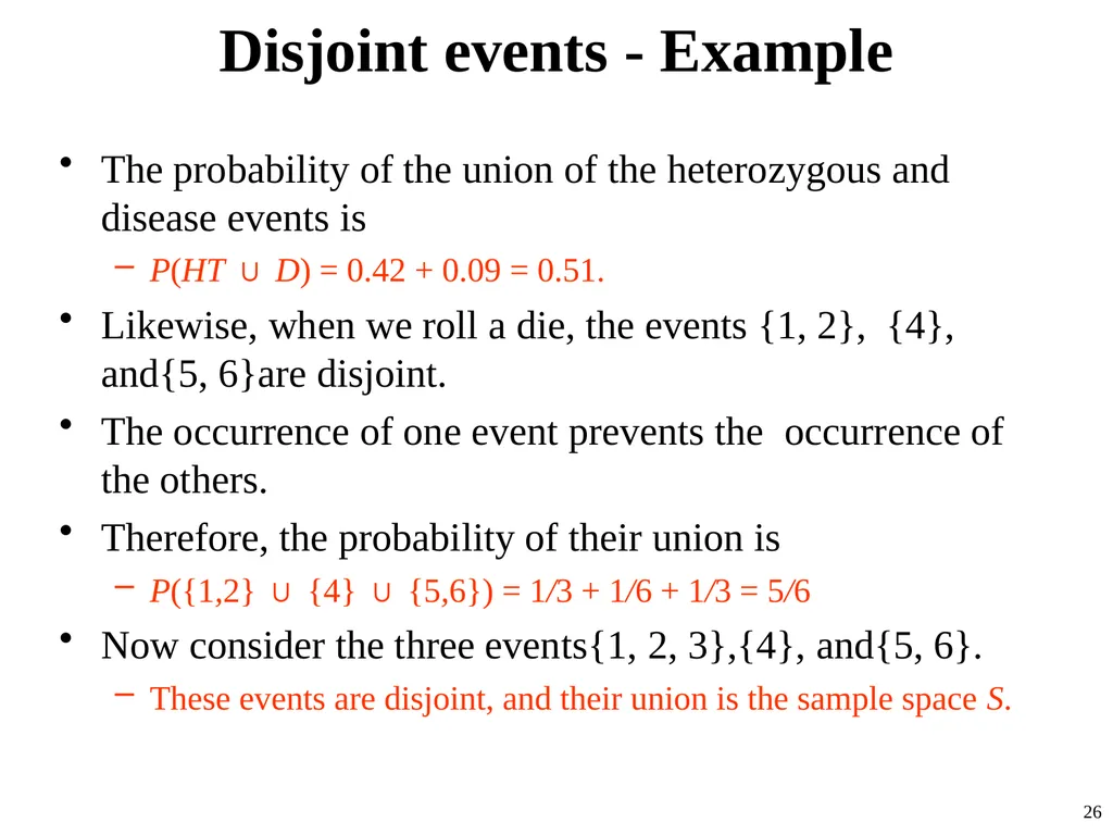
Disjoint events - Example The probability of the union of the heterozygous and disease events is
P(HT ∪ D) = 0.42 + 0.09 = 0.51.
Likewise, when we roll a die, the events {1, 2}, {4}, and{5, 6}are disjoint.
The occurrence of one event prevents the occurrence of the others.
Therefore, the probability of their union is
P({1,2} ∪ {4} ∪ {5,6}) = 1/3 + 1/6 + 1/3 = 5/6
Now consider the three events{1, 2, 3},{4}, and{5, 6}.
These events are disjoint, and their union is the sample space S. 26<br>
P(HT ∪ D) = 0.42 + 0.09 = 0.51.
Likewise, when we roll a die, the events {1, 2}, {4}, and{5, 6}are disjoint.
The occurrence of one event prevents the occurrence of the others.
Therefore, the probability of their union is
P({1,2} ∪ {4} ∪ {5,6}) = 1/3 + 1/6 + 1/3 = 5/6
Now consider the three events{1, 2, 3},{4}, and{5, 6}.
These events are disjoint, and their union is the sample space S. 26<br>
27
Partition When two or more events are disjoint and their union is the sample space S,
we say that the events form a partition of the sample space.
Two complementary events E and Ec always form a partition of the sample space
since they are disjoint and their union is the sample space. 27<br>
we say that the events form a partition of the sample space.
Two complementary events E and Ec always form a partition of the sample space
since they are disjoint and their union is the sample space. 27<br>
28
Conditional Probability Very often, we need to discuss possible changes in the
probability of one event based on our knowledge regarding the occurrence of another event.
The conditional probability, denoted P(E1|E2), is
the probability of event E1 given that another event E2 has occurred.
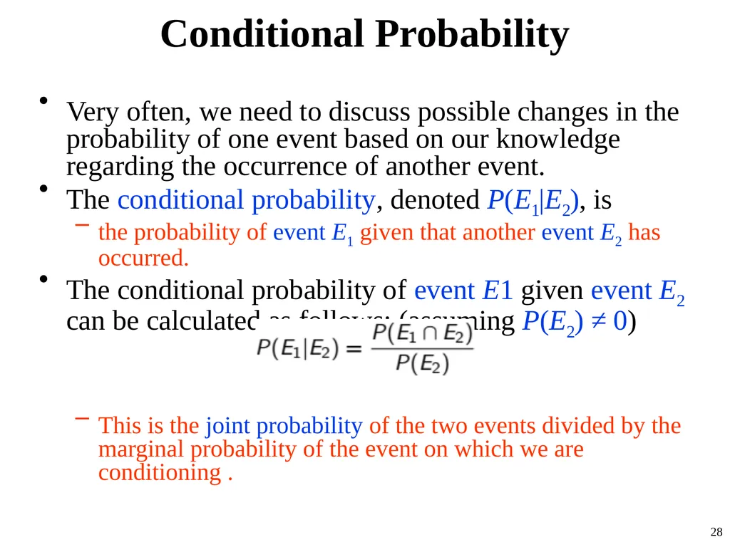
The conditional probability of event E1 given event E2 can be calculated as follows: (assuming P(E2) ≠ 0)
This is the joint probability of the two events divided by the marginal probability of the event on which we are conditioning . 28<br>
The conditional probability, denoted P(E1|E2), is
the probability of event E1 given that another event E2 has occurred.
The conditional probability of event E1 given event E2 can be calculated as follows: (assuming P(E2) ≠ 0)
This is the joint probability of the two events divided by the marginal probability of the event on which we are conditioning . 28<br>
29
Conditional Probability - Example Consider the die rolling example (slide 13).
The intersection of the two events is
M ∩ N = {1, 3}
with probability
P(E1 ∩ E2) = 2/6 = 1/3.
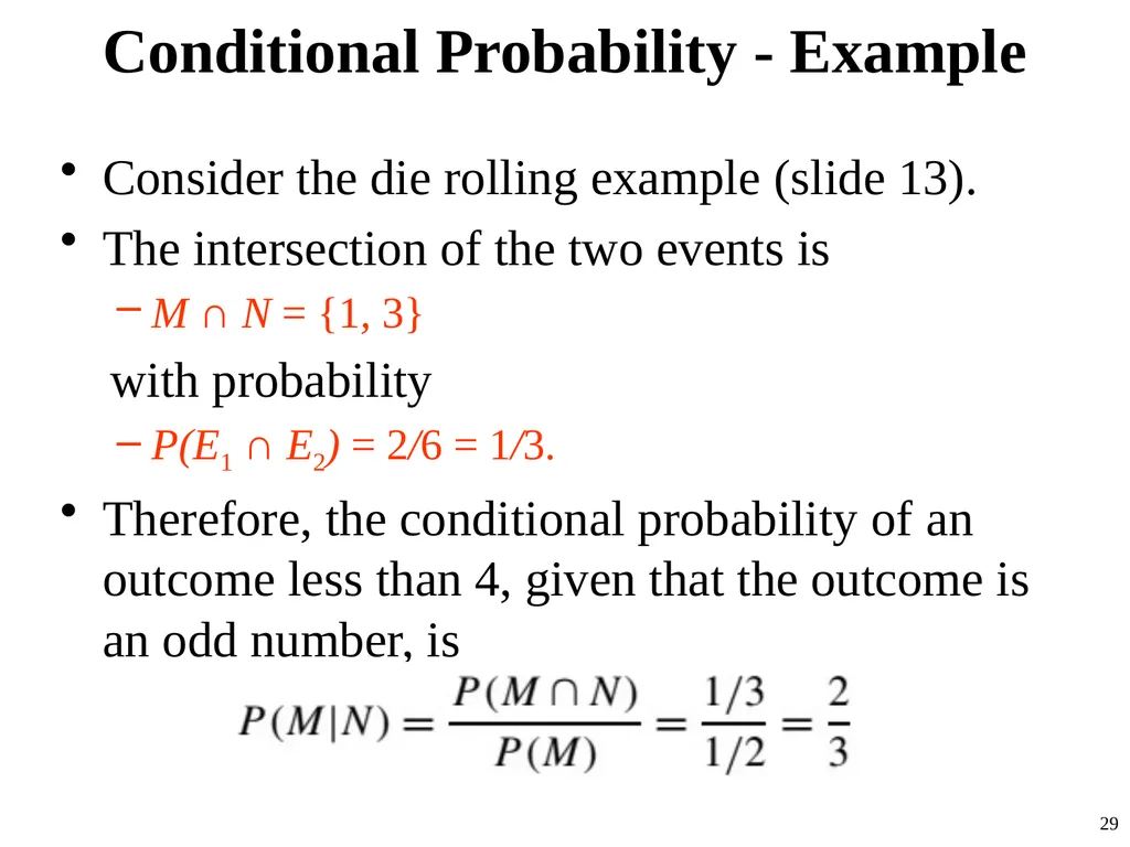
Therefore, the conditional probability of an outcome less than 4, given that the outcome is an odd number, is 29<br>
The intersection of the two events is
M ∩ N = {1, 3}
with probability
P(E1 ∩ E2) = 2/6 = 1/3.
Therefore, the conditional probability of an outcome less than 4, given that the outcome is an odd number, is 29<br>
30
Conditional Probability - Example Consider the gene-disease example (slide 14).
Suppose we know that a person is homozygous and are interested in the probability that this person has the disease, P(D|HM).
The probability of the intersection of D and HM is
P(D ∩ HM) = P({aa}) = 0.09
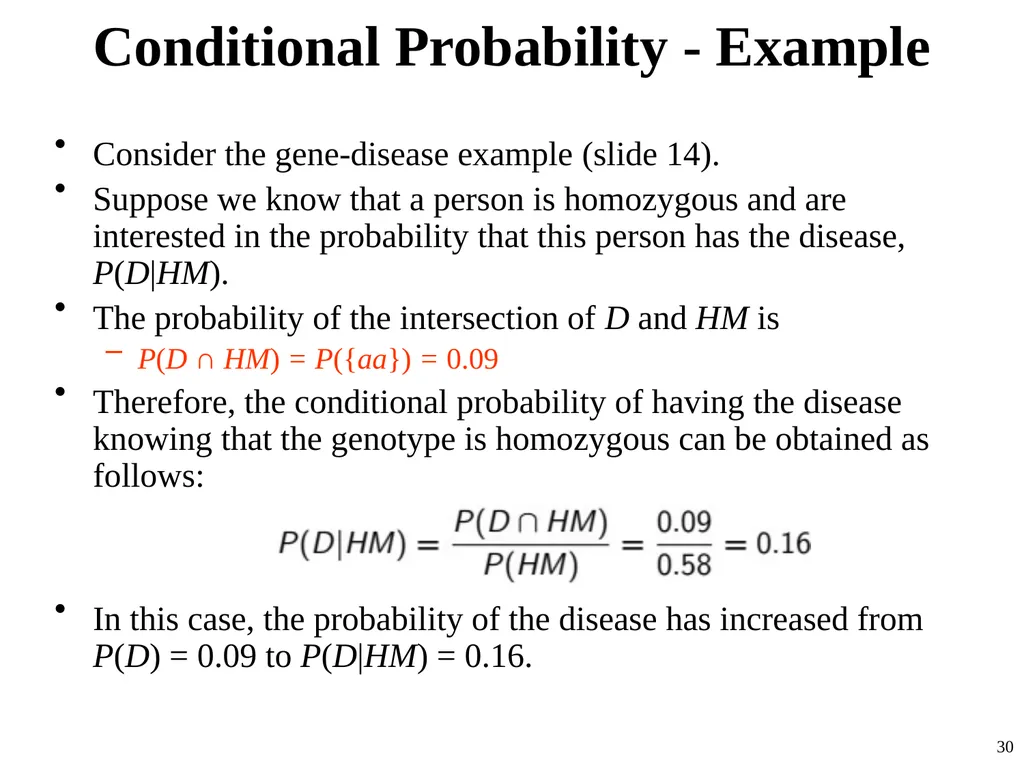
Therefore, the conditional probability of having the disease knowing that the genotype is homozygous can be obtained as follows:
In this case, the probability of the disease has increased from P(D) = 0.09 to P(D|HM) = 0.16. 30<br>
Suppose we know that a person is homozygous and are interested in the probability that this person has the disease, P(D|HM).
The probability of the intersection of D and HM is
P(D ∩ HM) = P({aa}) = 0.09
Therefore, the conditional probability of having the disease knowing that the genotype is homozygous can be obtained as follows:
In this case, the probability of the disease has increased from P(D) = 0.09 to P(D|HM) = 0.16. 30<br>
31
Conditional Probability - Example Now let us find the conditional probability of not having the disease knowing that the person has a homozygous genotype: P(ND|HM).
The joint probability of ND and HM is
P(ND ∩ HM) = P({AA}) = 0.49.
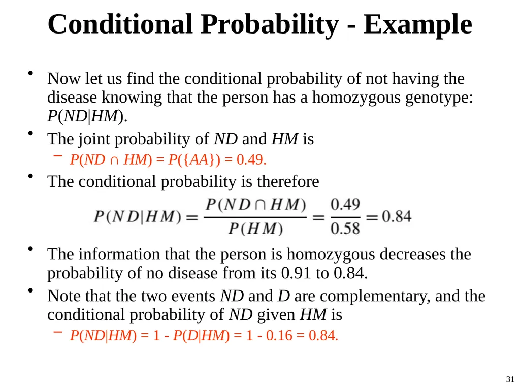
The conditional probability is therefore
The information that the person is homozygous decreases the probability of no disease from its 0.91 to 0.84.
Note that the two events ND and D are complementary, and the conditional probability of ND given HM is
P(ND|HM) = 1 - P(D|HM) = 1 - 0.16 = 0.84. 31<br>
The joint probability of ND and HM is
P(ND ∩ HM) = P({AA}) = 0.49.
The conditional probability is therefore
The information that the person is homozygous decreases the probability of no disease from its 0.91 to 0.84.
Note that the two events ND and D are complementary, and the conditional probability of ND given HM is
P(ND|HM) = 1 - P(D|HM) = 1 - 0.16 = 0.84. 31<br>
32
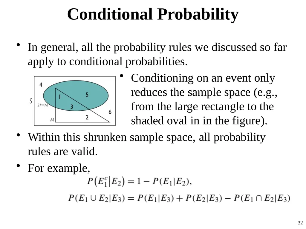
Conditional Probability In general, all the probability rules we discussed so far apply to conditional probabilities.
Conditioning on an event only reduces the sample space (e.g., from the large rectangle to the shaded oval in in the figure).
Within this shrunken sample space, all probability rules are valid.
For example, 32<br>
Conditioning on an event only reduces the sample space (e.g., from the large rectangle to the shaded oval in in the figure).
Within this shrunken sample space, all probability rules are valid.
For example, 32<br>
33
The law of total probability By rearranging the equation for conditional probabilities, we have
P(E1 ∩ E2) = P(E1|E2)P(E2).
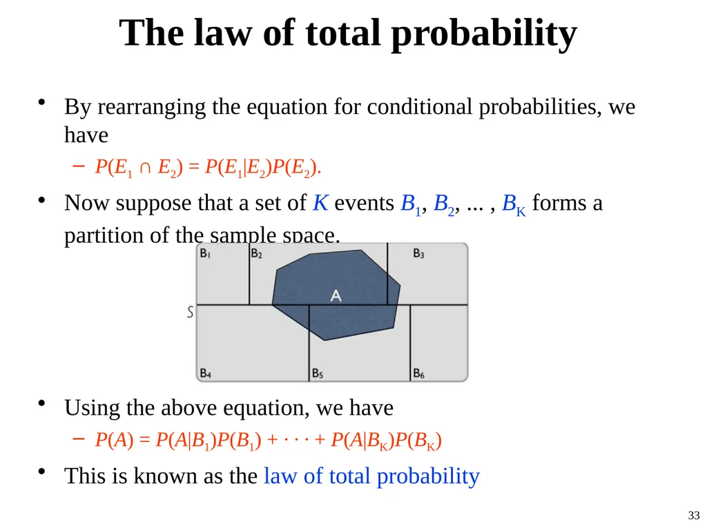
Now suppose that a set of K events B1, B2, ... , BK forms a partition of the sample space.
Using the above equation, we have
P(A) = P(A|B1)P(B1) + · · · + P(A|BK)P(BK)
This is known as the law of total probability 33<br>
P(E1 ∩ E2) = P(E1|E2)P(E2).
Now suppose that a set of K events B1, B2, ... , BK forms a partition of the sample space.
Using the above equation, we have
P(A) = P(A|B1)P(B1) + · · · + P(A|BK)P(BK)
This is known as the law of total probability 33<br>
34
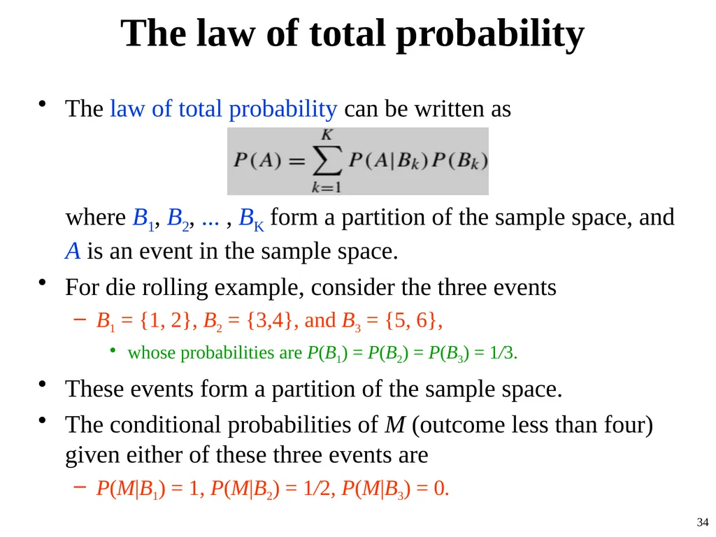
The law of total probability The law of total probability can be written as
where B1, B2, ... , BK form a partition of the sample space, and A is an event in the sample space.
For die rolling example, consider the three events
B1 = {1, 2}, B2 = {3,4}, and B3 = {5, 6},
whose probabilities are P(B1) = P(B2) = P(B3) = 1/3.
These events form a partition of the sample space.
The conditional probabilities of M (outcome less than four) given either of these three events are
P(M|B1) = 1, P(M|B2) = 1/2, P(M|B3) = 0. 34<br>
where B1, B2, ... , BK form a partition of the sample space, and A is an event in the sample space.
For die rolling example, consider the three events
B1 = {1, 2}, B2 = {3,4}, and B3 = {5, 6},
whose probabilities are P(B1) = P(B2) = P(B3) = 1/3.
These events form a partition of the sample space.
The conditional probabilities of M (outcome less than four) given either of these three events are
P(M|B1) = 1, P(M|B2) = 1/2, P(M|B3) = 0. 34<br>
35
The law of total probability If we know that the event B1 = {1, 2} has occurred, we know for sure that the outcome is less than 4.
Given B2 = {3, 4}, the possible outcomes are now 3 and 4.
One of two possible outcomes corresponds to the event M, that is, the conditional probability of M given B2 is 1/2.
If we know that the event B3 = {5, 6} has occurred,
then the probability that the number is less than 4 is zero: P(M|B3) = 0.
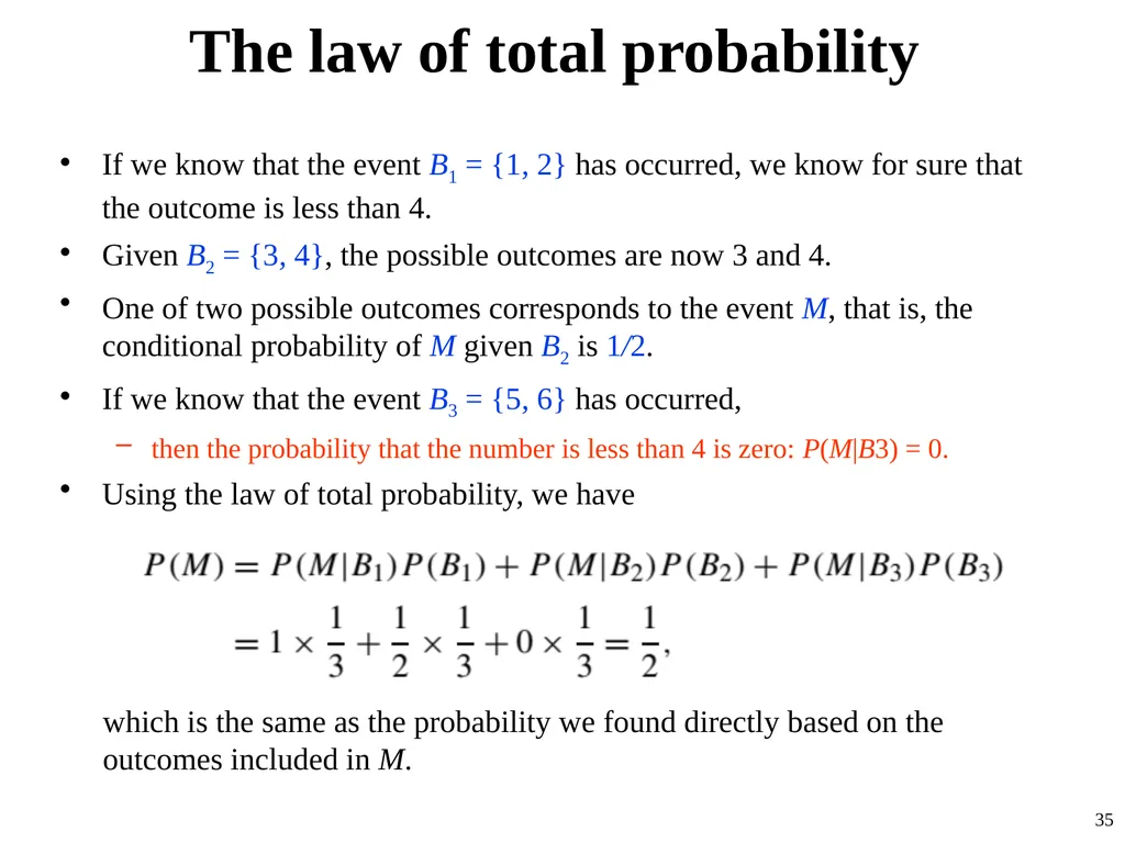
Using the law of total probability, we have
which is the same as the probability we found directly based on the outcomes included in M. 35<br>
Given B2 = {3, 4}, the possible outcomes are now 3 and 4.
One of two possible outcomes corresponds to the event M, that is, the conditional probability of M given B2 is 1/2.
If we know that the event B3 = {5, 6} has occurred,
then the probability that the number is less than 4 is zero: P(M|B3) = 0.
Using the law of total probability, we have
which is the same as the probability we found directly based on the outcomes included in M. 35<br>
36
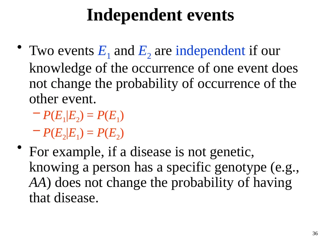
Independent events Two events E1 and E2 are independent if our knowledge of the occurrence of one event does not change the probability of occurrence of the other event.
P(E1|E2) = P(E1)
P(E2|E1) = P(E2)
For example, if a disease is not genetic, knowing a person has a specific genotype (e.g., AA) does not change the probability of having that disease. 36<br>
P(E1|E2) = P(E1)
P(E2|E1) = P(E2)
For example, if a disease is not genetic, knowing a person has a specific genotype (e.g., AA) does not change the probability of having that disease. 36<br>
37
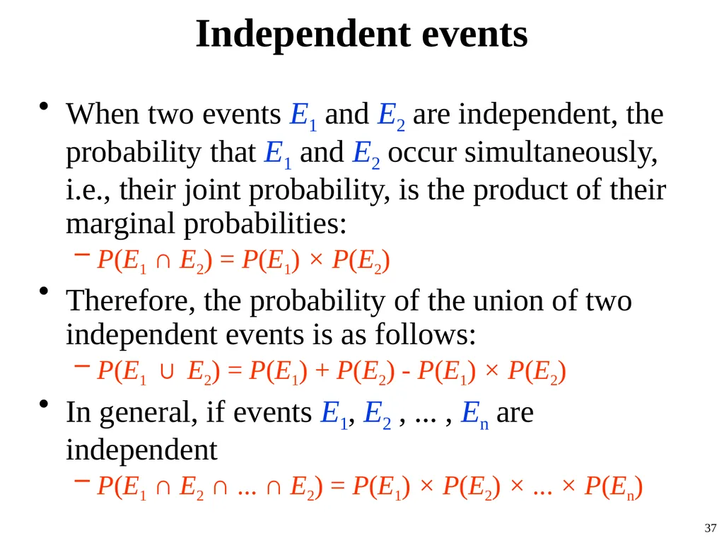
Independent events When two events E1 and E2 are independent, the probability that E1 and E2 occur simultaneously, i.e., their joint probability, is the product of their marginal probabilities:
P(E1 ∩ E2) = P(E1) × P(E2)
Therefore, the probability of the union of two independent events is as follows:
P(E1 ∪ E2) = P(E1) + P(E2) - P(E1) × P(E2)
In general, if events E1, E2 , ... , En are independent
P(E1 ∩ E2 ∩ ... ∩ E2) = P(E1) × P(E2) × ... × P(En) 37<br>
P(E1 ∩ E2) = P(E1) × P(E2)
Therefore, the probability of the union of two independent events is as follows:
P(E1 ∪ E2) = P(E1) + P(E2) - P(E1) × P(E2)
In general, if events E1, E2 , ... , En are independent
P(E1 ∩ E2 ∩ ... ∩ E2) = P(E1) × P(E2) × ... × P(En) 37<br>
38
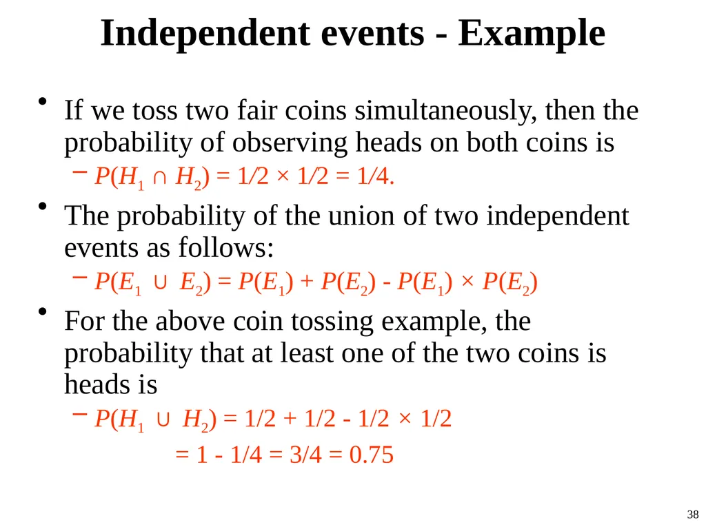
Independent events - Example If we toss two fair coins simultaneously, then the probability of observing heads on both coins is
P(H1 ∩ H2) = 1/2 × 1/2 = 1/4.
The probability of the union of two independent events as follows:
P(E1 ∪ E2) = P(E1) + P(E2) - P(E1) × P(E2)
For the above coin tossing example, the probability that at least one of the two coins is heads is
P(H1 ∪ H2) = 1/2 + 1/2 - 1/2 × 1/2
= 1 - 1/4 = 3/4 = 0.75 38<br>
P(H1 ∩ H2) = 1/2 × 1/2 = 1/4.
The probability of the union of two independent events as follows:
P(E1 ∪ E2) = P(E1) + P(E2) - P(E1) × P(E2)
For the above coin tossing example, the probability that at least one of the two coins is heads is
P(H1 ∪ H2) = 1/2 + 1/2 - 1/2 × 1/2
= 1 - 1/4 = 3/4 = 0.75 38<br>
39
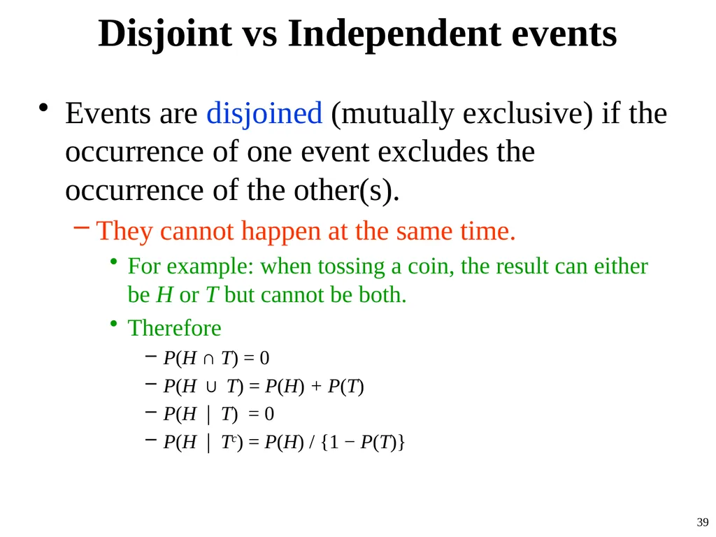
Disjoint vs Independent events Events are disjoined (mutually exclusive) if the occurrence of one event excludes the occurrence of the other(s).
They cannot happen at the same time.
For example: when tossing a coin, the result can either be H or T but cannot be both.
Therefore
P(H ∩ T) = 0
P(H ∪ T) = P(H) + P(T)
P(H ∣ T) = 0
P(H ∣ Tc) = P(H) / {1 − P(T)} 39<br>
They cannot happen at the same time.
For example: when tossing a coin, the result can either be H or T but cannot be both.
Therefore
P(H ∩ T) = 0
P(H ∪ T) = P(H) + P(T)
P(H ∣ T) = 0
P(H ∣ Tc) = P(H) / {1 − P(T)} 39<br>
40
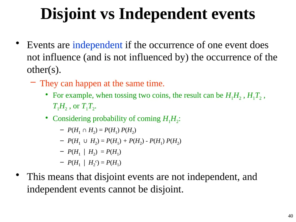
Disjoint vs Independent events Events are independent if the occurrence of one event does not influence (and is not influenced by) the occurrence of the other(s).
They can happen at the same time.
For example, when tossing two coins, the result can be H1H2 , H1T2 , T1H2 , or T1T2.
Considering probability of coming H1H2:
P(H1 ∩ H2) = P(H1) P(H2)
P(H1 ∪ H2) = P(H1) + P(H2) - P(H1) P(H2)
P(H1 ∣ H2) = P(H1)
P(H1 ∣ H2c) = P(H1)
This means that disjoint events are not independent, and independent events cannot be disjoint. 40<br>
They can happen at the same time.
For example, when tossing two coins, the result can be H1H2 , H1T2 , T1H2 , or T1T2.
Considering probability of coming H1H2:
P(H1 ∩ H2) = P(H1) P(H2)
P(H1 ∪ H2) = P(H1) + P(H2) - P(H1) P(H2)
P(H1 ∣ H2) = P(H1)
P(H1 ∣ H2c) = P(H1)
This means that disjoint events are not independent, and independent events cannot be disjoint. 40<br>
41
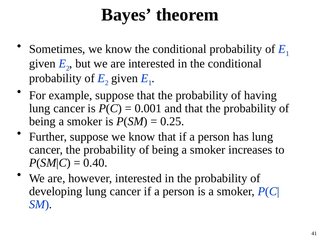
Bayes’ theorem Sometimes, we know the conditional probability of E1 given E2, but we are interested in the conditional probability of E2 given E1.
For example, suppose that the probability of having lung cancer is P(C) = 0.001 and that the probability of being a smoker is P(SM) = 0.25.
Further, suppose we know that if a person has lung cancer, the probability of being a smoker increases to P(SM|C) = 0.40.
We are, however, interested in the probability of developing lung cancer if a person is a smoker, P(C|SM). 41<br>
For example, suppose that the probability of having lung cancer is P(C) = 0.001 and that the probability of being a smoker is P(SM) = 0.25.
Further, suppose we know that if a person has lung cancer, the probability of being a smoker increases to P(SM|C) = 0.40.
We are, however, interested in the probability of developing lung cancer if a person is a smoker, P(C|SM). 41<br>
42
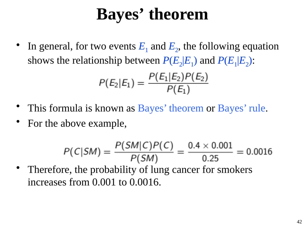
Bayes’ theorem In general, for two events E1 and E2, the following equation shows the relationship between P(E2|E1) and P(E1|E2):
This formula is known as Bayes’ theorem or Bayes’ rule.
For the above example,
Therefore, the probability of lung cancer for smokers increases from 0.001 to 0.0016. 42<br>
This formula is known as Bayes’ theorem or Bayes’ rule.
For the above example,
Therefore, the probability of lung cancer for smokers increases from 0.001 to 0.0016. 42<br>
43
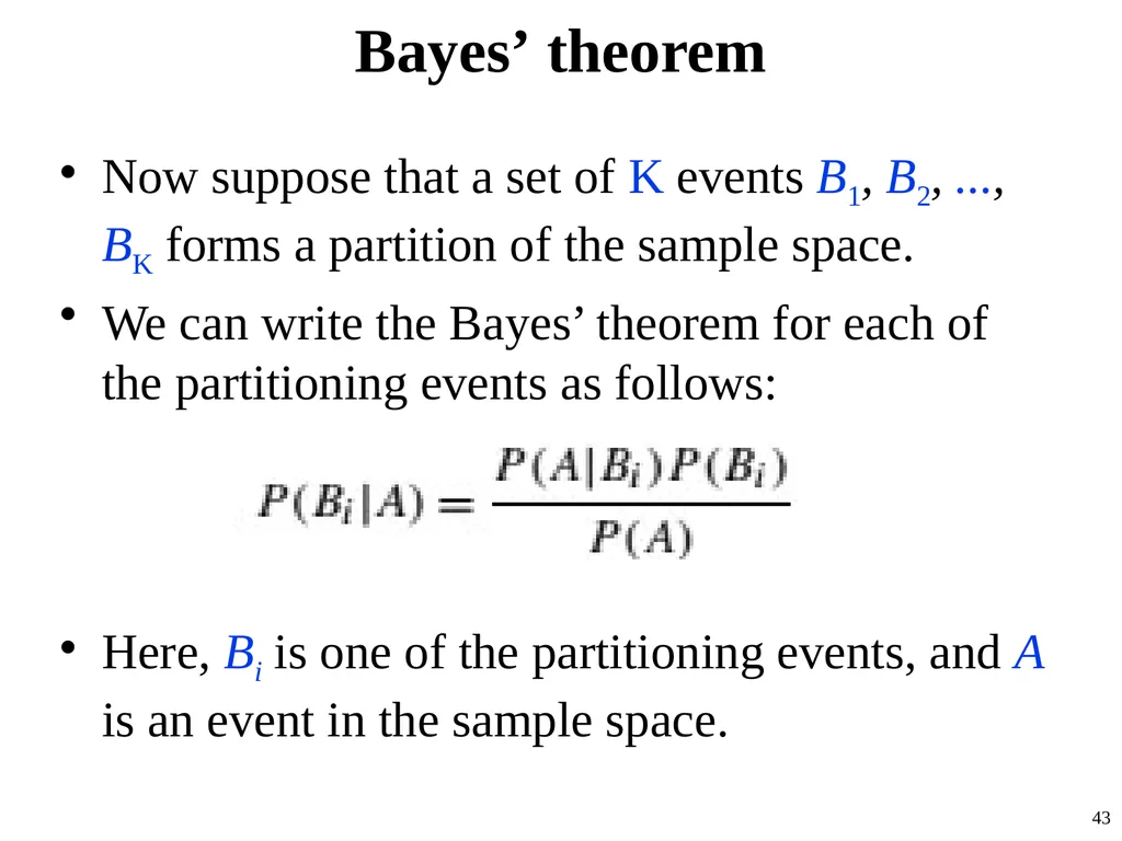
Bayes’ theorem Now suppose that a set of K events B1, B2, ..., BK forms a partition of the sample space.
We can write the Bayes’ theorem for each of the partitioning events as follows:
Here, Bi is one of the partitioning events, and A is an event in the sample space. 43<br>
We can write the Bayes’ theorem for each of the partitioning events as follows:
Here, Bi is one of the partitioning events, and A is an event in the sample space. 43<br>
44
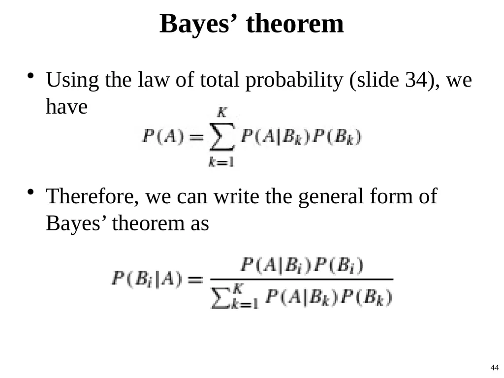
Bayes’ theorem Using the law of total probability (slide 34), we have
Therefore, we can write the general form of Bayes’ theorem as 44<br>
Therefore, we can write the general form of Bayes’ theorem as 44<br>
45
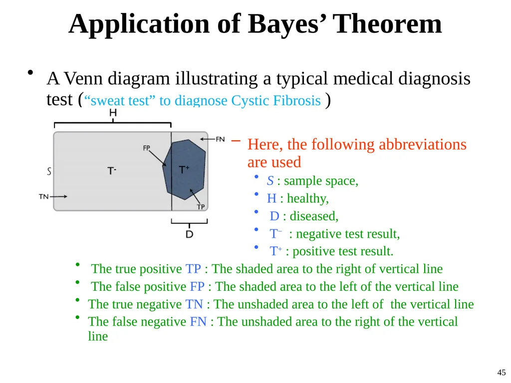
Application of Bayes’ Theorem A Venn diagram illustrating a typical medical diagnosis test (“sweat test” to diagnose Cystic Fibrosis )
Here, the following abbreviations are used
S : sample space,
H : healthy,
D : diseased,
T− : negative test result,
T+ : positive test result.
The true positive TP : The shaded area to the right of vertical line
The false positive FP : The shaded area to the left of the vertical line
The true negative TN : The unshaded area to the left of the vertical line
The false negative FN : The unshaded area to the right of the vertical line 45<br>
Here, the following abbreviations are used
S : sample space,
H : healthy,
D : diseased,
T− : negative test result,
T+ : positive test result.
The true positive TP : The shaded area to the right of vertical line
The false positive FP : The shaded area to the left of the vertical line
The true negative TN : The unshaded area to the left of the vertical line
The false negative FN : The unshaded area to the right of the vertical line 45<br>
46
Application of Bayes’ Theorem The sweat test is a simple procedure to detect CF by measuring the concentration of salt in a person’s sweat.
A high level of salt above a certain cutoff indicates CF.
The conditional probability of a positive diagnosis for CF patient, P(T+|D), is called the sensitivity of the test.
The conditional probability of a negative result for a healthy person, P(T−|H), is called the specificity of the test.
The probability of the CF disease for a child whose parents are both carriers is P(D) = 0.25.
Note that the gene causing CF is recessive.
Therefore, if we denote the allele causing CF as a and the normal allele as A, only people with aa genotype have CF.
People with Aa genotype are carriers.
If both parents are carriers, the chance of transmitting a is 0.5 for each parent 46<br>
A high level of salt above a certain cutoff indicates CF.
The conditional probability of a positive diagnosis for CF patient, P(T+|D), is called the sensitivity of the test.
The conditional probability of a negative result for a healthy person, P(T−|H), is called the specificity of the test.
The probability of the CF disease for a child whose parents are both carriers is P(D) = 0.25.
Note that the gene causing CF is recessive.
Therefore, if we denote the allele causing CF as a and the normal allele as A, only people with aa genotype have CF.
People with Aa genotype are carriers.
If both parents are carriers, the chance of transmitting a is 0.5 for each parent 46<br>
47
Application of Bayes’ Theorem Assuming that chromosomes from two parents are transmitted independently, there is the probability P(D) = 0.5×0.5 = 0.25 that the child becomes affected (i.e., aa genotype).
Then, the probability of being healthy is
P(H) = 1 − 0.25 = 0.75.
Assuming that the probability of false positive for the sweat test is P(T+|H) = 0.04 and the probability of false negative is P(T−|D) = 0.07
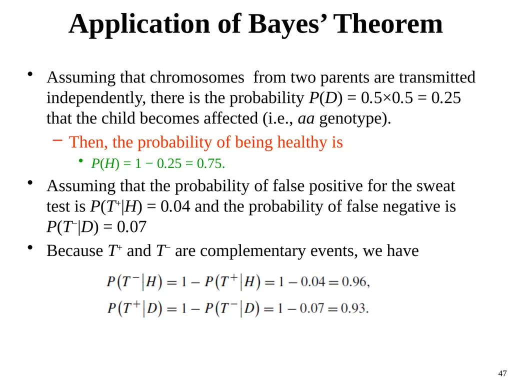
Because T+ and T− are complementary events, we have 47<br>
Then, the probability of being healthy is
P(H) = 1 − 0.25 = 0.75.
Assuming that the probability of false positive for the sweat test is P(T+|H) = 0.04 and the probability of false negative is P(T−|D) = 0.07
Because T+ and T− are complementary events, we have 47<br>
48
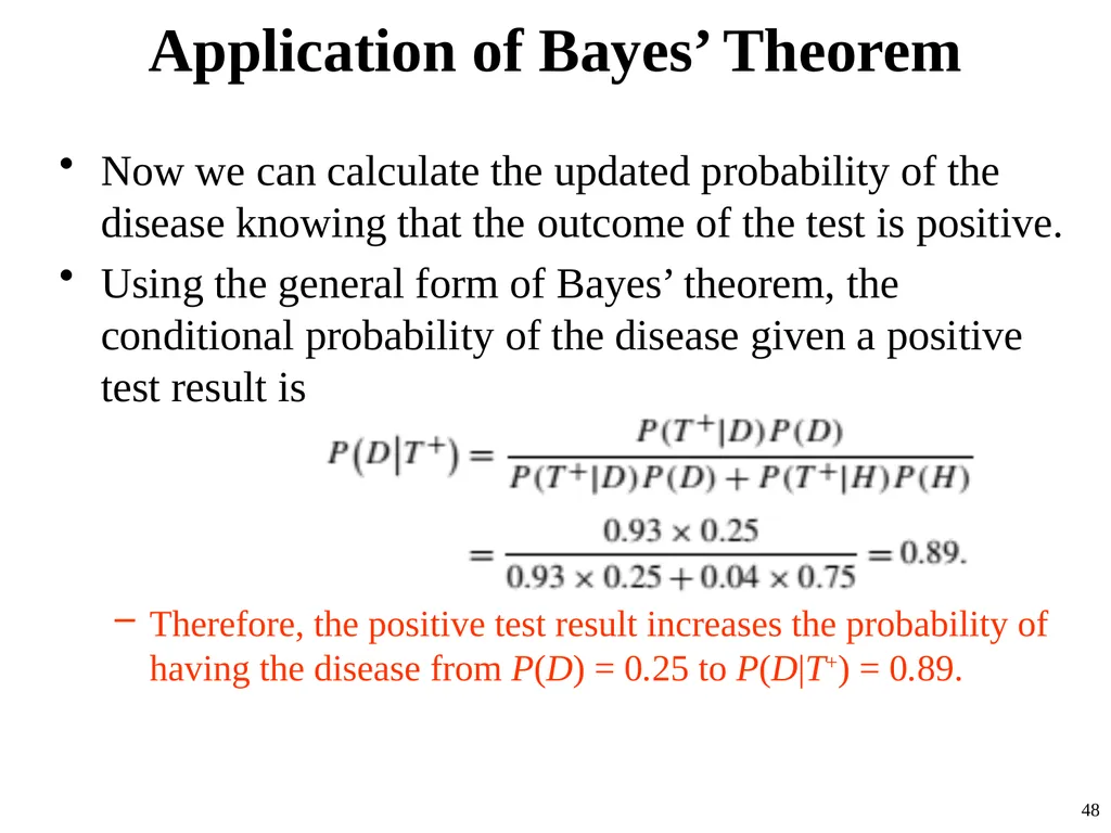
Application of Bayes’ Theorem Now we can calculate the updated probability of the disease knowing that the outcome of the test is positive.
Using the general form of Bayes’ theorem, the conditional probability of the disease given a positive test result is
Therefore, the positive test result increases the probability of having the disease from P(D) = 0.25 to P(D|T+) = 0.89. 48<br>
Using the general form of Bayes’ theorem, the conditional probability of the disease given a positive test result is
Therefore, the positive test result increases the probability of having the disease from P(D) = 0.25 to P(D|T+) = 0.89. 48<br>
49
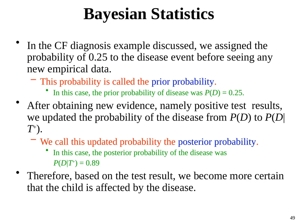
Bayesian Statistics In the CF diagnosis example discussed, we assigned the probability of 0.25 to the disease event before seeing any new empirical data.
This probability is called the prior probability.
In this case, the prior probability of disease was P(D) = 0.25.
After obtaining new evidence, namely positive test results, we updated the probability of the disease from P(D) to P(D|T+).
We call this updated probability the posterior probability.
In this case, the posterior probability of the disease was
P(D|T+) = 0.89
Therefore, based on the test result, we become more certain that the child is affected by the disease. 49<br>
This probability is called the prior probability.
In this case, the prior probability of disease was P(D) = 0.25.
After obtaining new evidence, namely positive test results, we updated the probability of the disease from P(D) to P(D|T+).
We call this updated probability the posterior probability.
In this case, the posterior probability of the disease was
P(D|T+) = 0.89
Therefore, based on the test result, we become more certain that the child is affected by the disease. 49<br>
50
Interpretation of Probability as the Relative Frequency The random phenomena we have been discussing so far can be observed repeatedly.
A coin can be tossed or a die can be rolled many times.
We can observe the genotypes of many people.
These repeated experiments or observations are called trials.
For such random phenomena, the probability of an event can be interpreted in terms of the relative frequency.
The above view of probability is the basis of Frequentist Statistics 50<br>
A coin can be tossed or a die can be rolled many times.
We can observe the genotypes of many people.
These repeated experiments or observations are called trials.
For such random phenomena, the probability of an event can be interpreted in terms of the relative frequency.
The above view of probability is the basis of Frequentist Statistics 50<br>
51
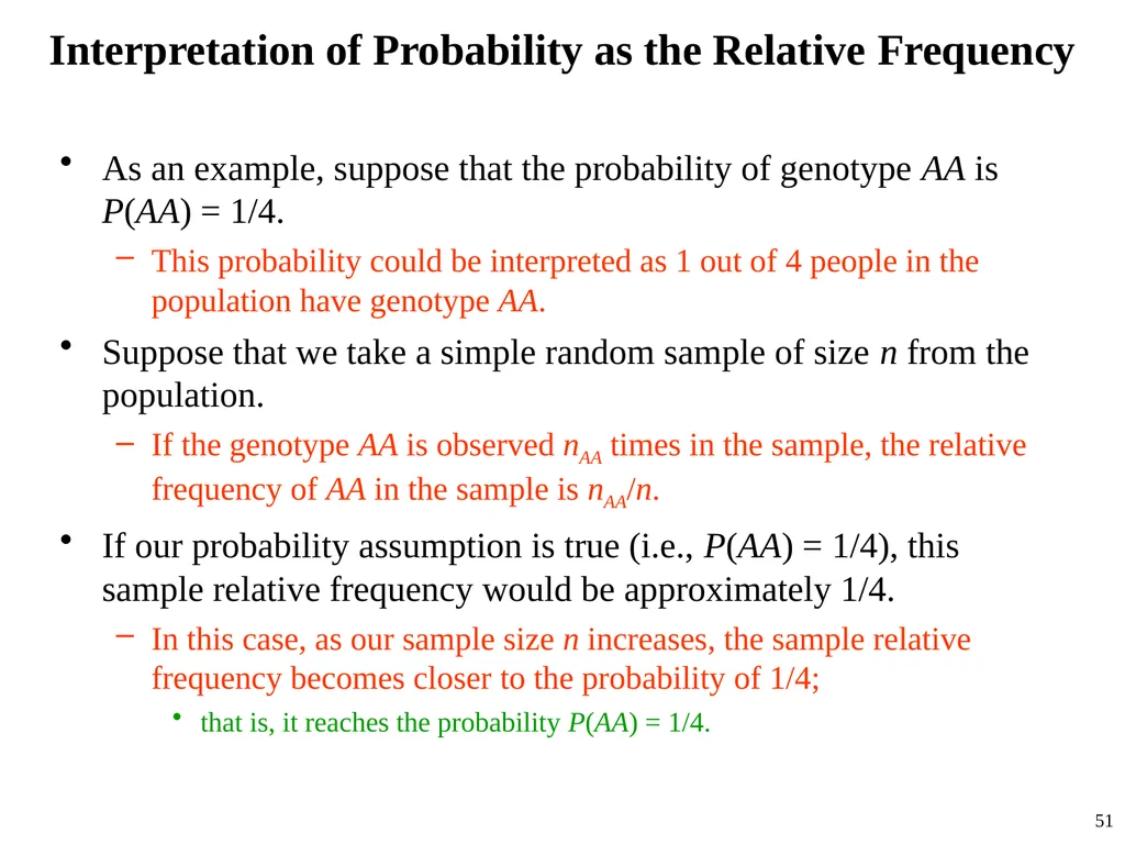
Interpretation of Probability as the Relative Frequency As an example, suppose that the probability of genotype AA is P(AA) = 1/4.
This probability could be interpreted as 1 out of 4 people in the population have genotype AA.
Suppose that we take a simple random sample of size n from the population.
If the genotype AA is observed nAA times in the sample, the relative frequency of AA in the sample is nAA/n.
If our probability assumption is true (i.e., P(AA) = 1/4), this sample relative frequency would be approximately 1/4.
In this case, as our sample size n increases, the sample relative frequency becomes closer to the probability of 1/4;
that is, it reaches the probability P(AA) = 1/4. 51<br>
This probability could be interpreted as 1 out of 4 people in the population have genotype AA.
Suppose that we take a simple random sample of size n from the population.
If the genotype AA is observed nAA times in the sample, the relative frequency of AA in the sample is nAA/n.
If our probability assumption is true (i.e., P(AA) = 1/4), this sample relative frequency would be approximately 1/4.
In this case, as our sample size n increases, the sample relative frequency becomes closer to the probability of 1/4;
that is, it reaches the probability P(AA) = 1/4. 51<br>
52
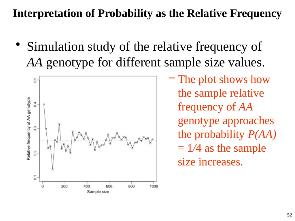
Interpretation of Probability as the Relative Frequency Simulation study of the relative frequency of AA genotype for different sample size values.
The plot shows how the sample relative frequency of AA genotype approaches the probability P(AA) = 1/4 as the sample size increases. 52<br>
The plot shows how the sample relative frequency of AA genotype approaches the probability P(AA) = 1/4 as the sample size increases. 52<br>
53
Interpretation of Probability as the Relative Frequency Note that the above interpretation of probability requires two important assumptions.
We assume that the probability of events does not change from one trial to another.
For example, the probability of AA must remain 1/4.
If the population changes as we are sampling people (e.g., genotype AA becomes more prevalent), then the sample relative frequency will not converge to 1/4.
We also assume that the outcome of one trial does not affect the outcome of another trial. 53<br>
We assume that the probability of events does not change from one trial to another.
For example, the probability of AA must remain 1/4.
If the population changes as we are sampling people (e.g., genotype AA becomes more prevalent), then the sample relative frequency will not converge to 1/4.
We also assume that the outcome of one trial does not affect the outcome of another trial. 53<br>
54
Using Tree Diagrams to Obtain Joint Probabilities Previously, we used tree diagrams to find the sample space for the combination of two random phenomena.
Tree diagrams can also be used for calculating their joint probabilities.
As an example, assume that the alleles on the homologous chromosomes are independent
i.e., the allele inherited from the mother has no influence on the allele inherited from the father.
Also assume that for a biallelic gene A, the allele probabilities are P(A) = 0.7 and P(a) = 0.3.
Then to find the genotype probabilities, we can use the tree diagram (shown in next slide). 54<br>
Tree diagrams can also be used for calculating their joint probabilities.
As an example, assume that the alleles on the homologous chromosomes are independent
i.e., the allele inherited from the mother has no influence on the allele inherited from the father.
Also assume that for a biallelic gene A, the allele probabilities are P(A) = 0.7 and P(a) = 0.3.
Then to find the genotype probabilities, we can use the tree diagram (shown in next slide). 54<br>
55
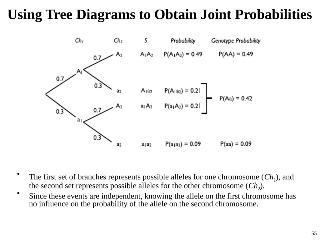
Using Tree Diagrams to Obtain Joint Probabilities The first set of branches represents possible alleles for one chromosome (Ch1), and the second set represents possible alleles for the other chromosome (Ch2).
Since these events are independent, knowing the allele on the first chromosome has no influence on the probability of the allele on the second chromosome. 55<br>
Since these events are independent, knowing the allele on the first chromosome has no influence on the probability of the allele on the second chromosome. 55<br>
56
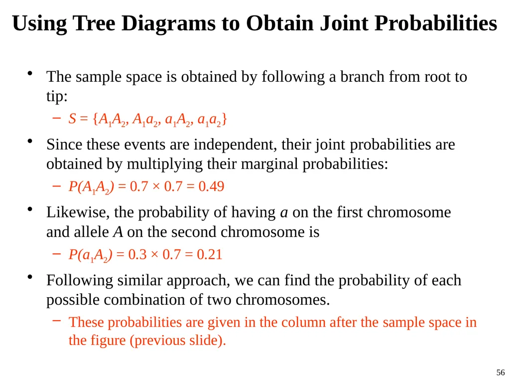
Using Tree Diagrams to Obtain Joint Probabilities The sample space is obtained by following a branch from root to tip:
S = {A1A2, A1a2, a1A2, a1a2}
Since these events are independent, their joint probabilities are obtained by multiplying their marginal probabilities:
P(A1A2) = 0.7 × 0.7 = 0.49
Likewise, the probability of having a on the first chromosome and allele A on the second chromosome is
P(a1A2) = 0.3 × 0.7 = 0.21
Following similar approach, we can find the probability of each possible combination of two chromosomes.
These probabilities are given in the column after the sample space in the figure (previous slide). 56<br>
S = {A1A2, A1a2, a1A2, a1a2}
Since these events are independent, their joint probabilities are obtained by multiplying their marginal probabilities:
P(A1A2) = 0.7 × 0.7 = 0.49
Likewise, the probability of having a on the first chromosome and allele A on the second chromosome is
P(a1A2) = 0.3 × 0.7 = 0.21
Following similar approach, we can find the probability of each possible combination of two chromosomes.
These probabilities are given in the column after the sample space in the figure (previous slide). 56<br>
57
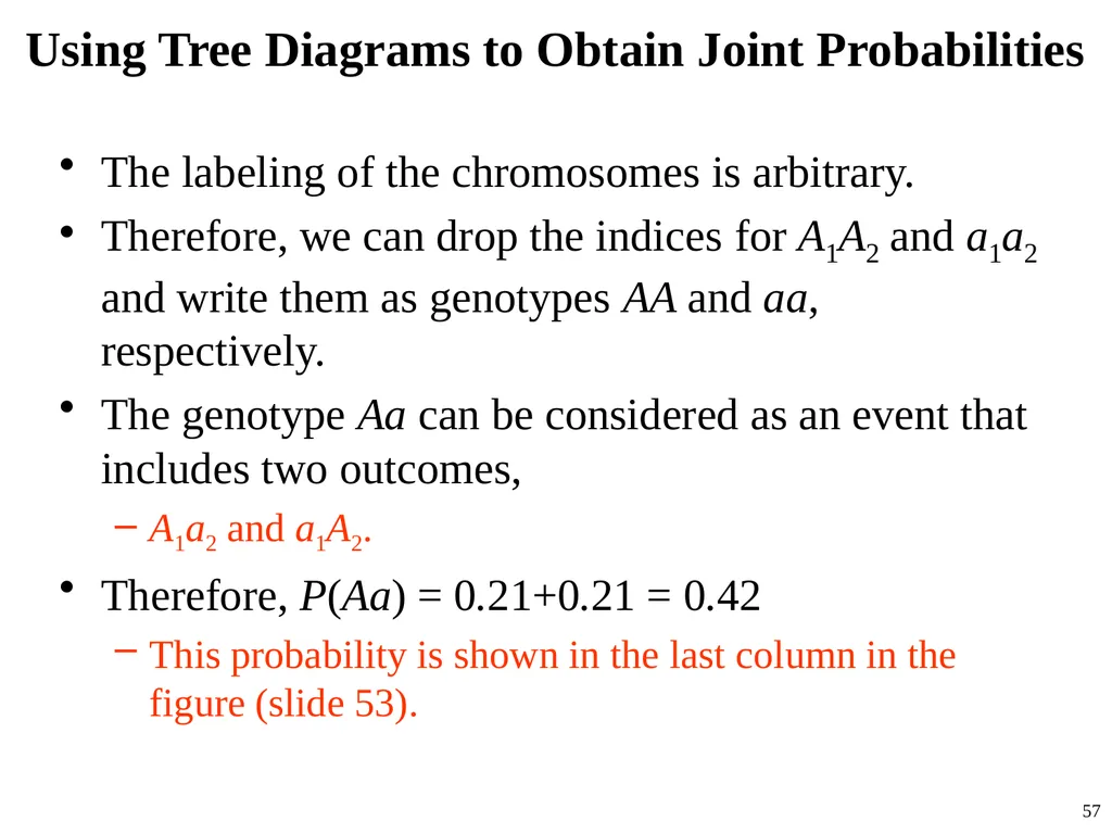
Using Tree Diagrams to Obtain Joint Probabilities The labeling of the chromosomes is arbitrary.
Therefore, we can drop the indices for A1A2 and a1a2 and write them as genotypes AA and aa, respectively.
The genotype Aa can be considered as an event that includes two outcomes,
A1a2 and a1A2.
Therefore, P(Aa) = 0.21+0.21 = 0.42
This probability is shown in the last column in the figure (slide 53). 57<br>
Therefore, we can drop the indices for A1A2 and a1a2 and write them as genotypes AA and aa, respectively.
The genotype Aa can be considered as an event that includes two outcomes,
A1a2 and a1A2.
Therefore, P(Aa) = 0.21+0.21 = 0.42
This probability is shown in the last column in the figure (slide 53). 57<br>
58
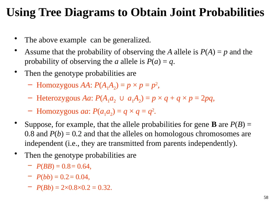
Using Tree Diagrams to Obtain Joint Probabilities The above example can be generalized.
Assume that the probability of observing the A allele is P(A) = p and the probability of observing the a allele is P(a) = q.
Then the genotype probabilities are
Homozygous AA: P(A1A2) = p × p = p2,
Heterozygous Aa: P(A1a2 ∪ a1A2) = p × q + q × p = 2pq,
Homozygous aa: P(a1a2) = q × q = q2.
Suppose, for example, that the allele probabilities for gene B are P(B) = 0.8 and P(b) = 0.2 and that the alleles on homologous chromosomes are independent (i.e., they are transmitted from parents independently).
Then the genotype probabilities are
P(BB) = 0.82 = 0.64,
P(bb) = 0.22 = 0.04,
P(Bb) = 2×0.8×0.2 = 0.32. 58<br>
Assume that the probability of observing the A allele is P(A) = p and the probability of observing the a allele is P(a) = q.
Then the genotype probabilities are
Homozygous AA: P(A1A2) = p × p = p2,
Heterozygous Aa: P(A1a2 ∪ a1A2) = p × q + q × p = 2pq,
Homozygous aa: P(a1a2) = q × q = q2.
Suppose, for example, that the allele probabilities for gene B are P(B) = 0.8 and P(b) = 0.2 and that the alleles on homologous chromosomes are independent (i.e., they are transmitted from parents independently).
Then the genotype probabilities are
P(BB) = 0.82 = 0.64,
P(bb) = 0.22 = 0.04,
P(Bb) = 2×0.8×0.2 = 0.32. 58<br>
59
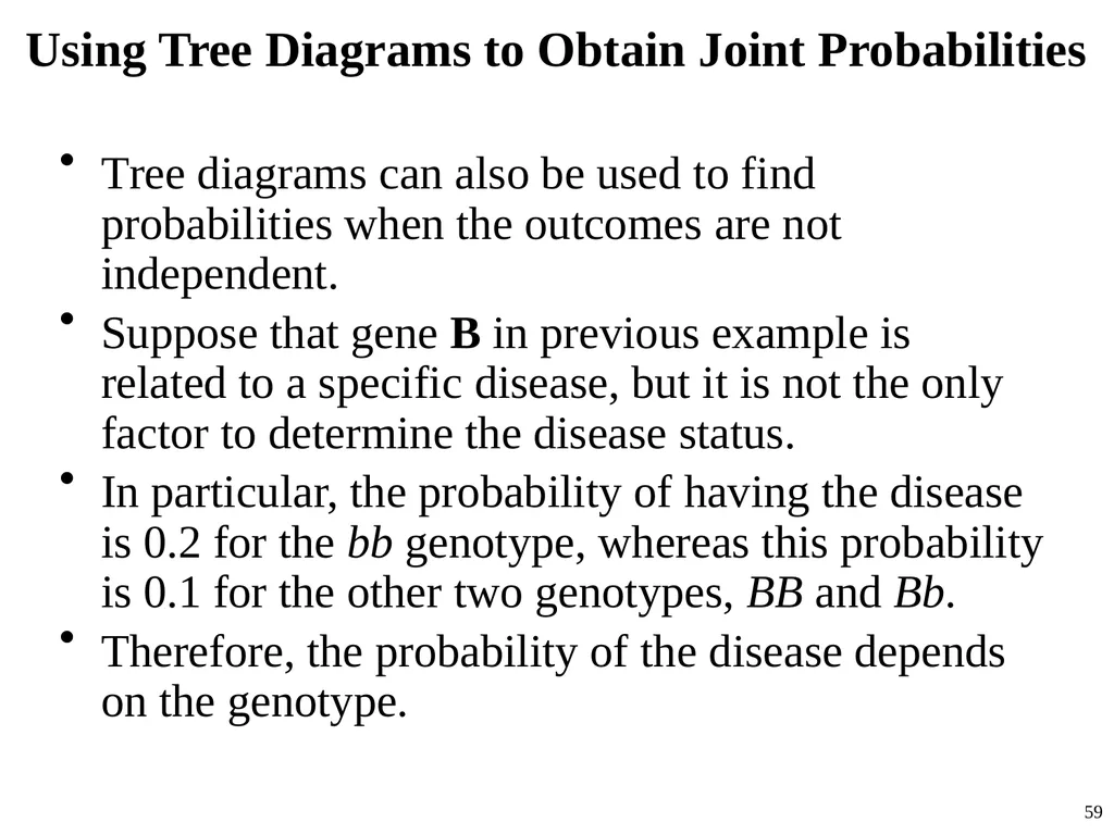
Using Tree Diagrams to Obtain Joint Probabilities Tree diagrams can also be used to find probabilities when the outcomes are not independent.
Suppose that gene B in previous example is related to a specific disease, but it is not the only factor to determine the disease status.
In particular, the probability of having the disease is 0.2 for the bb genotype, whereas this probability is 0.1 for the other two genotypes, BB and Bb.
Therefore, the probability of the disease depends on the genotype. 59<br>
Suppose that gene B in previous example is related to a specific disease, but it is not the only factor to determine the disease status.
In particular, the probability of having the disease is 0.2 for the bb genotype, whereas this probability is 0.1 for the other two genotypes, BB and Bb.
Therefore, the probability of the disease depends on the genotype. 59<br>
60
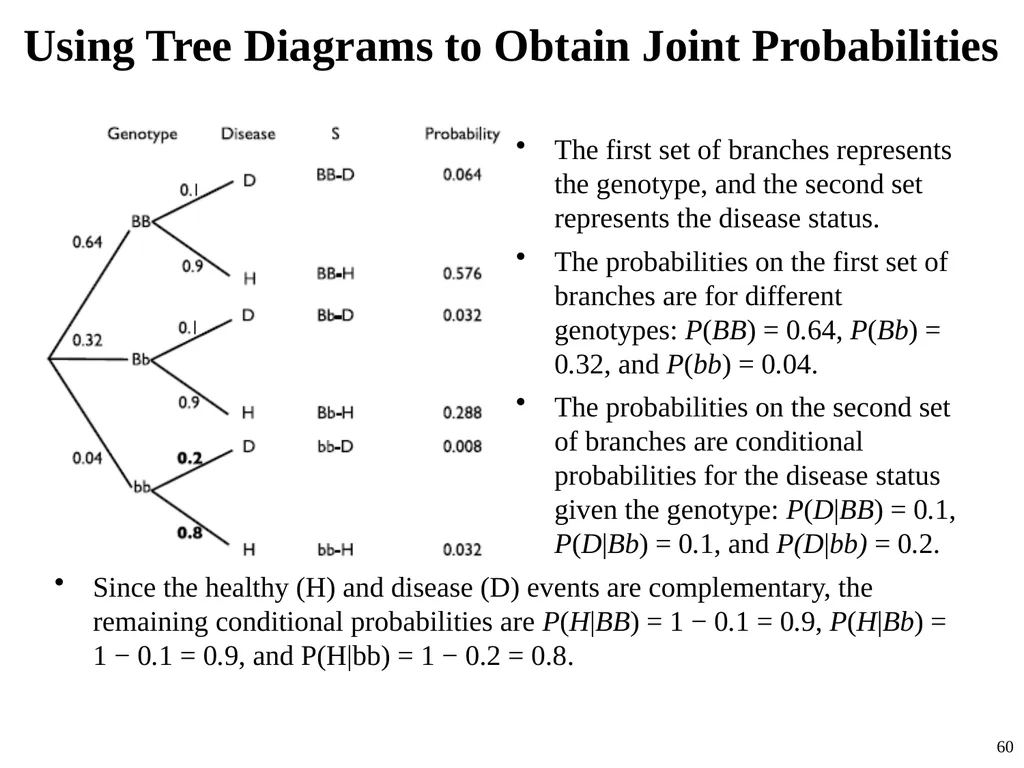
Using Tree Diagrams to Obtain Joint Probabilities The first set of branches represents the genotype, and the second set represents the disease status.
The probabilities on the first set of branches are for different genotypes: P(BB) = 0.64, P(Bb) = 0.32, and P(bb) = 0.04.
The probabilities on the second set of branches are conditional probabilities for the disease status given the genotype: P(D|BB) = 0.1, P(D|Bb) = 0.1, and P(D|bb) = 0.2.
Since the healthy (H) and disease (D) events are complementary, the remaining conditional probabilities are P(H|BB) = 1 − 0.1 = 0.9, P(H|Bb) = 1 − 0.1 = 0.9, and P(H|bb) = 1 − 0.2 = 0.8. 60<br>
The probabilities on the first set of branches are for different genotypes: P(BB) = 0.64, P(Bb) = 0.32, and P(bb) = 0.04.
The probabilities on the second set of branches are conditional probabilities for the disease status given the genotype: P(D|BB) = 0.1, P(D|Bb) = 0.1, and P(D|bb) = 0.2.
Since the healthy (H) and disease (D) events are complementary, the remaining conditional probabilities are P(H|BB) = 1 − 0.1 = 0.9, P(H|Bb) = 1 − 0.1 = 0.9, and P(H|bb) = 1 − 0.2 = 0.8. 60<br>
61
Using Tree Diagrams to Obtain Joint Probabilities Unlike the tree for independent events, the probabilities on the second set of branches depend on the outcomes on the first set of branches.
As before, we follow the branches from the root to tip and obtain the sample space:
S = {BB − D, BB − H, Bb − D, Bb − H, bb − D, bb − H}.
To find their probabilities, which are in fact the joint probabilities of genotype and disease status, we multiply the probabilities on the corresponding branches.
For example, the probability of Bb − D is the product of the conditional probability P(D|Bb) and the marginal probability P(Bb):
P(Bb −D) = P(Bb)P (D|Bb) = 0.32 × 0.1 = 0.032. 61<br>
As before, we follow the branches from the root to tip and obtain the sample space:
S = {BB − D, BB − H, Bb − D, Bb − H, bb − D, bb − H}.
To find their probabilities, which are in fact the joint probabilities of genotype and disease status, we multiply the probabilities on the corresponding branches.
For example, the probability of Bb − D is the product of the conditional probability P(D|Bb) and the marginal probability P(Bb):
P(Bb −D) = P(Bb)P (D|Bb) = 0.32 × 0.1 = 0.032. 61<br>
62
62<br>