
Statistical Process Control (SPC) Training Guide
LD
Published · 61 slides · 0 views

1 / 1

Description
Statistical Process Control (SPC) Training Guide What is data? Data is factual information (as measurements or statistics) used as a basic for reasoning, discussion or calculation. (Merriam-Webster Dictionary, m-w.com) What does this mean?
Related Topics
Share
Embed code
Download this presentation From Below
"Statistical Process Control (SPC) Training Guide" is the property of its rightful owner. Permission is granted to download and print the materials on this website for personal, non-commercial use only, and to display it on your personal computer provided you do not modify the materials and that you retain all copyright notices contained in the materials. By downloading content from our website, you accept the terms of this agreement.
Presentation Transcript
01
Statistical Process Control (SPC)
Training Guide<br>
Training Guide<br>
02
What is data? Data is factual information (as measurements or statistics) used as a basic for reasoning, discussion or calculation. (Merriam-Webster Dictionary, m-w.com)
What does this mean?
Data allows us to make educated decisions and take action!<br>
What does this mean?
Data allows us to make educated decisions and take action!<br>
03
Why is Data Important? If we don’t collect data about a process then what?
Without data we don’t understand the process / product
So what?
Without understanding of the process / product we can’t control the outcome
Is it important to control the outcome?
When you can’t control the outcome you are dependent on chance.
You may have a good outcome, you may not.
Without data collection you may not know either way.<br>
04
Use of Data I’m not collecting data because its non value add.
Without data collection there is no way to identify problems, continuously improve or ensure you are meeting the voice of the customer.
I’m collecting data, but not looking at it. Is that okay?
No, the collection of data without analysis is a bigger waste than not collecting data in the first place.
What should I be doing with the data?<br>
05
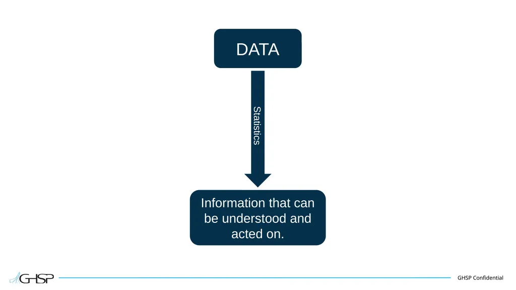
DATA Statistics Information that can be understood and acted on.<br>
06
What are Statistics A branch of mathematics dealing with the collection, analysis, interpretation and presentation of masses of numerical data (Merriam-Webster Dictionary, m-w.com)
What does this mean?
Once data is collected we can use appropriate statistical methods to describe (understand) our process / product and control (predict) the process / product outcome<br>
What does this mean?
Once data is collected we can use appropriate statistical methods to describe (understand) our process / product and control (predict) the process / product outcome<br>
07
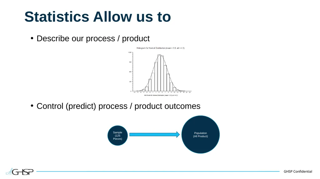
Statistics Allow us to Describe our process / product
Control (predict) process / product outcomes Sample
(125 Pieces) Population
(All Product)<br>
Control (predict) process / product outcomes Sample
(125 Pieces) Population
(All Product)<br>
08
Important Notes Statistical conclusions require useful data
We need to measure the right thing
Determining what data to collect and how to collect it are important steps in the APQP / continuous improvement process
We need to have confidence the data collected is accurate
A good measurement system is required to collect data
Be sure the measurement system analysis (MSA) is acceptable before collecting data
There is a separate training available for MSA
Reduce / Eliminate Waste
Data that doesn’t provide useful information drives waste
We want to gain the most useful information from the least amount of data possible!<br>
09
Types of Data Variable Data (Continuous Data)
Measurements on a continuous scale
Examples
Product Dimensions
Weight
Time
Cost
Process parameters (cutting speed, injection pressure, etc.)
Attribute Data (Discrete Data)
Data by counting
Examples
Count of defective parts from production
Number of chips on a painted part<br>
Measurements on a continuous scale
Examples
Product Dimensions
Weight
Time
Cost
Process parameters (cutting speed, injection pressure, etc.)
Attribute Data (Discrete Data)
Data by counting
Examples
Count of defective parts from production
Number of chips on a painted part<br>
10
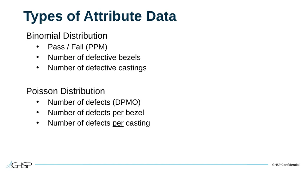
Types of Attribute Data Binomial Distribution
Pass / Fail (PPM)
Number of defective bezels
Number of defective castings
Poisson Distribution
Number of defects (DPMO)
Number of defects per bezel
Number of defects per casting<br>
Pass / Fail (PPM)
Number of defective bezels
Number of defective castings
Poisson Distribution
Number of defects (DPMO)
Number of defects per bezel
Number of defects per casting<br>
11
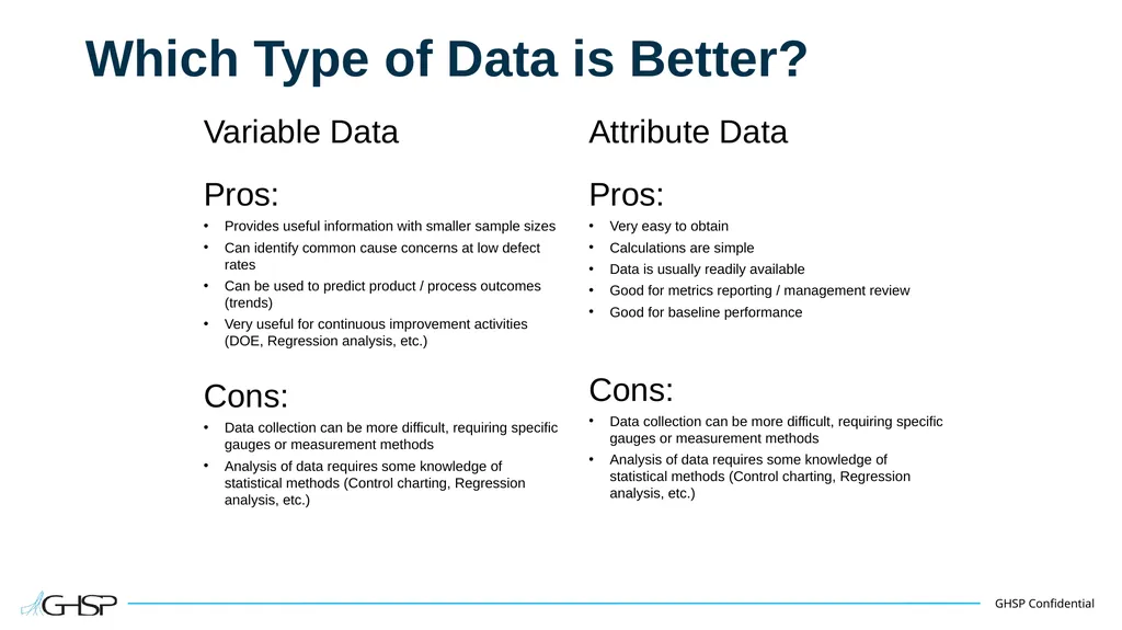
Which Type of Data is Better? Variable Data Pros:
Provides useful information with smaller sample sizes
Can identify common cause concerns at low defect rates
Can be used to predict product / process outcomes (trends)
Very useful for continuous improvement activities (DOE, Regression analysis, etc.)
Cons:
Data collection can be more difficult, requiring specific gauges or measurement methods
Analysis of data requires some knowledge of statistical methods (Control charting, Regression analysis, etc.) Attribute Data Pros:
Very easy to obtain
Calculations are simple
Data is usually readily available
Good for metrics reporting / management review
Good for baseline performance
Cons:
Data collection can be more difficult, requiring specific gauges or measurement methods
Analysis of data requires some knowledge of statistical methods (Control charting, Regression analysis, etc.)<br>
12
Introduction to Statistics Goal:
Define basic statistical tools
Define types of distributions
Understand the Central Limit Theorem
Understand normal distributions<br>
Define basic statistical tools
Define types of distributions
Understand the Central Limit Theorem
Understand normal distributions<br>
13
Definitions Population: A group of all possible objects
Subgroup (Sample): One or more observations used to analyze the performance of a process.
Distribution: A method of describing the output of a stable source of variation, where individual values as a group form a pattern that can be described in terms of its location, spread and shape.<br>
Subgroup (Sample): One or more observations used to analyze the performance of a process.
Distribution: A method of describing the output of a stable source of variation, where individual values as a group form a pattern that can be described in terms of its location, spread and shape.<br>
14
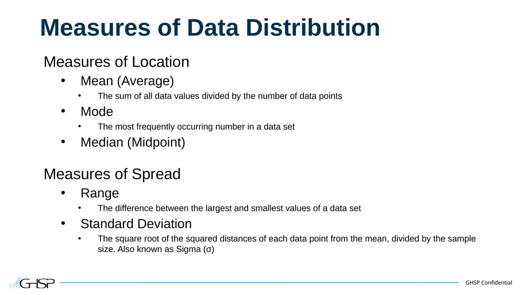
Measures of Data Distribution Measures of Location
Mean (Average)
The sum of all data values divided by the number of data points
Mode
The most frequently occurring number in a data set
Median (Midpoint)
Measures of Spread
Range
The difference between the largest and smallest values of a data set
Standard Deviation
The square root of the squared distances of each data point from the mean, divided by the sample size. Also known as Sigma (σ)<br>
15
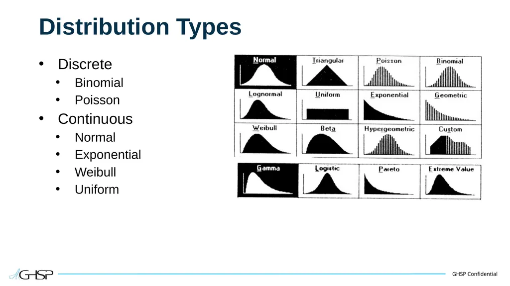
Distribution Types Discrete
Binomial
Poisson
Continuous
Normal
Exponential
Weibull
Uniform<br>
Binomial
Poisson
Continuous
Normal
Exponential
Weibull
Uniform<br>
16
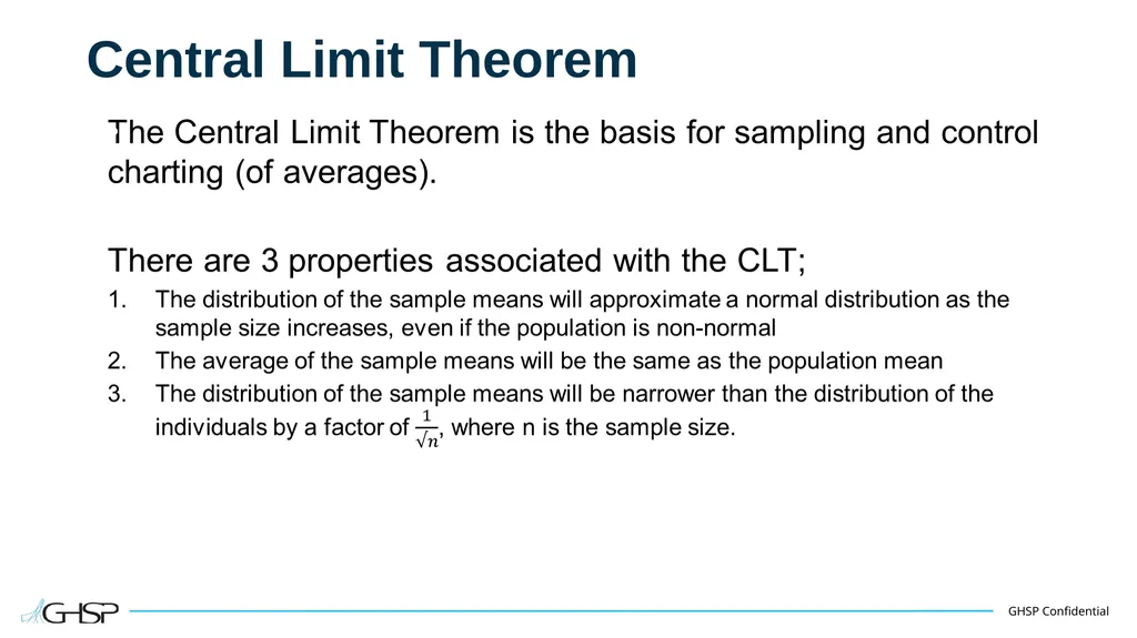
Central Limit Theorem<br>
17
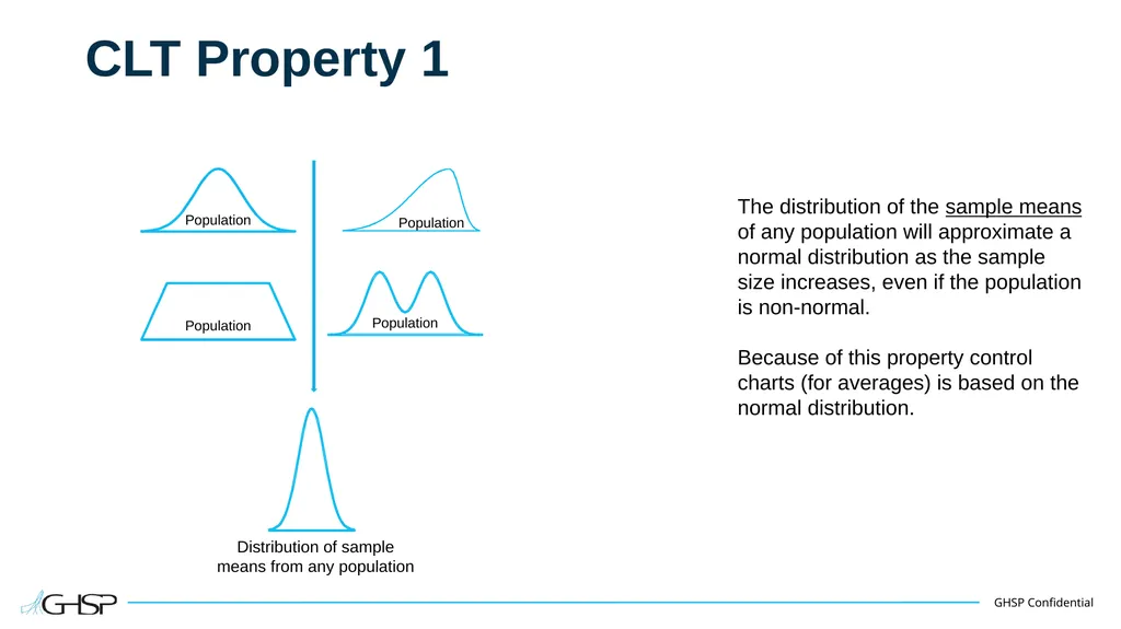
CLT Property 1 The distribution of the sample means of any population will approximate a normal distribution as the sample size increases, even if the population is non-normal.
Because of this property control charts (for averages) is based on the normal distribution. Population Population Population Population Distribution of sample means from any population<br>
Because of this property control charts (for averages) is based on the normal distribution. Population Population Population Population Distribution of sample means from any population<br>
18
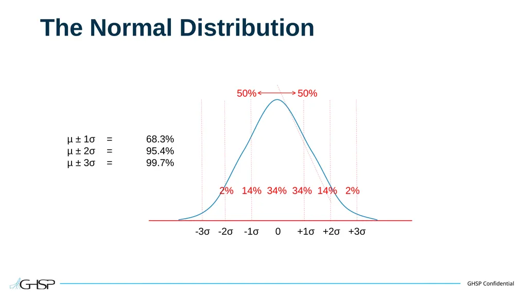
The Normal Distribution µ ± 1σ = 68.3%
µ ± 2σ = 95.4%
µ ± 3σ = 99.7% 2% 14% 34% 34% 14% 2%<br>
µ ± 2σ = 95.4%
µ ± 3σ = 99.7% 2% 14% 34% 34% 14% 2%<br>
19
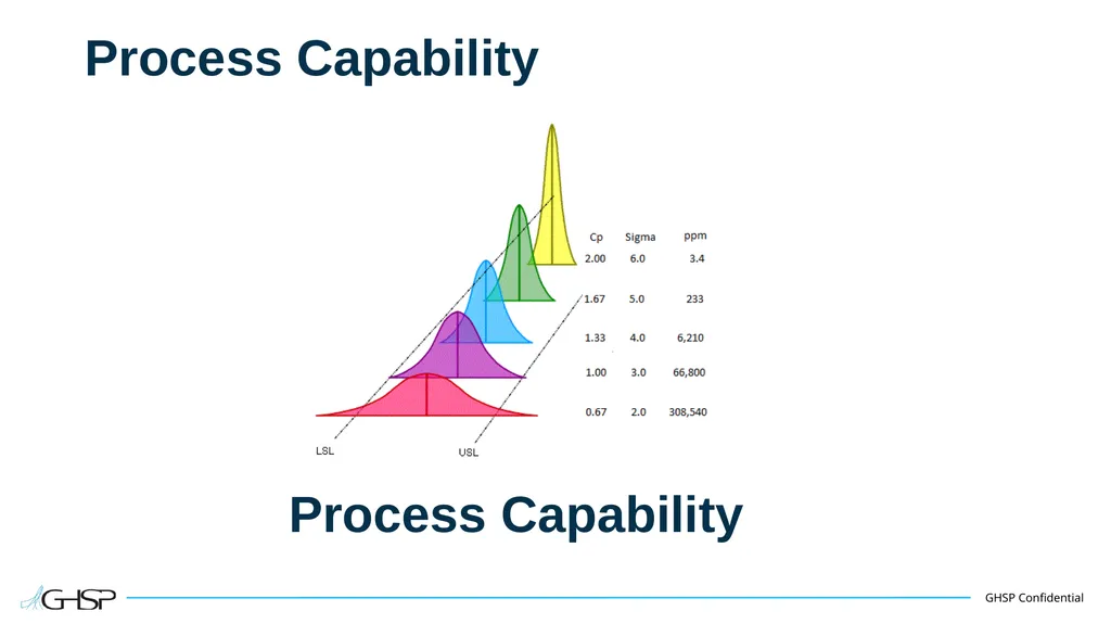
Process Capability Process Capability<br>
20
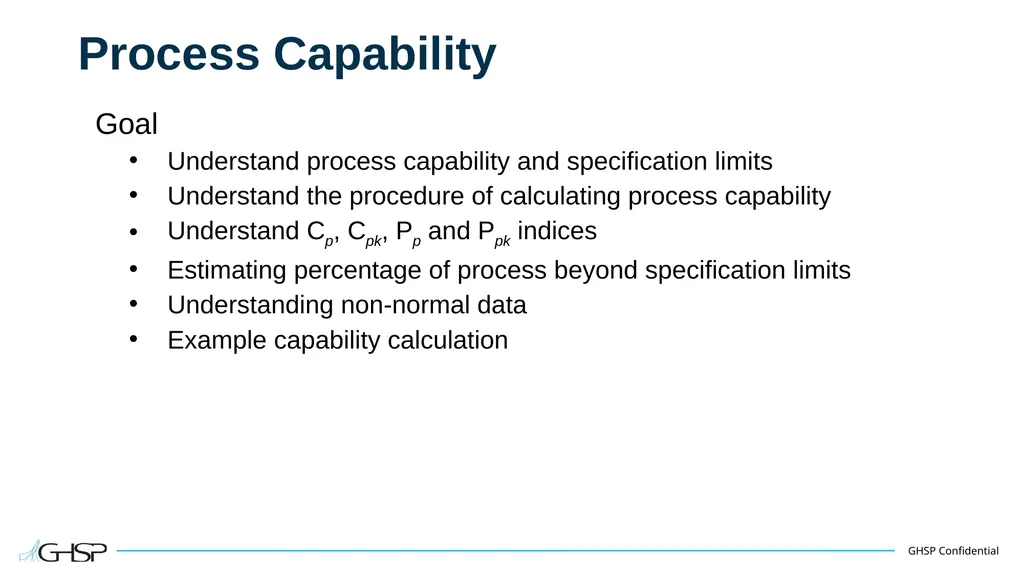
Process Capability Goal
Understand process capability and specification limits
Understand the procedure of calculating process capability
Understand Cp, Cpk, Pp and Ppk indices
Estimating percentage of process beyond specification limits
Understanding non-normal data
Example capability calculation<br>
Understand process capability and specification limits
Understand the procedure of calculating process capability
Understand Cp, Cpk, Pp and Ppk indices
Estimating percentage of process beyond specification limits
Understanding non-normal data
Example capability calculation<br>
21
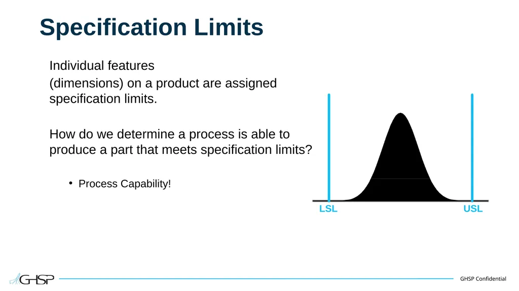
Specification Limits Individual features
(dimensions) on a product are assigned specification limits.
How do we determine a process is able to produce a part that meets specification limits?
Process Capability! LSL USL<br>
(dimensions) on a product are assigned specification limits.
How do we determine a process is able to produce a part that meets specification limits?
Process Capability! LSL USL<br>
22
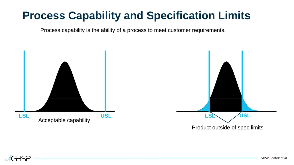
Process Capability and Specification Limits Process capability is the ability of a process to meet customer requirements. LSL USL Acceptable capability LSL USL Product outside of spec limits<br>
23
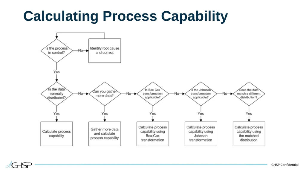
Calculating Process Capability<br>
24
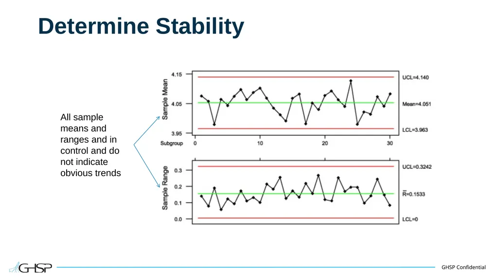
Determine Stability All sample means and ranges and in control and do not indicate obvious trends<br>
25
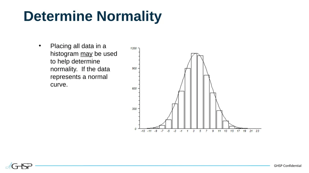
Determine Normality Placing all data in a histogram may be used to help determine normality. If the data represents a normal curve.<br>
26
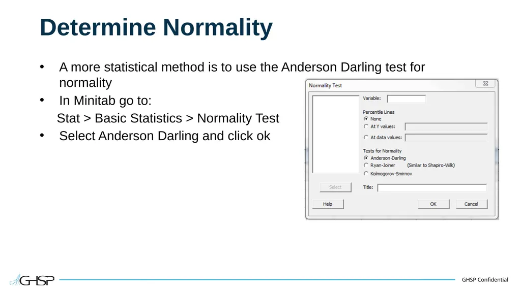
Determine Normality A more statistical method is to use the Anderson Darling test for normality
In Minitab go to:
Stat > Basic Statistics > Normality Test
Select Anderson Darling and click ok<br>
In Minitab go to:
Stat > Basic Statistics > Normality Test
Select Anderson Darling and click ok<br>
27
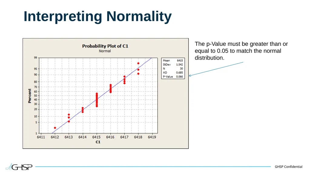
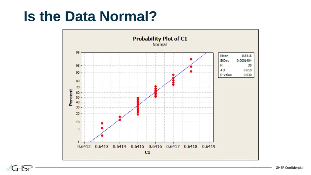
Interpreting Normality The p-Value must be greater than or equal to 0.05 to match the normal distribution.<br>
28
Process Indices Indices of process variation only, in regard to specification;
Cp and Pp
Indices of process variation and centering combined, in regard to specification;
Cpk and Ppk<br>
Cp and Pp
Indices of process variation and centering combined, in regard to specification;
Cpk and Ppk<br>
29
Note Before calculating capability or performance indices we need to make sure of a couple of things!
The process needs to be stable (in control)
The process needs to be normal
A completed MSA needs to prove the measurement system is acceptable
If the above items are not met understand the results of the capability studies may be inaccurate. Also, per the AIAG PPAP manual (4th Edition) if the above items are not met corrective actions may be required prior to PPAP submittal.<br>
30
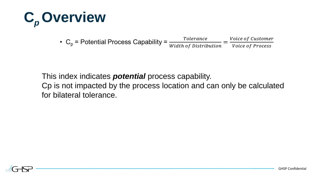
Cp Overview This index indicates potential process capability.
Cp is not impacted by the process location and can only be calculated for bilateral tolerance.<br>
Cp is not impacted by the process location and can only be calculated for bilateral tolerance.<br>
31
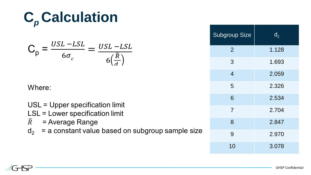
Cp Calculation<br>
32
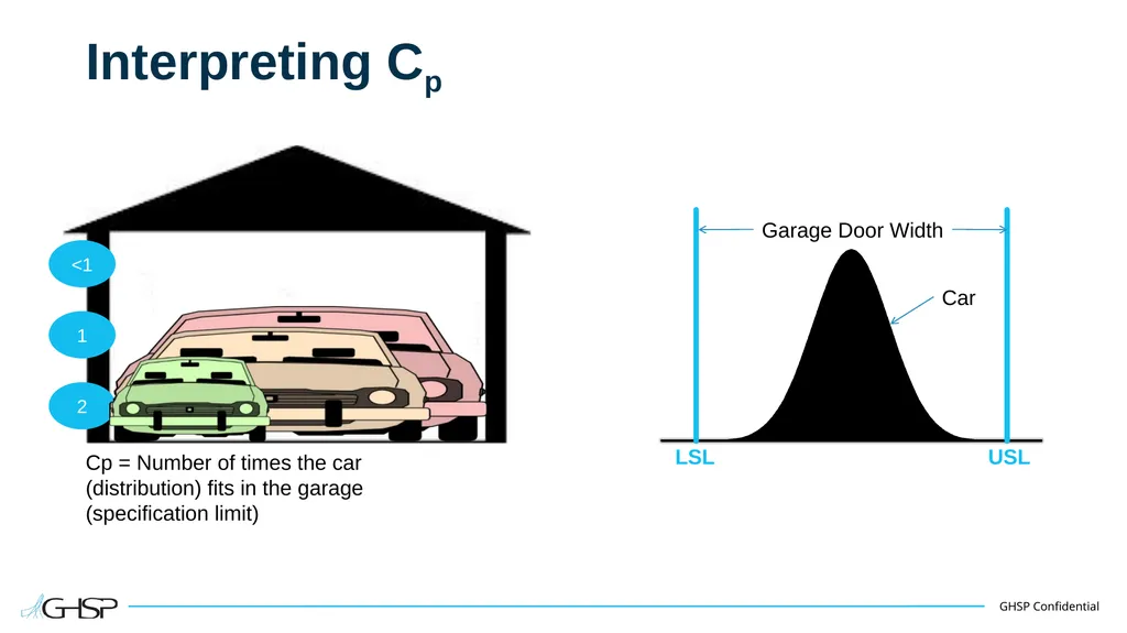
Interpreting Cp <1 1 2 Cp = Number of times the car (distribution) fits in the garage (specification limit) LSL USL Garage Door Width Car<br>
33
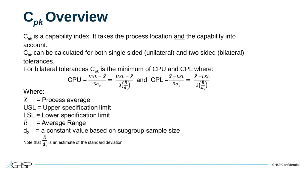
Cpk Overview Cpk is a capability index. It takes the process location and the capability into account.
Cpk can be calculated for both single sided (unilateral) and two sided (bilateral) tolerances.
For bilateral tolerances Cpk is the minimum of CPU and CPL where:<br>
Cpk can be calculated for both single sided (unilateral) and two sided (bilateral) tolerances.
For bilateral tolerances Cpk is the minimum of CPU and CPL where:<br>
34
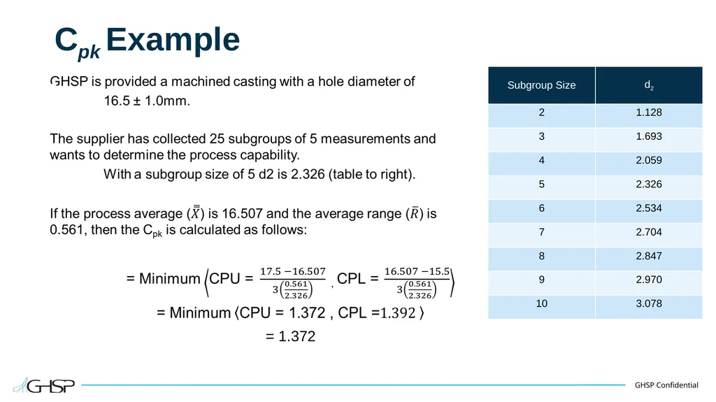
Cpk Example = 1.372<br>
35
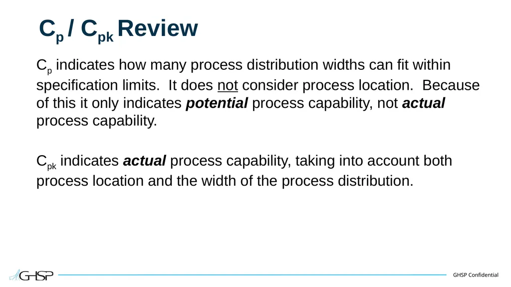
Cp / Cpk Review Cp indicates how many process distribution widths can fit within specification limits. It does not consider process location. Because of this it only indicates potential process capability, not actual process capability.
Cpk indicates actual process capability, taking into account both process location and the width of the process distribution.<br>
Cpk indicates actual process capability, taking into account both process location and the width of the process distribution.<br>
36
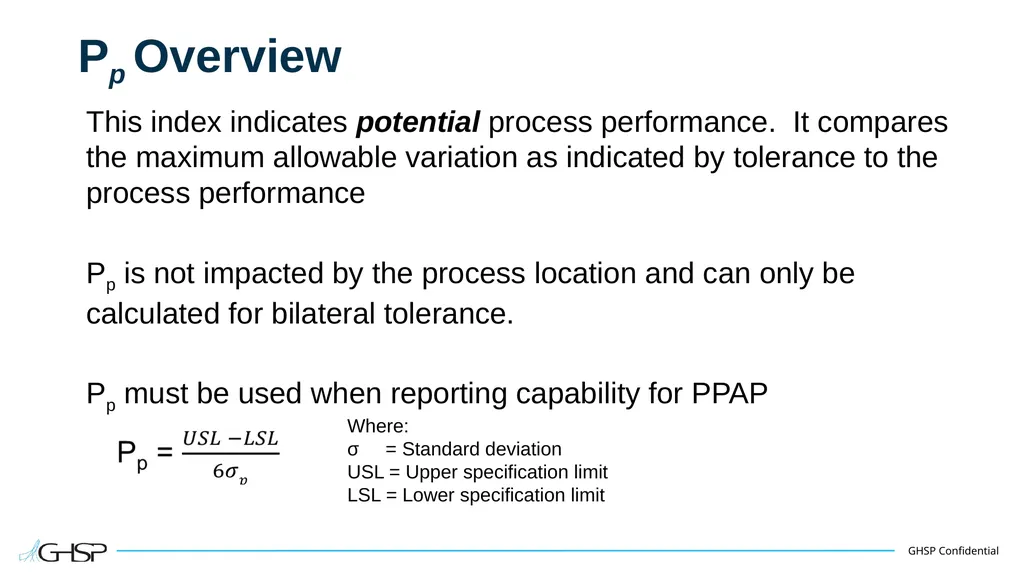
Pp Overview This index indicates potential process performance. It compares the maximum allowable variation as indicated by tolerance to the process performance
Pp is not impacted by the process location and can only be calculated for bilateral tolerance.
Pp must be used when reporting capability for PPAP Where:
σ = Standard deviation
USL = Upper specification limit
LSL = Lower specification limit<br>
Pp is not impacted by the process location and can only be calculated for bilateral tolerance.
Pp must be used when reporting capability for PPAP Where:
σ = Standard deviation
USL = Upper specification limit
LSL = Lower specification limit<br>
37
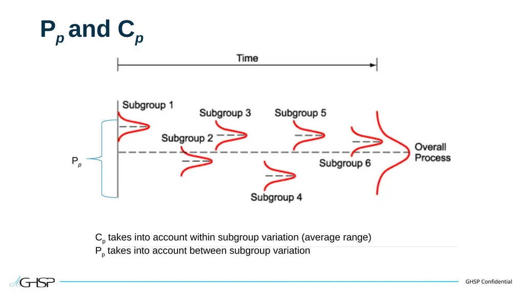
Pp and Cp Pp Cp takes into account within subgroup variation (average range)
Pp takes into account between subgroup variation<br>
Pp takes into account between subgroup variation<br>
38
Ppk Overview Ppk is a performance index. It indicates actual process performance, taking into account both process location and overall process variation.
Ppk shows if a process is actually meeting customer requirements.
Ppk can be used for both unilateral and bilateral tolerances.
Ppk must be used when reporting capability for PPAP<br>
Ppk shows if a process is actually meeting customer requirements.
Ppk can be used for both unilateral and bilateral tolerances.
Ppk must be used when reporting capability for PPAP<br>
39
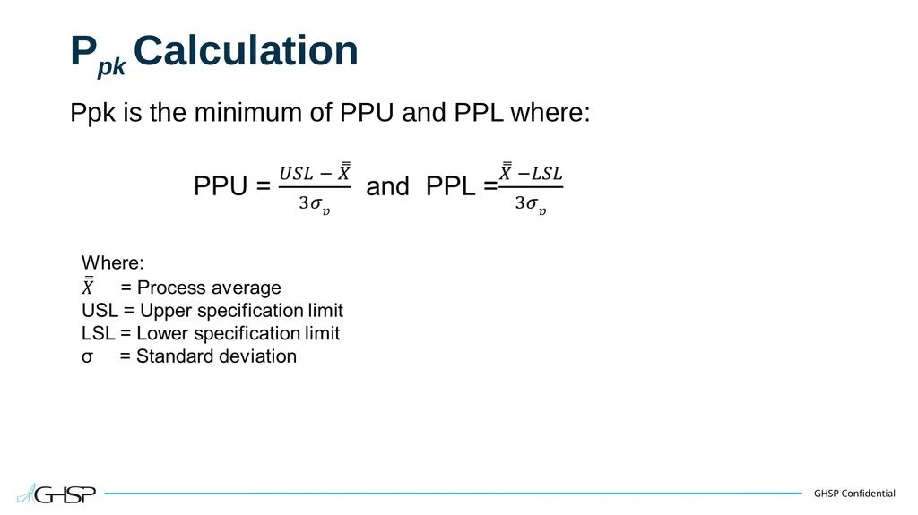
Ppk Calculation Ppk is the minimum of PPU and PPL where:<br>
40
Pp / Ppk Review Pp indicates how many process distribution widths can fit within specification limits. It does not consider process location. Because of this it only indicates potential process performance, not actual process performance.
Ppk indicates actual process performance, taking into account both process location and the width of the process distribution.<br>
Ppk indicates actual process performance, taking into account both process location and the width of the process distribution.<br>
41
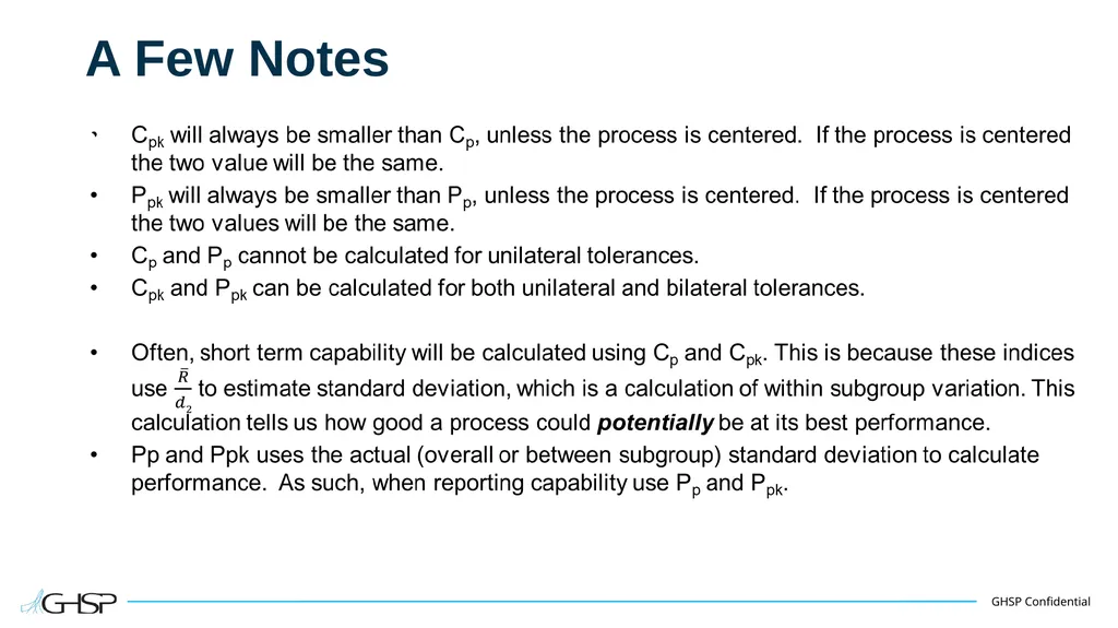
A Few Notes<br>
42
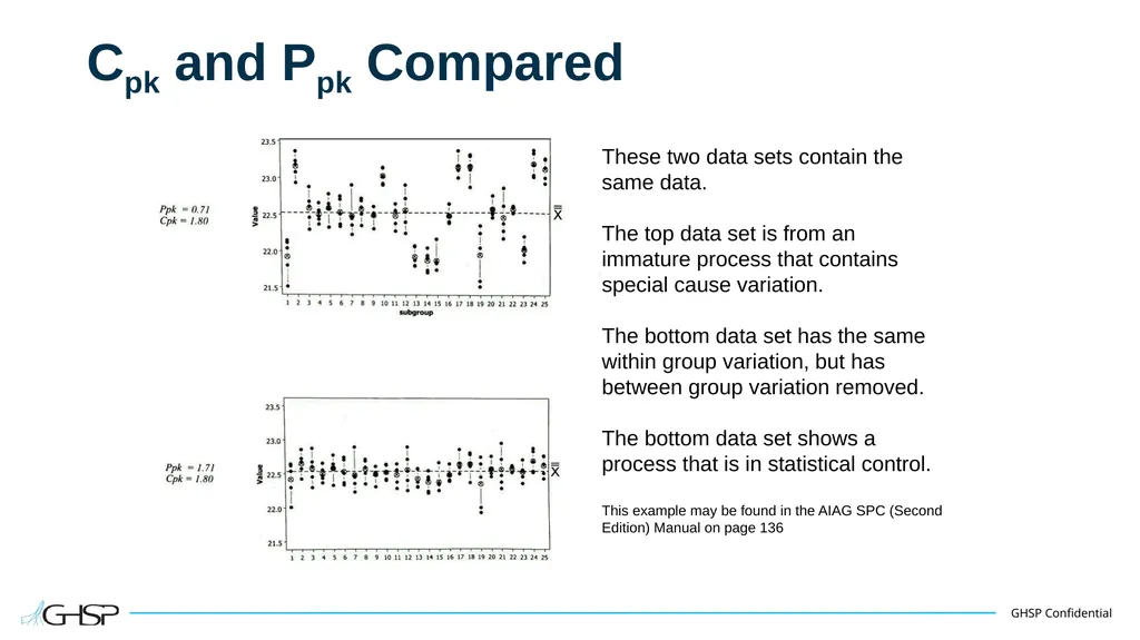
Cpk and Ppk Compared These two data sets contain the same data.
The top data set is from an immature process that contains special cause variation.
The bottom data set has the same within group variation, but has between group variation removed.
The bottom data set shows a process that is in statistical control.
This example may be found in the AIAG SPC (Second Edition) Manual on page 136<br>
43
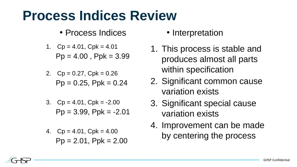
Process Indices Review Process Indices Cp = 4.01, Cpk = 4.01
Pp = 4.00 , Ppk = 3.99
Cp = 0.27, Cpk = 0.26
Pp = 0.25, Ppk = 0.24
Cp = 4.01, Cpk = -2.00
Pp = 3.99, Ppk = -2.01
Cp = 4.01, Cpk = 4.00
Pp = 2.01, Ppk = 2.00 Interpretation This process is stable and produces almost all parts within specification
Significant common cause variation exists
Significant special cause variation exists
Improvement can be made by centering the process<br>
44
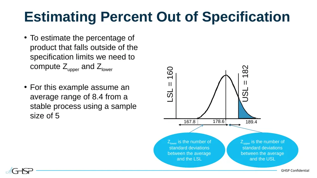
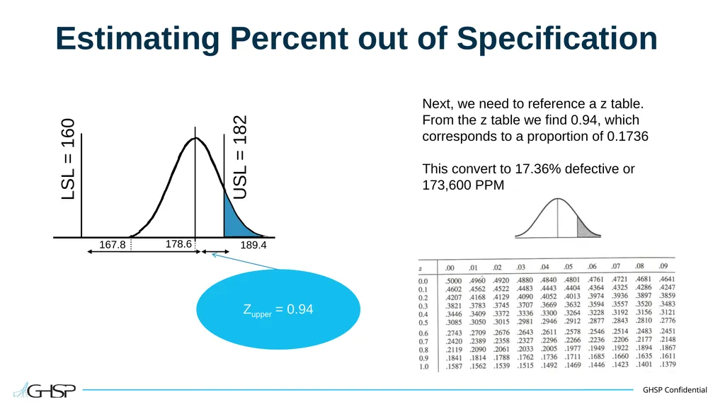
Estimating Percent Out of Specification To estimate the percentage of product that falls outside of the specification limits we need to compute Zupper and Zlower
For this example assume an average range of 8.4 from a stable process using a sample size of 5 USL = 182 LSL = 160 Zupper is the number of standard deviations between the average and the USL Zlower is the number of standard deviations between the average and the LSL 189.4 178.6 167.8<br>
For this example assume an average range of 8.4 from a stable process using a sample size of 5 USL = 182 LSL = 160 Zupper is the number of standard deviations between the average and the USL Zlower is the number of standard deviations between the average and the LSL 189.4 178.6 167.8<br>
45
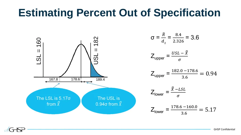
Estimating Percent Out of Specification USL = 182 LSL = 160 189.4 178.6 167.8<br>
46
Estimating Percent out of Specification USL = 182 LSL = 160 Zupper = 0.94 189.4 178.6 167.8 Next, we need to reference a z table.
From the z table we find 0.94, which corresponds to a proportion of 0.1736
This convert to 17.36% defective or 173,600 PPM<br>
From the z table we find 0.94, which corresponds to a proportion of 0.1736
This convert to 17.36% defective or 173,600 PPM<br>
47
Understanding Non-Normal Data What happens when data used for capability is not normally distributed?
Cp and Pp indices are robust in their accuracy with regards to non-normal data.
Cpk and Ppk indices are not robust with regards to non-normal data.
Calculating (and making decisions based on) Ppk and Cpk indices assuming normality with non-normal data can be misleading.<br>
Cp and Pp indices are robust in their accuracy with regards to non-normal data.
Cpk and Ppk indices are not robust with regards to non-normal data.
Calculating (and making decisions based on) Ppk and Cpk indices assuming normality with non-normal data can be misleading.<br>
48
Understanding Non-Normal Data What do I do if my data is not normal?
Gather more data
This may or may not be an option given timing and cost.
The Central Limit Theorem (covered earlier) states that all population means resemble the normal distribution with larger sample size
Transform the data
Using either the Box-Cox or Johnson transformations we can transform non-normal data to a near normal form
This allows use to accurately calculate Cpk and Ppk indices and the proportion nonconforming
Calculate capabilities based on different distributions<br>
49
Box-Cox Transformation<br>
50
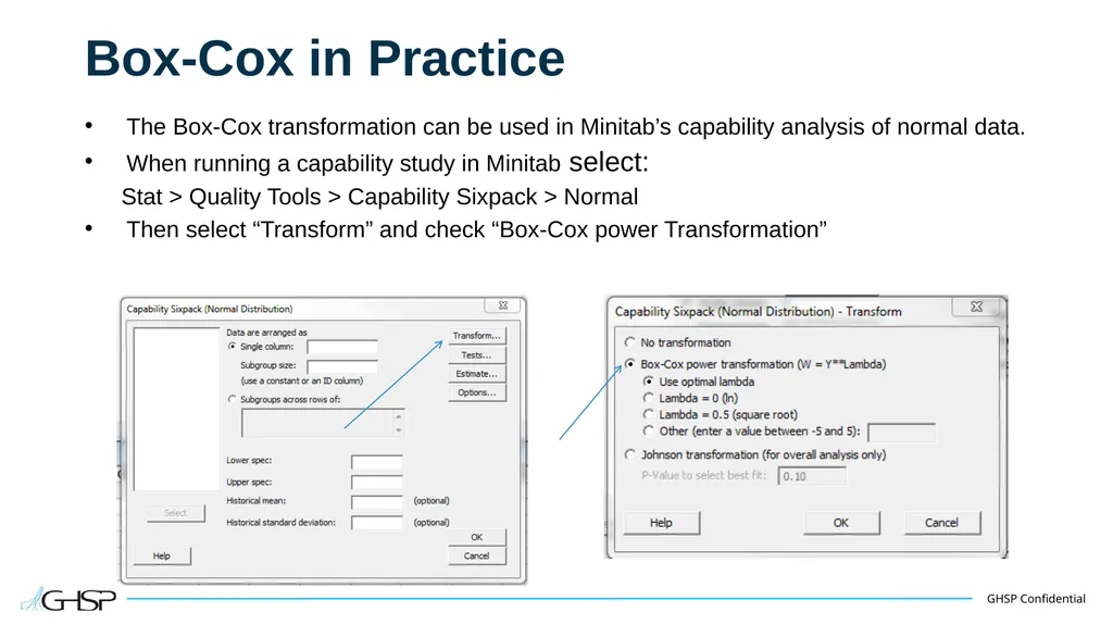
Box-Cox in Practice The Box-Cox transformation can be used in Minitab’s capability analysis of normal data.
When running a capability study in Minitab select:
Stat > Quality Tools > Capability Sixpack > Normal
Then select “Transform” and check “Box-Cox power Transformation”<br>
When running a capability study in Minitab select:
Stat > Quality Tools > Capability Sixpack > Normal
Then select “Transform” and check “Box-Cox power Transformation”<br>
51
Johnson Transformation The Johnson Transformation uses a system of transformations that yield approximate normality.
The Johnson Transformation covers:
Bounded data
Log normal data
Unbounded data
This system of transformations cover all possible unimodal distribution forms (skewness-kurtosis)
This transformation can also be ran in Minitab<br>
The Johnson Transformation covers:
Bounded data
Log normal data
Unbounded data
This system of transformations cover all possible unimodal distribution forms (skewness-kurtosis)
This transformation can also be ran in Minitab<br>
52
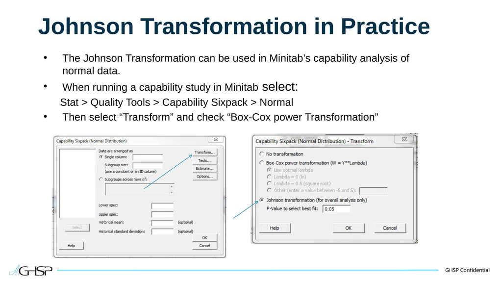
Johnson Transformation in Practice The Johnson Transformation can be used in Minitab’s capability analysis of normal data.
When running a capability study in Minitab select:
Stat > Quality Tools > Capability Sixpack > Normal
Then select “Transform” and check “Box-Cox power Transformation”<br>
When running a capability study in Minitab select:
Stat > Quality Tools > Capability Sixpack > Normal
Then select “Transform” and check “Box-Cox power Transformation”<br>
53
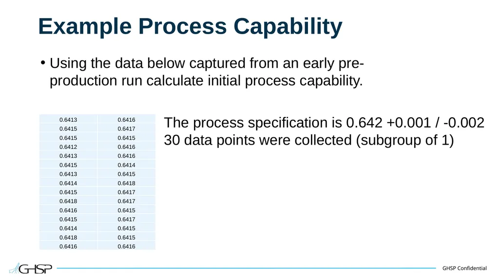
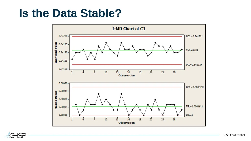
Example Process Capability Using the data below captured from an early pre-production run calculate initial process capability. The process specification is 0.642 +0.001 / -0.002
30 data points were collected (subgroup of 1)<br>
30 data points were collected (subgroup of 1)<br>
54
Is the Data Stable?<br>
55
Is the Data Normal?<br>
56
Calculate Capability<br>
57
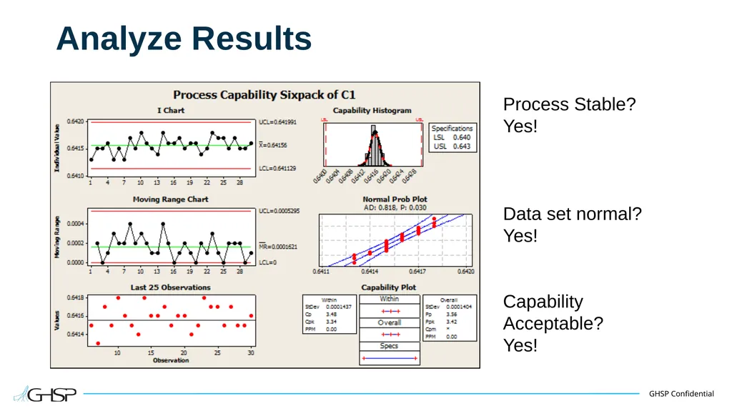
Analyze Results Process Stable?
Yes!
Data set normal?
Yes!
Capability Acceptable?
Yes!<br>
Yes!
Data set normal?
Yes!
Capability Acceptable?
Yes!<br>
58
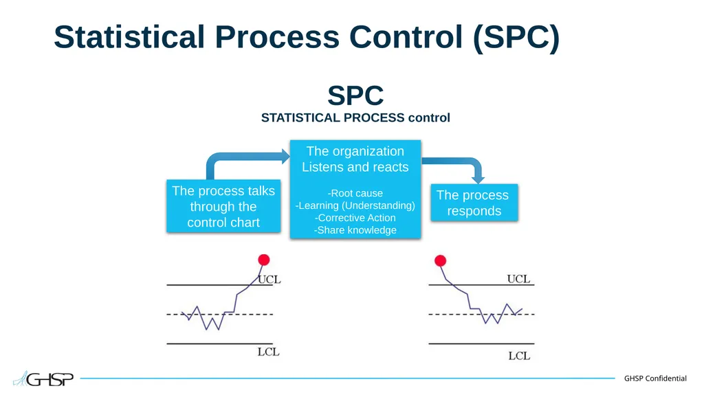
Statistical Process Control (SPC) SPC
STATISTICAL PROCESS control The process talks
through the
control chart The process
responds The organization
Listens and reacts
-Root cause
-Learning (Understanding)
-Corrective Action
-Share knowledge<br>
through the
control chart The process
responds The organization
Listens and reacts
-Root cause
-Learning (Understanding)
-Corrective Action
-Share knowledge<br>
59
Why do we need process control? Why prevention instead of detection?
Detection tolerates waste, Prevention avoids it.<br>
Detection tolerates waste, Prevention avoids it.<br>
60
Variation There are two types of variation
Common Cause
The many factors that result in variation that is consistently acting on a process. If only common causes are present in a process it is considered stable and in control. If only common cause variation is present in a process the process outcome is predictable.
Special Cause
Also known as assignable causes, special causes are factors that result in variation that only affect some of the process output. Special cause variation results in one or more points outside of controls limits and / or non-random patterns of points within control limits. Special cause variation is not predictable and, if present in a process, results in instability and out of control conditions.<br>
61
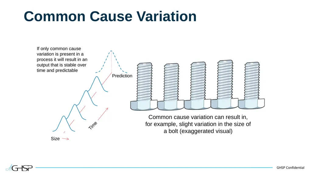
Common Cause Variation Common cause variation can result in, for example, slight variation in the size of a bolt (exaggerated visual) If only common cause variation is present in a process it will result in an output that is stable over time and predictable<br>