
Stream Codes for Data Compression Yehong, Wang
SN
Published · 71 slides · 0 views
1 / 1

Description
Stream Codes for Data Compression Yehong, Wang Wei, Wang Sheng, Jinyang, Gordon Outline Introduction Overview of Huffman Coding Arithmetic Coding Encoding and Decoding Probabilistic Model (break) Loss Analysis Lempel-Ziv Coding Summary Why
Related Topics
Share
Embed code
Download this presentation From Below
"Stream Codes for Data Compression Yehong, Wang" is the property of its rightful owner. Permission is granted to download and print the materials on this website for personal, non-commercial use only, and to display it on your personal computer provided you do not modify the materials and that you retain all copyright notices contained in the materials. By downloading content from our website, you accept the terms of this agreement.
Presentation Transcript
01
Stream Codes
for Data Compression Yehong, Wang Wei, Wang Sheng, Jinyang, Gordon<br>
02
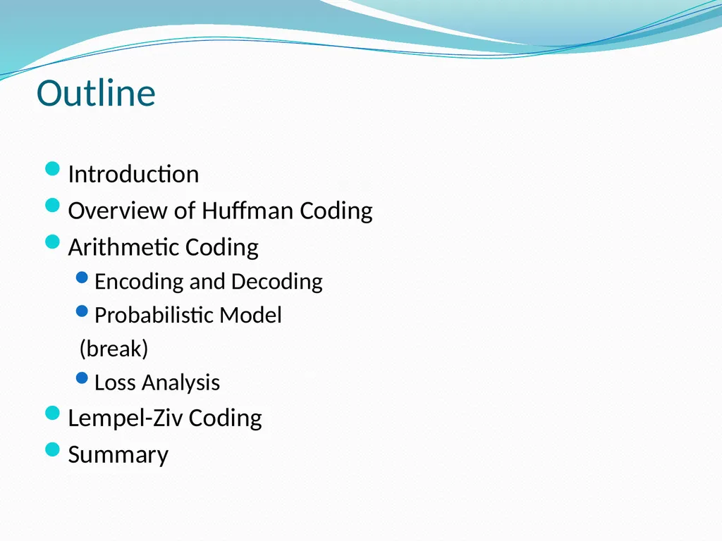
Outline Introduction
Overview of Huffman Coding
Arithmetic Coding
Encoding and Decoding
Probabilistic Model
(break)
Loss Analysis
Lempel-Ziv Coding
Summary<br>
Overview of Huffman Coding
Arithmetic Coding
Encoding and Decoding
Probabilistic Model
(break)
Loss Analysis
Lempel-Ziv Coding
Summary<br>
03
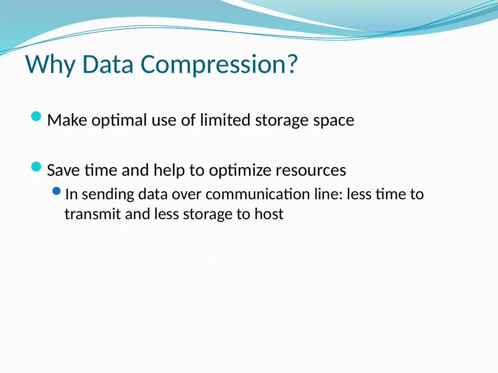
Why Data Compression? Make optimal use of limited storage space
Save time and help to optimize resources
In sending data over communication line: less time to transmit and less storage to host<br>
Save time and help to optimize resources
In sending data over communication line: less time to transmit and less storage to host<br>
04
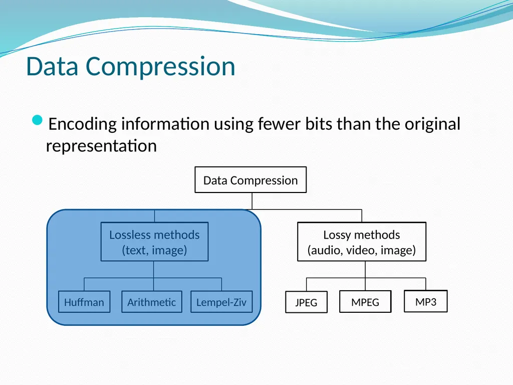
Data Compression Encoding information using fewer bits than the original representation<br>
05
Outline Introduction
Overview of Huffman Coding
Arithmetic Coding
Encoding and Decoding
Probabilistic Model
(break)
Loss Analysis
Lempel-Ziv Coding
Summary<br>
Overview of Huffman Coding
Arithmetic Coding
Encoding and Decoding
Probabilistic Model
(break)
Loss Analysis
Lempel-Ziv Coding
Summary<br>
06
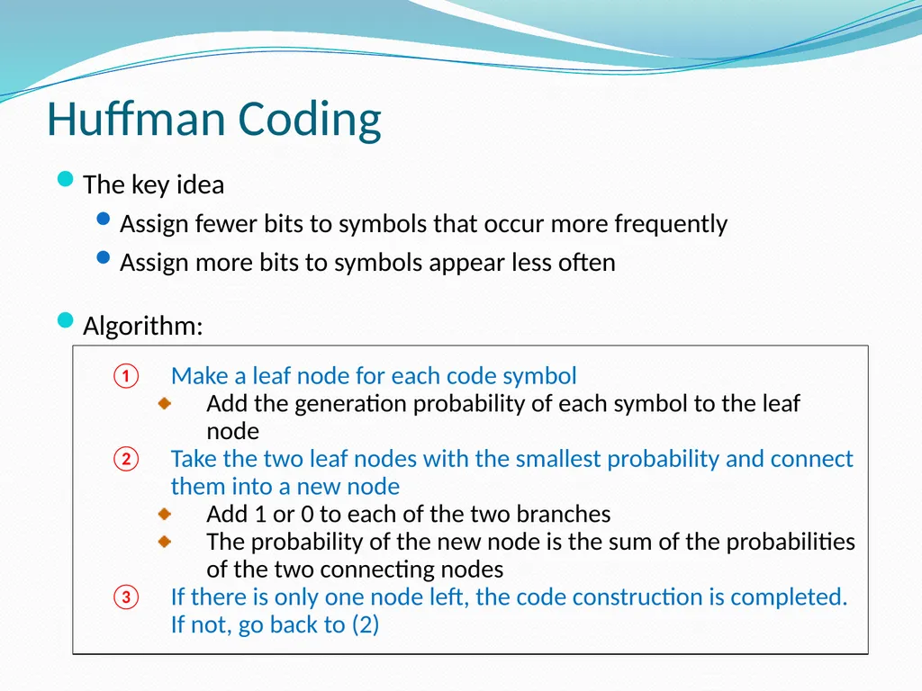
Huffman Coding The key idea
Assign fewer bits to symbols that occur more frequently
Assign more bits to symbols appear less often
Algorithm: Make a leaf node for each code symbol
Add the generation probability of each symbol to the leaf node
Take the two leaf nodes with the smallest probability and connect them into a new node
Add 1 or 0 to each of the two branches
The probability of the new node is the sum of the probabilities of the two connecting nodes
If there is only one node left, the code construction is completed. If not, go back to (2)<br>
Assign fewer bits to symbols that occur more frequently
Assign more bits to symbols appear less often
Algorithm: Make a leaf node for each code symbol
Add the generation probability of each symbol to the leaf node
Take the two leaf nodes with the smallest probability and connect them into a new node
Add 1 or 0 to each of the two branches
The probability of the new node is the sum of the probabilities of the two connecting nodes
If there is only one node left, the code construction is completed. If not, go back to (2)<br>
07
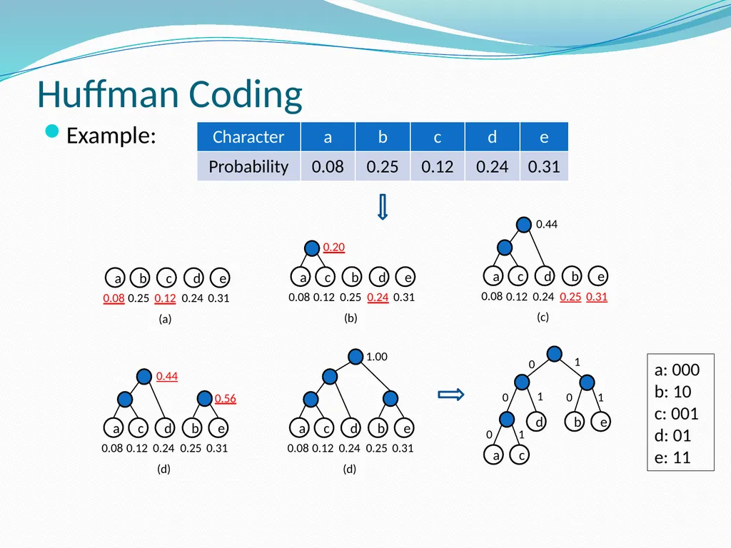
Huffman Coding Example: a: 000
b: 10
c: 001
d: 01
e: 11<br>
b: 10
c: 001
d: 01
e: 11<br>
08
Huffman Coding For an ensemble, the Huffman algorithm produces an optimal symbol code<br>
09
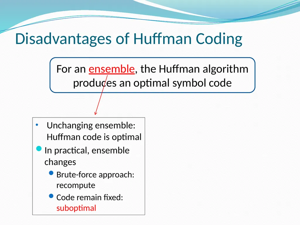
Disadvantages of Huffman Coding For an ensemble, the Huffman algorithm produces an optimal symbol code Unchanging ensemble: Huffman code is optimal
In practical, ensemble changes
Brute-force approach: recompute
Code remain fixed: suboptimal<br>
In practical, ensemble changes
Brute-force approach: recompute
Code remain fixed: suboptimal<br>
10
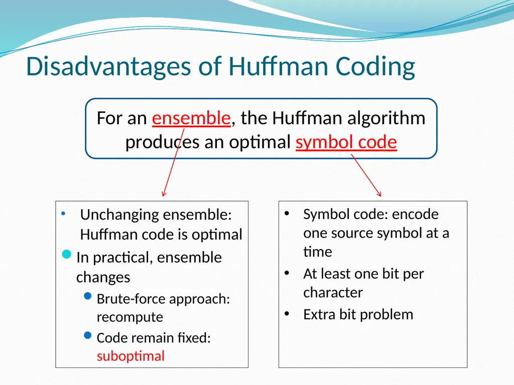
Disadvantages of Huffman Coding For an ensemble, the Huffman algorithm produces an optimal symbol code Unchanging ensemble: Huffman code is optimal
In practical, ensemble changes
Brute-force approach: recompute
Code remain fixed: suboptimal Symbol code: encode one source symbol at a time
At least one bit per character
Extra bit problem<br>
In practical, ensemble changes
Brute-force approach: recompute
Code remain fixed: suboptimal Symbol code: encode one source symbol at a time
At least one bit per character
Extra bit problem<br>
11
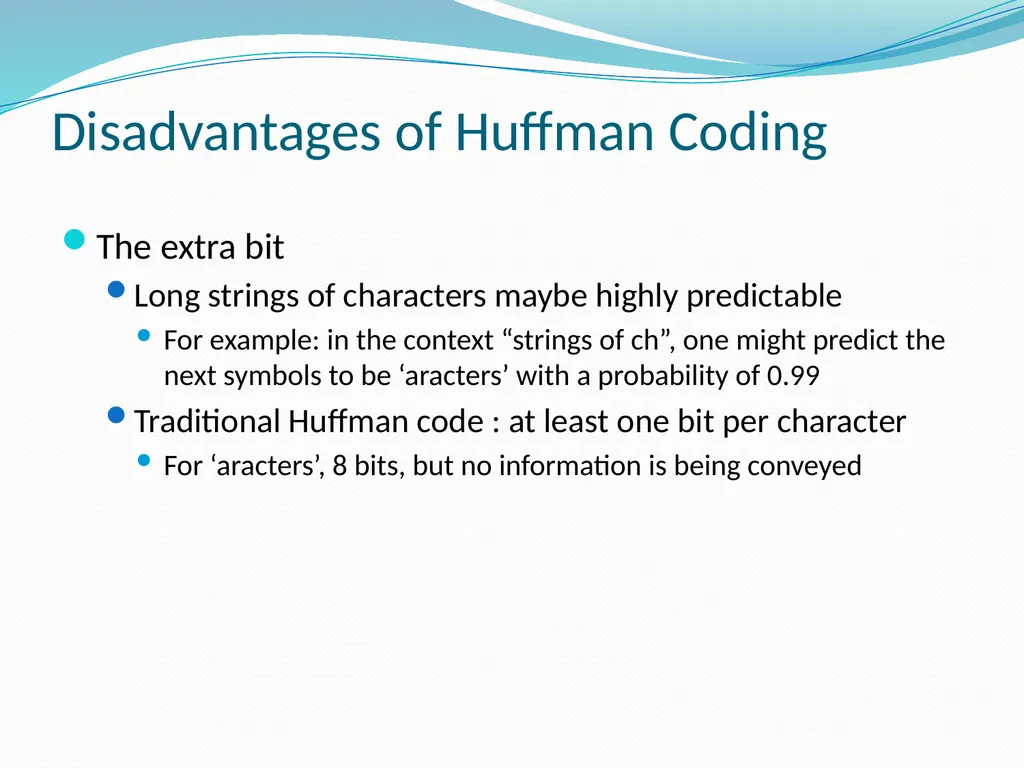
Disadvantages of Huffman Coding The extra bit
Long strings of characters maybe highly predictable
For example: in the context “strings of ch”, one might predict the next symbols to be ‘aracters’ with a probability of 0.99
Traditional Huffman code : at least one bit per character
For ‘aracters’, 8 bits, but no information is being conveyed<br>
Long strings of characters maybe highly predictable
For example: in the context “strings of ch”, one might predict the next symbols to be ‘aracters’ with a probability of 0.99
Traditional Huffman code : at least one bit per character
For ‘aracters’, 8 bits, but no information is being conveyed<br>
12
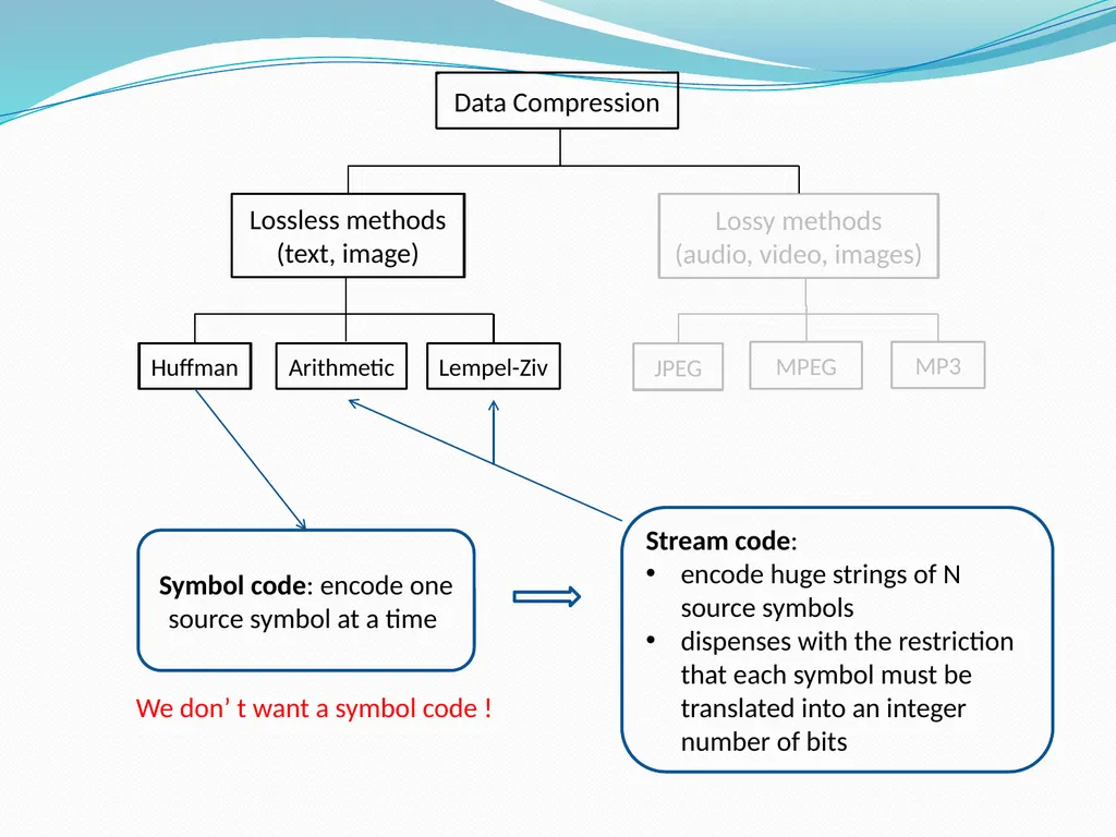
Symbol code: encode one source symbol at a time Stream code:
encode huge strings of N source symbols
dispenses with the restriction that each symbol must be translated into an integer number of bits We don’ t want a symbol code !<br>
encode huge strings of N source symbols
dispenses with the restriction that each symbol must be translated into an integer number of bits We don’ t want a symbol code !<br>
13
Outline Introduction
Overview of Huffman Coding
Arithmetic Coding
Encoding and Decoding
Probabilistic Model
(break)
Loss Analysis
Lempel-Ziv Coding
Summary<br>
Overview of Huffman Coding
Arithmetic Coding
Encoding and Decoding
Probabilistic Model
(break)
Loss Analysis
Lempel-Ziv Coding
Summary<br>
14
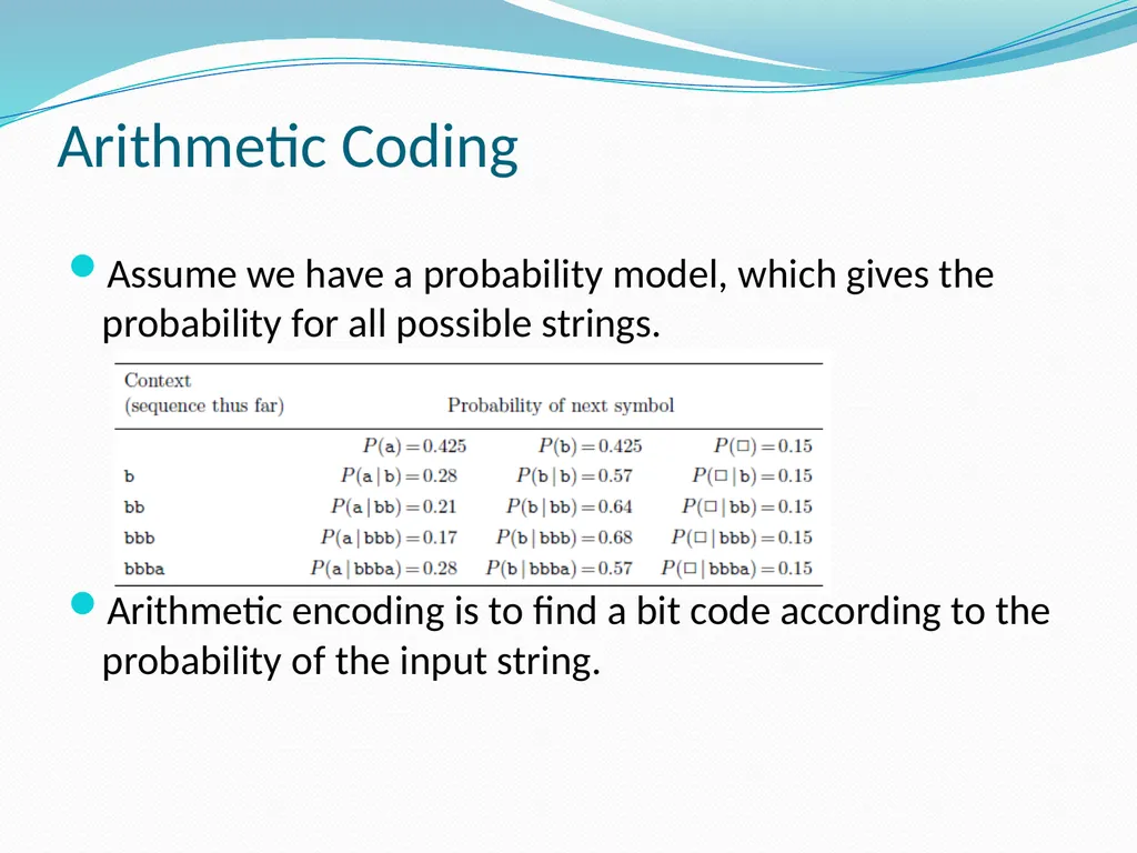
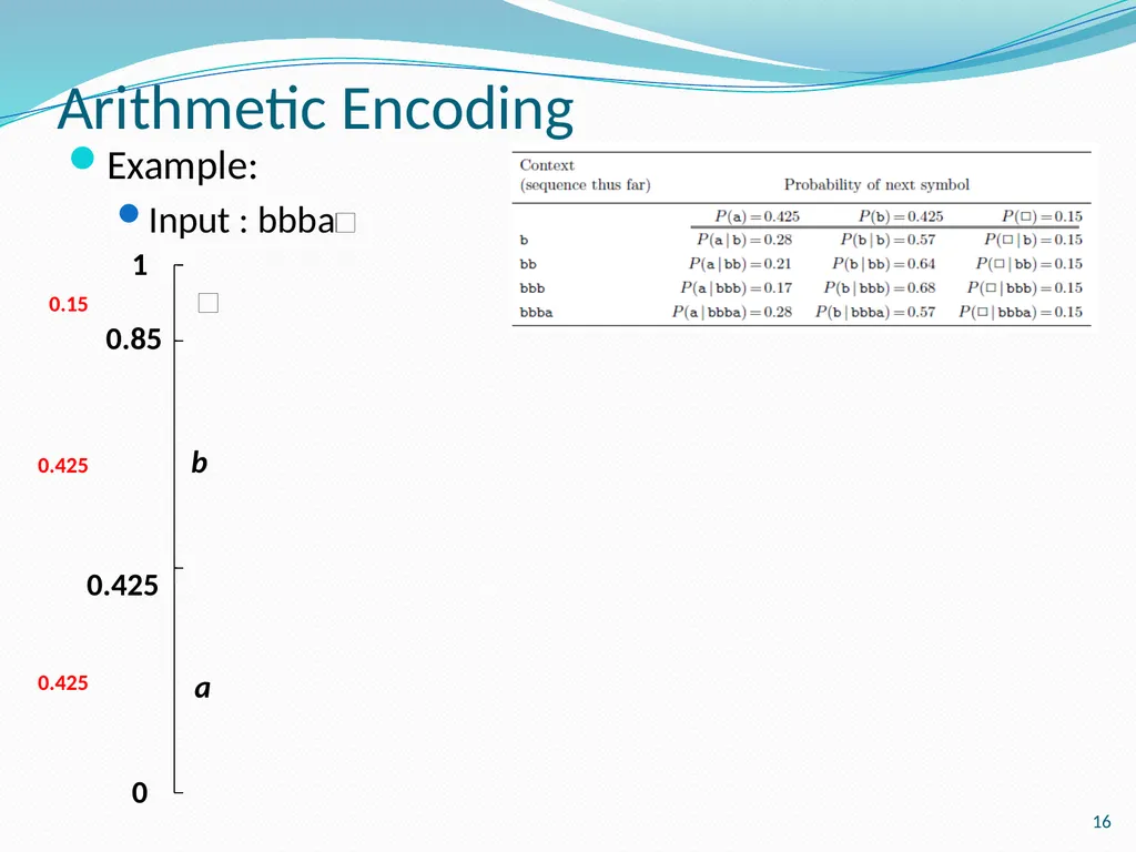
Arithmetic Coding Assume we have a probability model, which gives the probability for all possible strings.
Arithmetic encoding is to find a bit code according to the probability of the input string.<br>
Arithmetic encoding is to find a bit code according to the probability of the input string.<br>
15
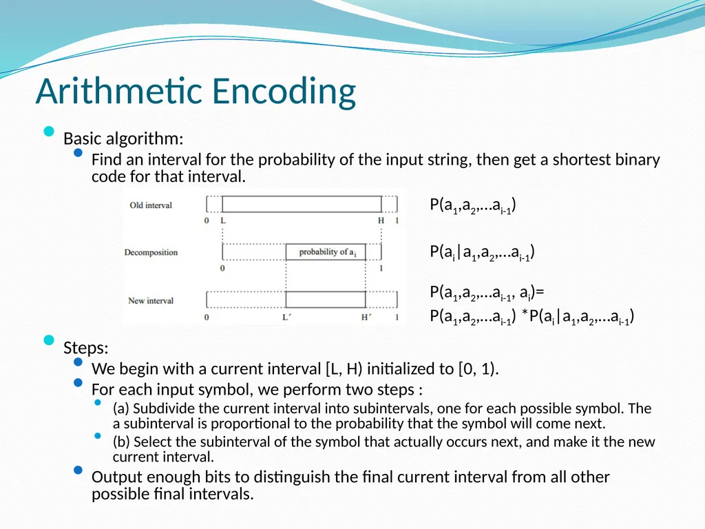
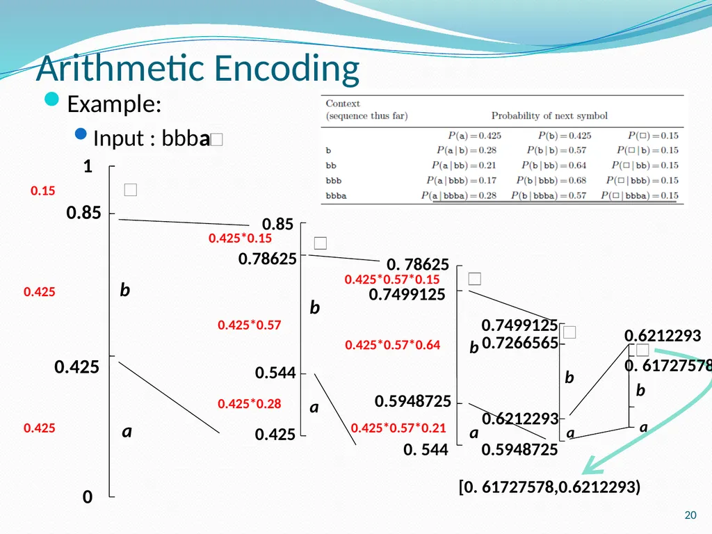
Arithmetic Encoding Basic algorithm:
Find an interval for the probability of the input string, then get a shortest binary code for that interval.
Steps:
We begin with a current interval [L, H) initialized to [0, 1).
For each input symbol, we perform two steps :
(a) Subdivide the current interval into subintervals, one for each possible symbol. The a subinterval is proportional to the probability that the symbol will come next.
(b) Select the subinterval of the symbol that actually occurs next, and make it the new current interval.
Output enough bits to distinguish the final current interval from all other possible final intervals. P(ai|a1,a2,…ai-1) P(a1,a2,…ai-1, ai)=
P(a1,a2,…ai-1) *P(ai|a1,a2,…ai-1) P(a1,a2,…ai-1)<br>
Find an interval for the probability of the input string, then get a shortest binary code for that interval.
Steps:
We begin with a current interval [L, H) initialized to [0, 1).
For each input symbol, we perform two steps :
(a) Subdivide the current interval into subintervals, one for each possible symbol. The a subinterval is proportional to the probability that the symbol will come next.
(b) Select the subinterval of the symbol that actually occurs next, and make it the new current interval.
Output enough bits to distinguish the final current interval from all other possible final intervals. P(ai|a1,a2,…ai-1) P(a1,a2,…ai-1, ai)=
P(a1,a2,…ai-1) *P(ai|a1,a2,…ai-1) P(a1,a2,…ai-1)<br>
16
Arithmetic Encoding Example:
Input : bbba 16 0 1 0.425 0.85 a 0.425 0.15 0.425 b<br>
Input : bbba 16 0 1 0.425 0.85 a 0.425 0.15 0.425 b<br>
17
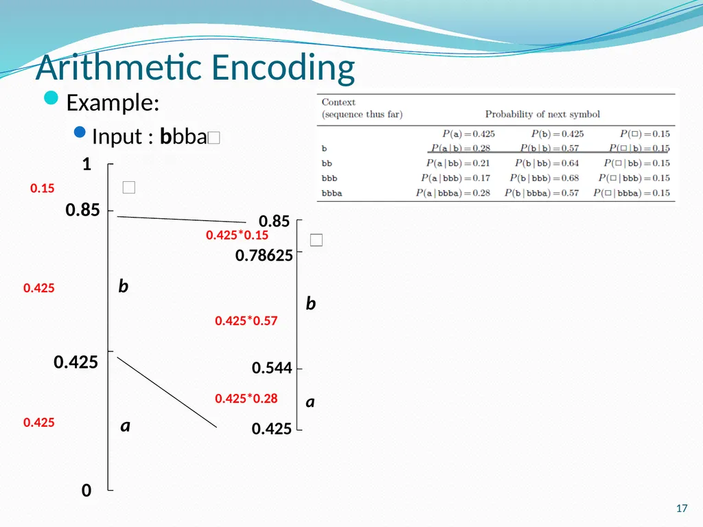
Arithmetic Encoding Example:
Input : bbba 17 0 1 0.425 0.85 a 0.425 0.15 0.425 0.85 0.425 0.544 0.78625 0.425*0.15 0.425*0.57 0.425*0.28 b b a<br>
Input : bbba 17 0 1 0.425 0.85 a 0.425 0.15 0.425 0.85 0.425 0.544 0.78625 0.425*0.15 0.425*0.57 0.425*0.28 b b a<br>
18
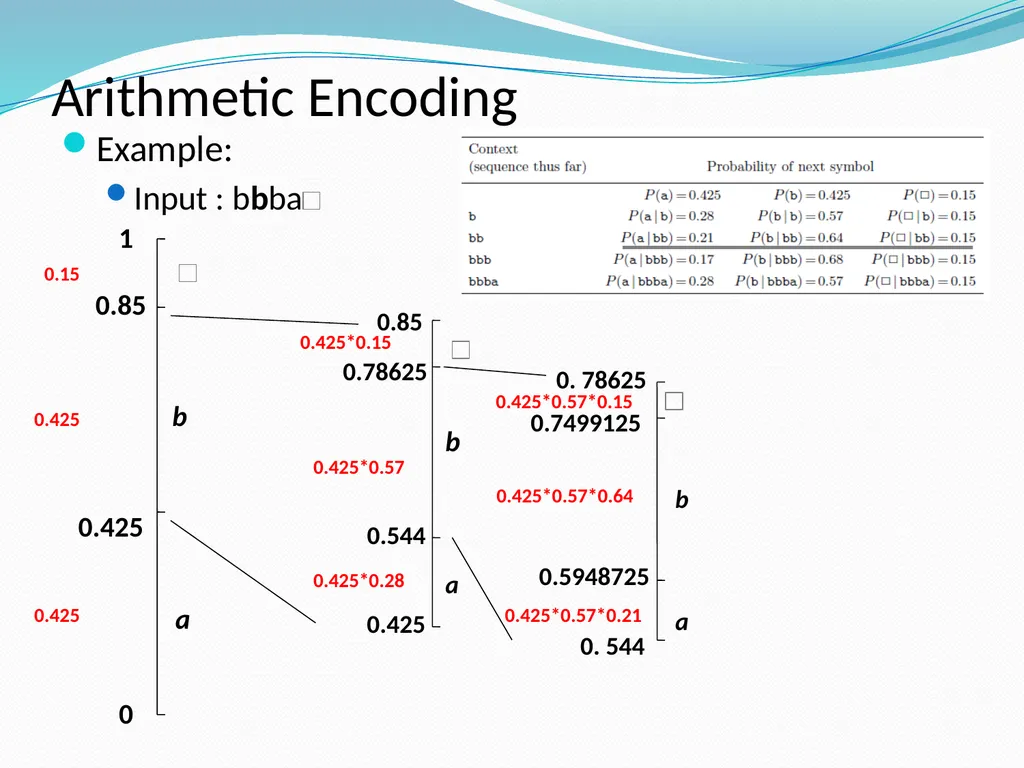
Arithmetic Encoding Example:
Input : bbba 0 1 0.425 0.85 a 0.425 0.15 0.425 0.85 0.425 0.544 0.78625 0.425*0.15 0.425*0.57 0.425*0.28 0. 544 0. 78625 0.425*0.57*0.15 0.425*0.57*0.64 0.5948725 0.7499125 a b 0.425*0.57*0.21 b b a<br>
Input : bbba 0 1 0.425 0.85 a 0.425 0.15 0.425 0.85 0.425 0.544 0.78625 0.425*0.15 0.425*0.57 0.425*0.28 0. 544 0. 78625 0.425*0.57*0.15 0.425*0.57*0.64 0.5948725 0.7499125 a b 0.425*0.57*0.21 b b a<br>
19
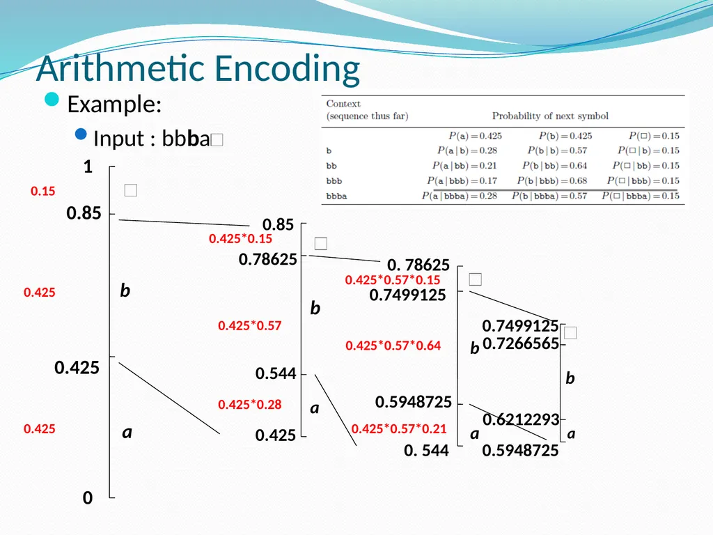
Arithmetic Encoding Example:
Input : bbba 0 1 0.425 0.85 a 0.425 0.15 0.425 0.85 0.425 0.544 0.78625 0.425*0.15 0.425*0.57 0.425*0.28 0. 544 0. 78625 0.425*0.57*0.15 0.425*0.57*0.64 0.5948725 0.7499125 a b 0.425*0.57*0.21 a b 0.5948725 0.7499125 b b a 0.7266565 0.6212293<br>
Input : bbba 0 1 0.425 0.85 a 0.425 0.15 0.425 0.85 0.425 0.544 0.78625 0.425*0.15 0.425*0.57 0.425*0.28 0. 544 0. 78625 0.425*0.57*0.15 0.425*0.57*0.64 0.5948725 0.7499125 a b 0.425*0.57*0.21 a b 0.5948725 0.7499125 b b a 0.7266565 0.6212293<br>
20
Arithmetic Encoding Example:
Input : bbba 20 0 1 0.425 0.85 a 0.425 0.15 0.425 0.85 0.425 0.544 0.78625 0.425*0.15 0.425*0.57 0.425*0.28 0. 544 0. 78625 0.425*0.57*0.15 0.425*0.57*0.64 0.5948725 0.7499125 a b 0.425*0.57*0.21 a b a b 0.5948725 0.7499125 0.6212293 0. 61727578 [0. 61727578,0.6212293) b b a 0.7266565 0.6212293<br>
Input : bbba 20 0 1 0.425 0.85 a 0.425 0.15 0.425 0.85 0.425 0.544 0.78625 0.425*0.15 0.425*0.57 0.425*0.28 0. 544 0. 78625 0.425*0.57*0.15 0.425*0.57*0.64 0.5948725 0.7499125 a b 0.425*0.57*0.21 a b a b 0.5948725 0.7499125 0.6212293 0. 61727578 [0. 61727578,0.6212293) b b a 0.7266565 0.6212293<br>
21
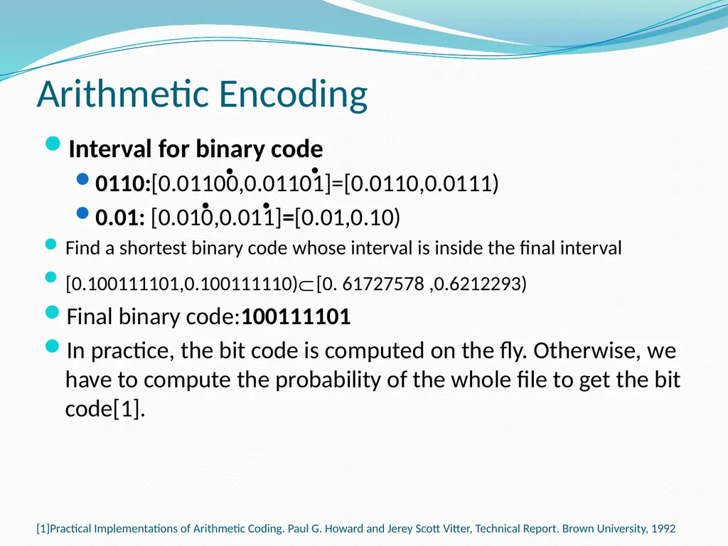
Arithmetic Encoding Interval for binary code
0110:[0.01100,0.01101]=[0.0110,0.0111)
0.01: [0.010,0.011]=[0.01,0.10)
Find a shortest binary code whose interval is inside the final interval
[0.100111101,0.100111110) [0. 61727578 ,0.6212293)
Final binary code:100111101
In practice, the bit code is computed on the fly. Otherwise, we have to compute the probability of the whole file to get the bit code[1]. [1]Practical Implementations of Arithmetic Coding. Paul G. Howard and Jerey Scott Vitter, Technical Report. Brown University, 1992<br>
0110:[0.01100,0.01101]=[0.0110,0.0111)
0.01: [0.010,0.011]=[0.01,0.10)
Find a shortest binary code whose interval is inside the final interval
[0.100111101,0.100111110) [0. 61727578 ,0.6212293)
Final binary code:100111101
In practice, the bit code is computed on the fly. Otherwise, we have to compute the probability of the whole file to get the bit code[1]. [1]Practical Implementations of Arithmetic Coding. Paul G. Howard and Jerey Scott Vitter, Technical Report. Brown University, 1992<br>
22
Arithmetic Decoding Example:
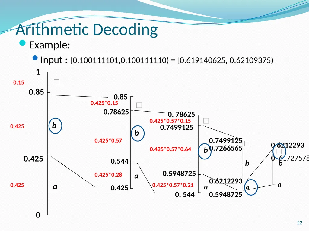
Input : [0.100111101,0.100111110) = [0.619140625, 0.62109375) 22 0 1 0.425 0.85 a 0.425 0.15 0.425 0.85 0.425 0.544 0.78625 0.425*0.15 0.425*0.57 0.425*0.28 0. 544 0. 78625 0.425*0.57*0.15 0.425*0.57*0.64 0.5948725 0.7499125 a b 0.425*0.57*0.21 a b a b 0.5948725 0.7499125 0.6212293 0. 61727578 b b a 0.7266565 0.6212293<br>
Input : [0.100111101,0.100111110) = [0.619140625, 0.62109375) 22 0 1 0.425 0.85 a 0.425 0.15 0.425 0.85 0.425 0.544 0.78625 0.425*0.15 0.425*0.57 0.425*0.28 0. 544 0. 78625 0.425*0.57*0.15 0.425*0.57*0.64 0.5948725 0.7499125 a b 0.425*0.57*0.21 a b a b 0.5948725 0.7499125 0.6212293 0. 61727578 b b a 0.7266565 0.6212293<br>
23
Outline Introduction
Overview of Huffman Coding
Arithmetic Coding
Encoding and Decoding
Probabilistic Model
(break)
Loss Analysis
Lempel-Ziv Coding
Summary<br>
Overview of Huffman Coding
Arithmetic Coding
Encoding and Decoding
Probabilistic Model
(break)
Loss Analysis
Lempel-Ziv Coding
Summary<br>
24
Why does it Work More bits are needed to express a number in a smaller interval
When a new symbol is encoded
Interval becomes smaller
High-prob symbol do not decrease interval size significantly, therefore need fewer bits than low-prob symbols
A good probabilistic model is important
The decoded messages will match the number of bits given by entropy, which for long messages is very close to optimal<br>
When a new symbol is encoded
Interval becomes smaller
High-prob symbol do not decrease interval size significantly, therefore need fewer bits than low-prob symbols
A good probabilistic model is important
The decoded messages will match the number of bits given by entropy, which for long messages is very close to optimal<br>
25
Separation between modeling and coding Given an interval [a,b] and a probability function P(x)
For any possible symbol x as the next symbol, the sub-interval [a’,b’] can be determined
Function P(x) could be adjusted at any point of time
P(x) can be a static distribution of all symbols
P(x) can also be a function of encountered symbols
The change of P(x) will not affect encode or decode
Since the same P(x) can be calculated in both encode and decode phase<br>
For any possible symbol x as the next symbol, the sub-interval [a’,b’] can be determined
Function P(x) could be adjusted at any point of time
P(x) can be a static distribution of all symbols
P(x) can also be a function of encountered symbols
The change of P(x) will not affect encode or decode
Since the same P(x) can be calculated in both encode and decode phase<br>
26
Choices of Probabilistic Model Two types of probabilistic models can be used
Static probabilistic model
Adaptive probabilistic model
Static probabilistic model
Preprocess the data and calculate symbol statistics
Calculated probabilities reflecting the occurance of each symbol in the whole data set<br>
Static probabilistic model
Adaptive probabilistic model
Static probabilistic model
Preprocess the data and calculate symbol statistics
Calculated probabilities reflecting the occurance of each symbol in the whole data set<br>
27
Choices of Probabilistic Model What if we have no idea about the distribution of incoming data?
Since the probabilities can change over time, we can make it predictive to meet the distribution of incoming data
Adaptive probabilistic model
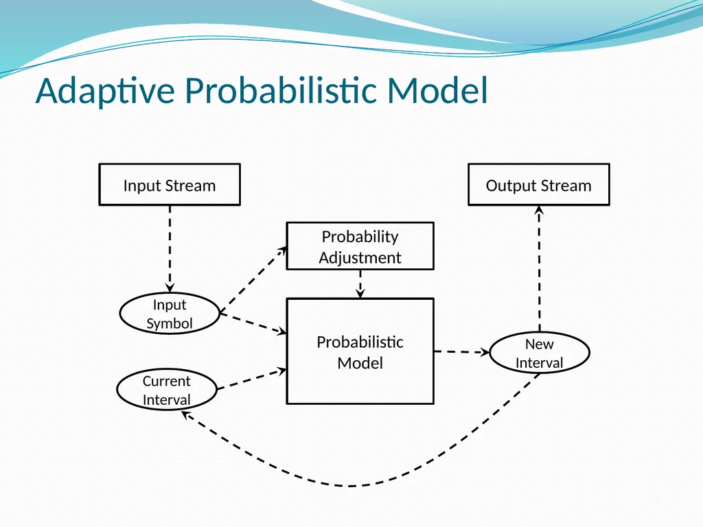
Give equal initial probability for each symbol
Adjust when a new symbol comes<br>
Since the probabilities can change over time, we can make it predictive to meet the distribution of incoming data
Adaptive probabilistic model
Give equal initial probability for each symbol
Adjust when a new symbol comes<br>
28
Adaptive Probabilistic Model<br>
29
Efficiency of Dynamic Probabilistic Model The amount of computation is linear to the input size
For a input string of length N
There are N rounds of probability adjustment
In each round, |A| probabilities are needed
In total, N|A| conditional probabilities are computed
The probabilities are computed only when the context actually encountered<br>
For a input string of length N
There are N rounds of probability adjustment
In each round, |A| probabilities are needed
In total, N|A| conditional probabilities are computed
The probabilities are computed only when the context actually encountered<br>
30
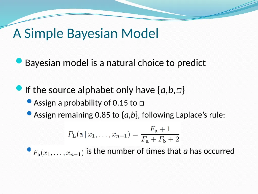
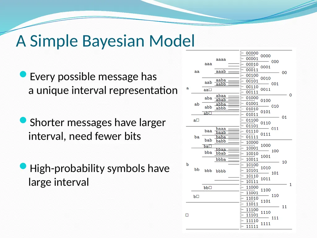
A Simple Bayesian Model Bayesian model is a natural choice to predict
If the source alphabet only have {a,b,□}
Assign a probability of 0.15 to □
Assign remaining 0.85 to {a,b}, following Laplace’s rule:
is the number of times that a has occurred<br>
If the source alphabet only have {a,b,□}
Assign a probability of 0.15 to □
Assign remaining 0.85 to {a,b}, following Laplace’s rule:
is the number of times that a has occurred<br>
31
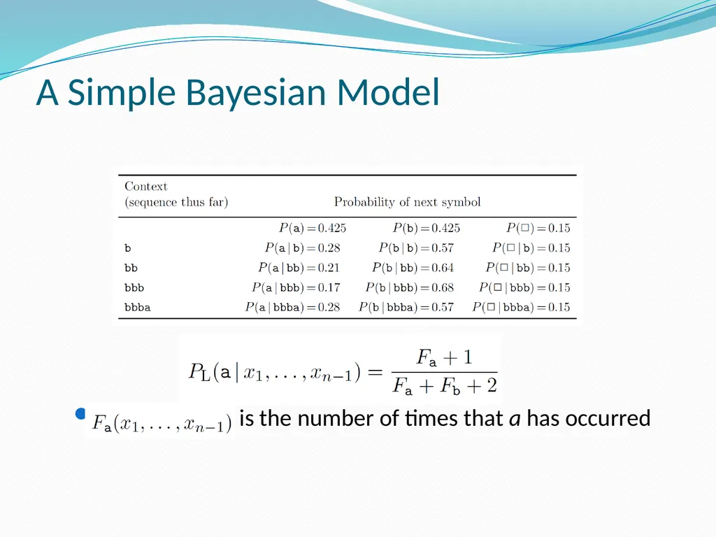
A Simple Bayesian Model is the number of times that a has occurred<br>
32
A Simple Bayesian Model Every possible message has
a unique interval representation
Shorter messages have larger interval, need fewer bits
High-probability symbols have large interval<br>
Shorter messages have larger interval, need fewer bits
High-probability symbols have large interval<br>
33
Flexibility of Arithmetic Code Can handle any source alphabet and encoded alphabet
The size of source alphabet and encoded alphabet can change over time
Simply divide interval into one more sub-interval when a new type of symbol comes
Can use any probability distribution, which can change utterly from context to context
Adaptive probabilistic model<br>
The size of source alphabet and encoded alphabet can change over time
Simply divide interval into one more sub-interval when a new type of symbol comes
Can use any probability distribution, which can change utterly from context to context
Adaptive probabilistic model<br>
34
Other Adaptive Probabilistic Model Symbol distribution changes over time
Symbols occurred too long ago have no help
distribution of recent symbols can help to predict
Count the frequency of last m symbols
Utilize context information
In most real-world cases, symbols have high correlation
Probability differs with different context information
Use the conditional probability of current context to predict<br>
Symbols occurred too long ago have no help
distribution of recent symbols can help to predict
Count the frequency of last m symbols
Utilize context information
In most real-world cases, symbols have high correlation
Probability differs with different context information
Use the conditional probability of current context to predict<br>
35
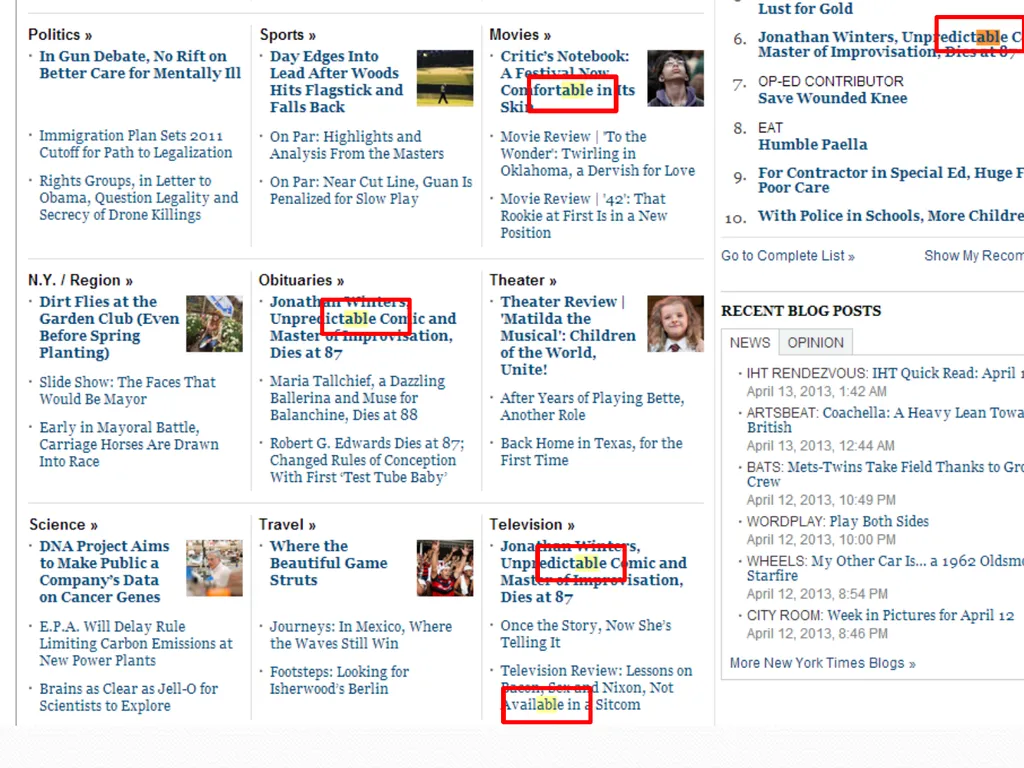
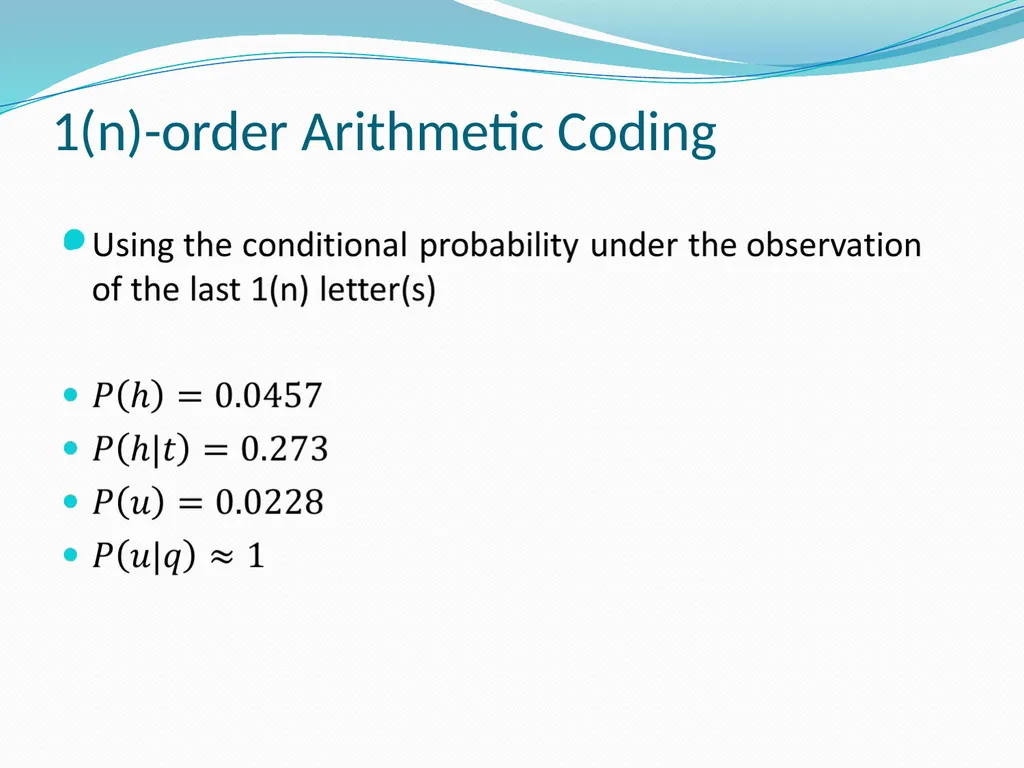
Context Information In English, the probability of h is relatively low. However, if the last letter is t, then the probability is very high.
See what is the next letter after abl in NewYork Times<br>
See what is the next letter after abl in NewYork Times<br>
36
1(n)-order Arithmetic Coding<br>
37
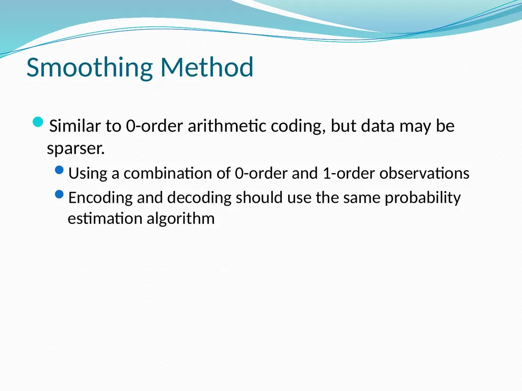
Smoothing Method Similar to 0-order arithmetic coding, but data may be sparser.
Using a combination of 0-order and 1-order observations
Encoding and decoding should use the same probability estimation algorithm<br>
Using a combination of 0-order and 1-order observations
Encoding and decoding should use the same probability estimation algorithm<br>
38
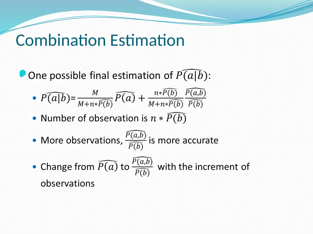
Combination Estimation<br>
39
Outline Introduction
Overview of Huffman Coding
Arithmetic Coding
Encoding and Decoding
Probabilistic Model
(break)
Loss Analysis
Lempel-Ziv Coding
Summary<br>
Overview of Huffman Coding
Arithmetic Coding
Encoding and Decoding
Probabilistic Model
(break)
Loss Analysis
Lempel-Ziv Coding
Summary<br>
40
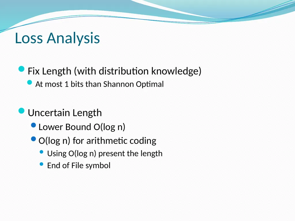
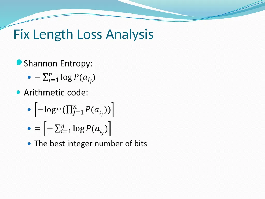
Loss Analysis Fix Length (with distribution knowledge)
At most 1 bits than Shannon Optimal
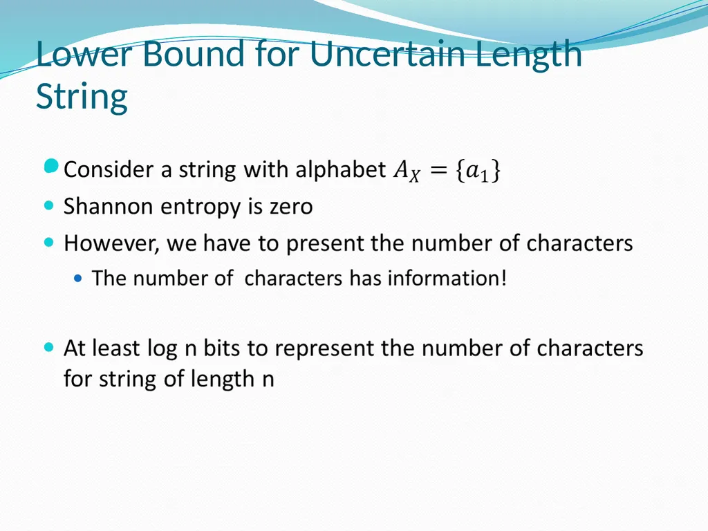
Uncertain Length
Lower Bound O(log n)
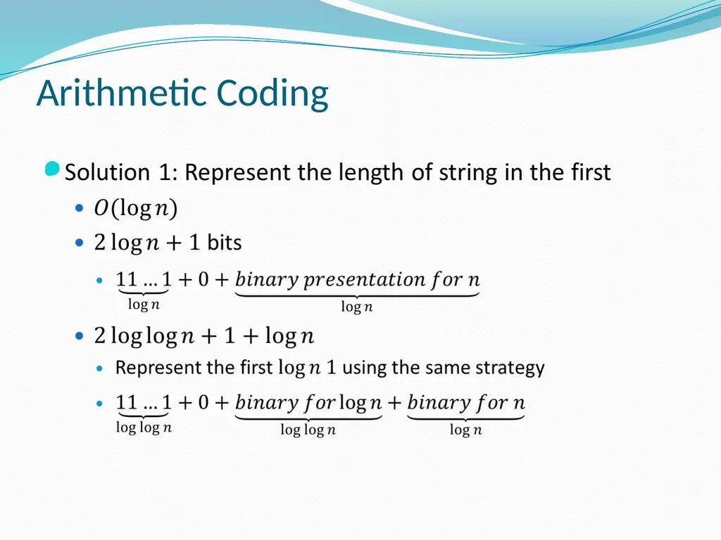
O(log n) for arithmetic coding
Using O(log n) present the length
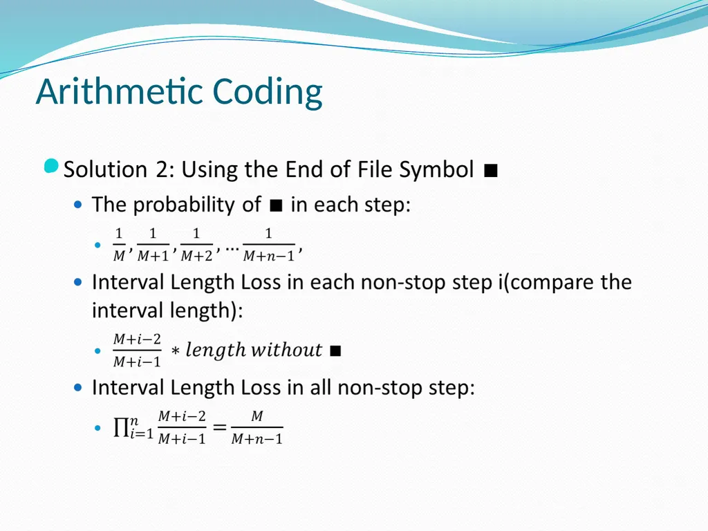
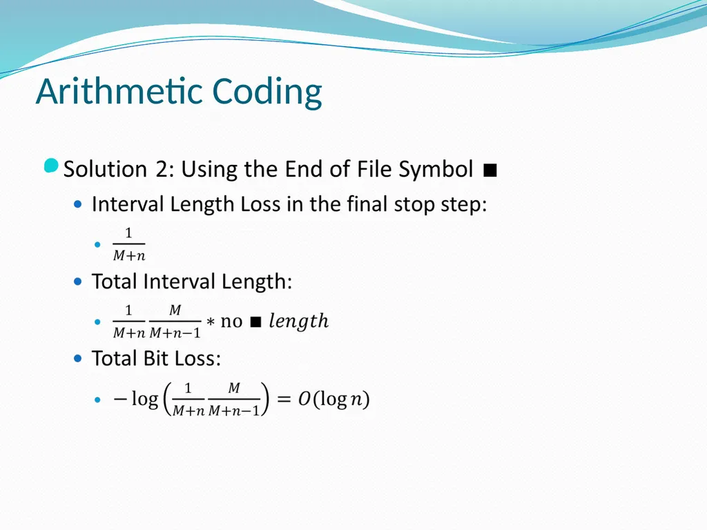
End of File symbol<br>
At most 1 bits than Shannon Optimal
Uncertain Length
Lower Bound O(log n)
O(log n) for arithmetic coding
Using O(log n) present the length
End of File symbol<br>
41
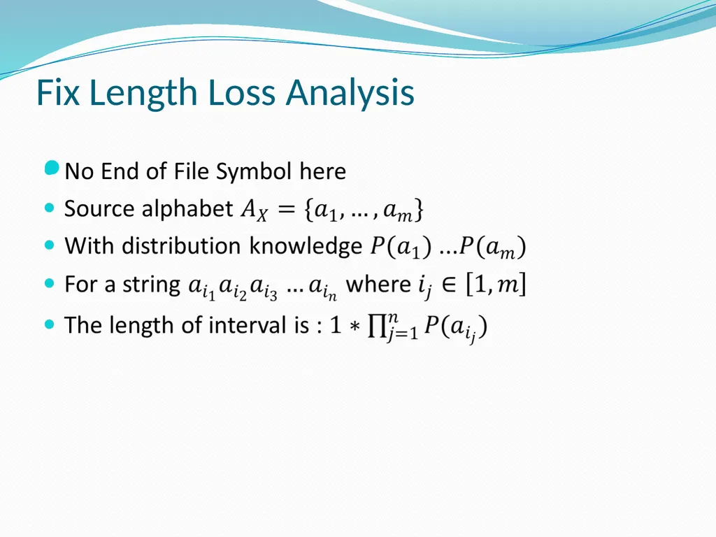
Fix Length Loss Analysis<br>
42
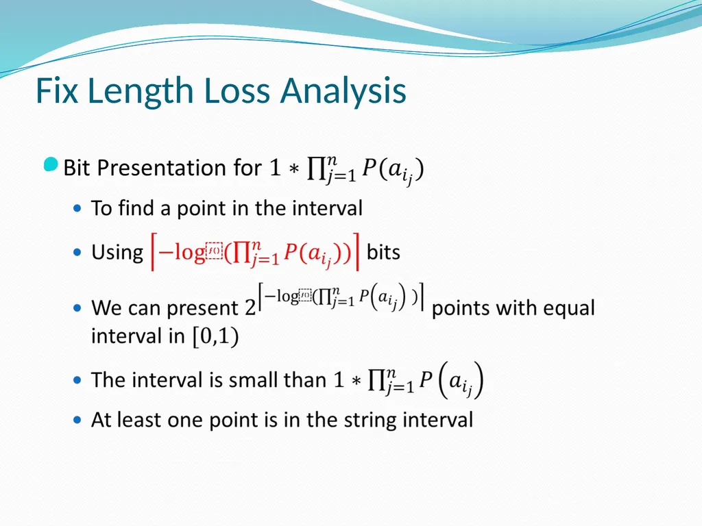
Fix Length Loss Analysis<br>
43
Fix Length Loss Analysis<br>
44
Lower Bound for Uncertain Length String<br>
45
Arithmetic Coding<br>
46
Arithmetic Coding<br>
47
Arithmetic Coding<br>
48
Outline Introduction
Overview of Huffman Coding
Arithmetic Coding
Encoding and Decoding
Probabilistic Model
(break)
Loss Analysis
Lempel-Ziv Coding
Summary<br>
Overview of Huffman Coding
Arithmetic Coding
Encoding and Decoding
Probabilistic Model
(break)
Loss Analysis
Lempel-Ziv Coding
Summary<br>
49
Introduction Lempel-Ziv coding is a lossless data compression algorithm
Algorithm is easy to implement
The compression is universal. It does not need to know any extra information before hand. The receiver does not need to know the table constructed by the transmitter as well
Belongs to the category of dictionary coders for lossless compression technique.<br>
Algorithm is easy to implement
The compression is universal. It does not need to know any extra information before hand. The receiver does not need to know the table constructed by the transmitter as well
Belongs to the category of dictionary coders for lossless compression technique.<br>
50
Applications Compression of data in most computers. zip , gzip , etc…
GIF images are compressed using the Lempel-Ziv encoding techniques to reduce the file size without decreasing the quality of the visual quality
It may also be used in PDF files<br>
GIF images are compressed using the Lempel-Ziv encoding techniques to reduce the file size without decreasing the quality of the visual quality
It may also be used in PDF files<br>
51
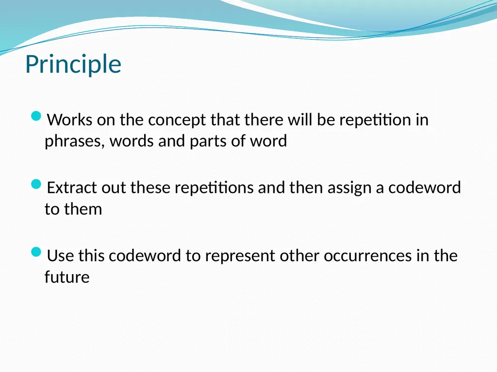
Principle Works on the concept that there will be repetition in phrases, words and parts of word
Extract out these repetitions and then assign a codeword to them
Use this codeword to represent other occurrences in the future<br>
Extract out these repetitions and then assign a codeword to them
Use this codeword to represent other occurrences in the future<br>
52
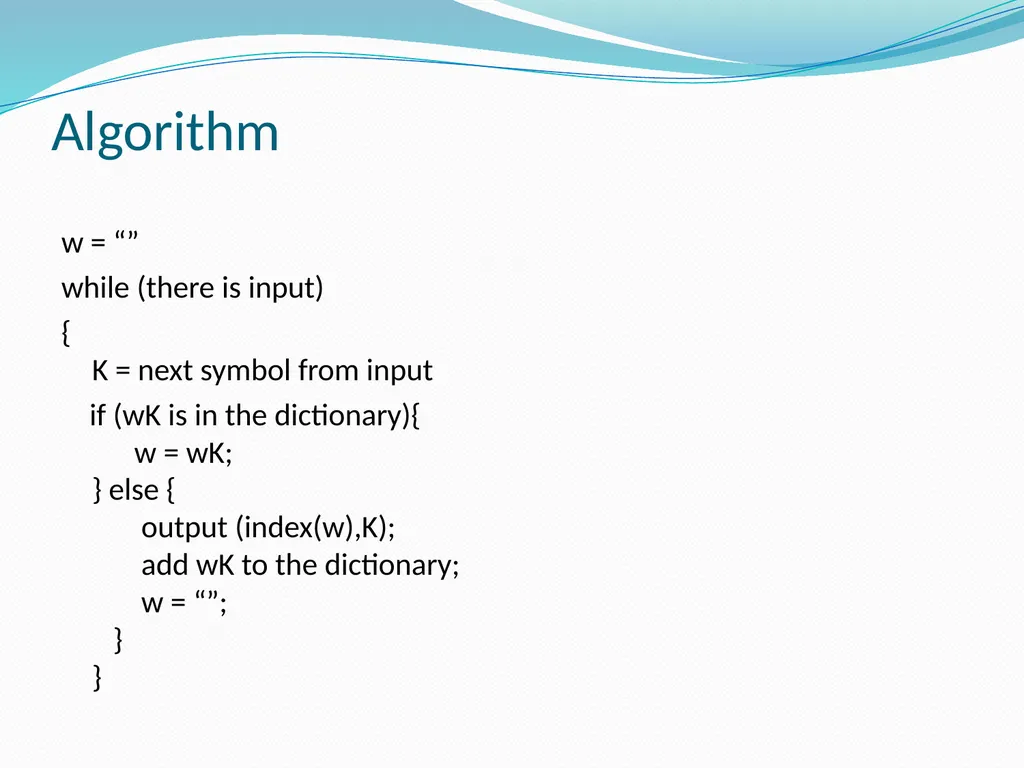
Algorithm w = “”
while (there is input)
{ K = next symbol from input
if (wK is in the dictionary){ w = wK; } else { output (index(w),K); add wK to the dictionary; w = “”; } }<br>
while (there is input)
{ K = next symbol from input
if (wK is in the dictionary){ w = wK; } else { output (index(w),K); add wK to the dictionary; w = “”; } }<br>
53
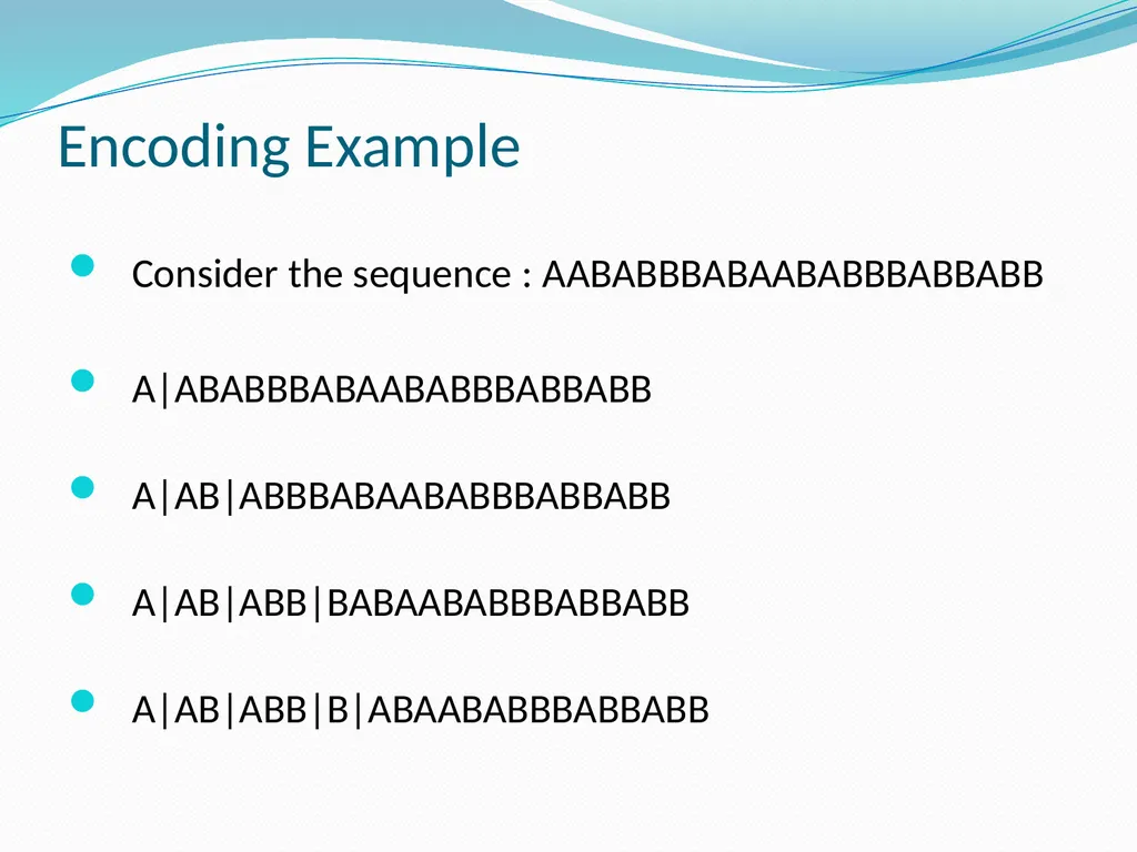
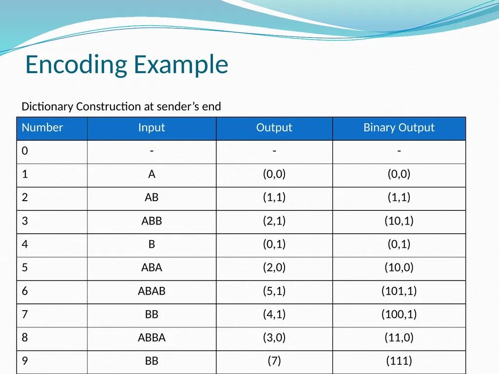
Encoding Example Consider the sequence : AABABBBABAABABBBABBABB
A|ABABBBABAABABBBABBABB
A|AB|ABBBABAABABBBABBABB
A|AB|ABB|BABAABABBBABBABB
A|AB|ABB|B|ABAABABBBABBABB<br>
A|ABABBBABAABABBBABBABB
A|AB|ABBBABAABABBBABBABB
A|AB|ABB|BABAABABBBABBABB
A|AB|ABB|B|ABAABABBBABBABB<br>
54
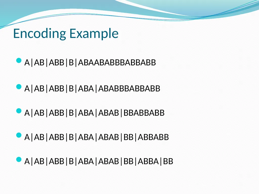
Encoding Example A|AB|ABB|B|ABAABABBBABBABB
A|AB|ABB|B|ABA|ABABBBABBABB
A|AB|ABB|B|ABA|ABAB|BBABBABB
A|AB|ABB|B|ABA|ABAB|BB|ABBABB
A|AB|ABB|B|ABA|ABAB|BB|ABBA|BB<br>
A|AB|ABB|B|ABA|ABABBBABBABB
A|AB|ABB|B|ABA|ABAB|BBABBABB
A|AB|ABB|B|ABA|ABAB|BB|ABBABB
A|AB|ABB|B|ABA|ABAB|BB|ABBA|BB<br>
55
Encoding Example Dictionary Construction at sender’s end<br>
56
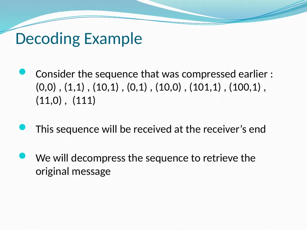
Decoding Example Consider the sequence that was compressed earlier :
(0,0) , (1,1) , (10,1) , (0,1) , (10,0) , (101,1) , (100,1) , (11,0) , (111)
This sequence will be received at the receiver’s end
We will decompress the sequence to retrieve the original message<br>
This sequence will be received at the receiver’s end
We will decompress the sequence to retrieve the original message<br>
57
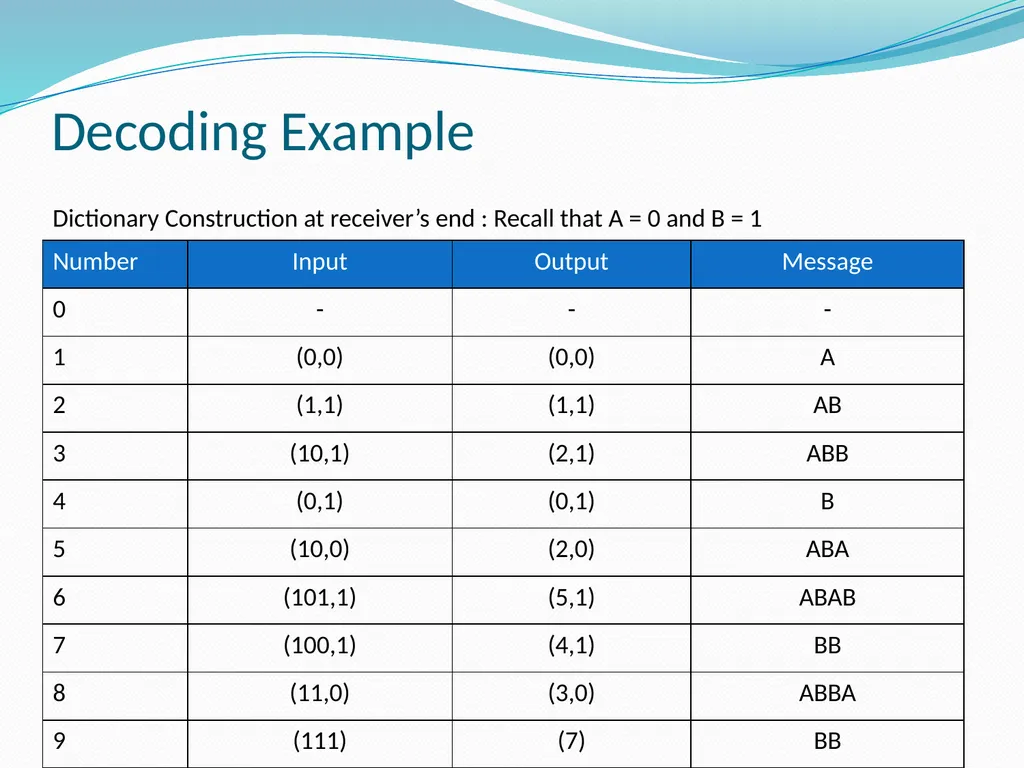
Decoding Example Dictionary Construction at receiver’s end : Recall that A = 0 and B = 1<br>
58
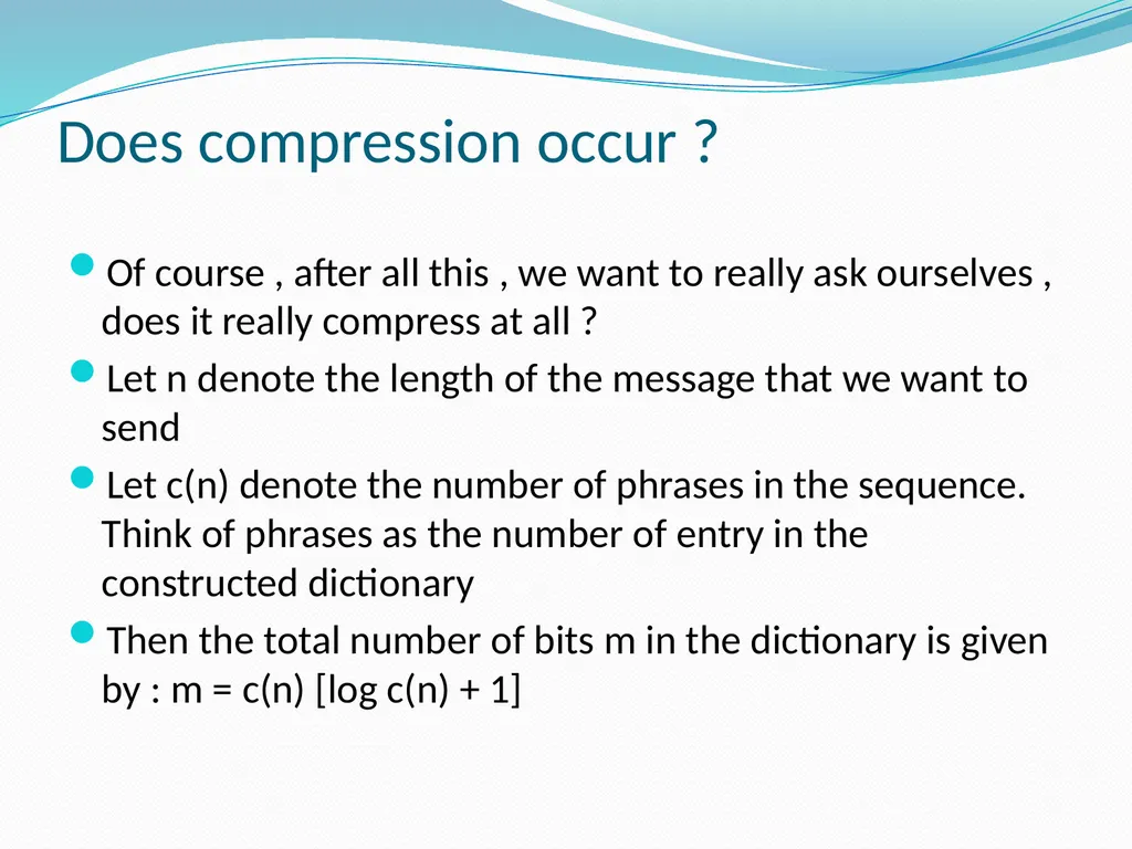
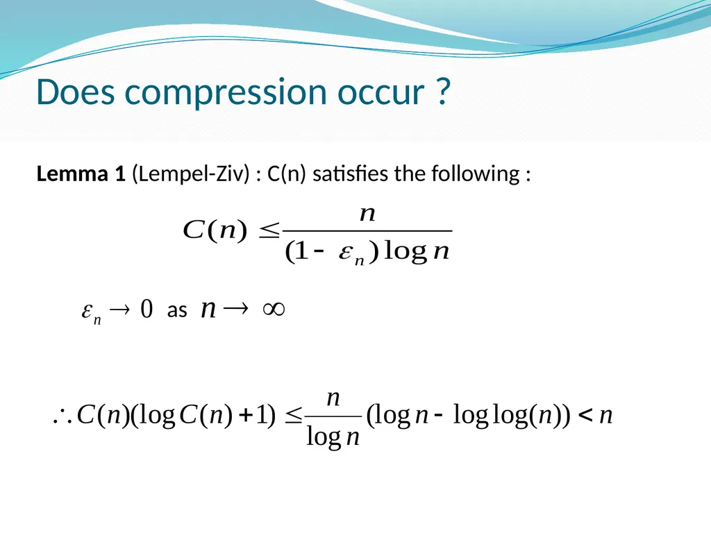
Does compression occur ? Of course , after all this , we want to really ask ourselves , does it really compress at all ?
Let n denote the length of the message that we want to send
Let c(n) denote the number of phrases in the sequence. Think of phrases as the number of entry in the constructed dictionary
Then the total number of bits m in the dictionary is given by : m = c(n) [log c(n) + 1]<br>
Let n denote the length of the message that we want to send
Let c(n) denote the number of phrases in the sequence. Think of phrases as the number of entry in the constructed dictionary
Then the total number of bits m in the dictionary is given by : m = c(n) [log c(n) + 1]<br>
59
Does compression occur ? Lemma 1 (Lempel-Ziv) : C(n) satisfies the following : as<br>
60
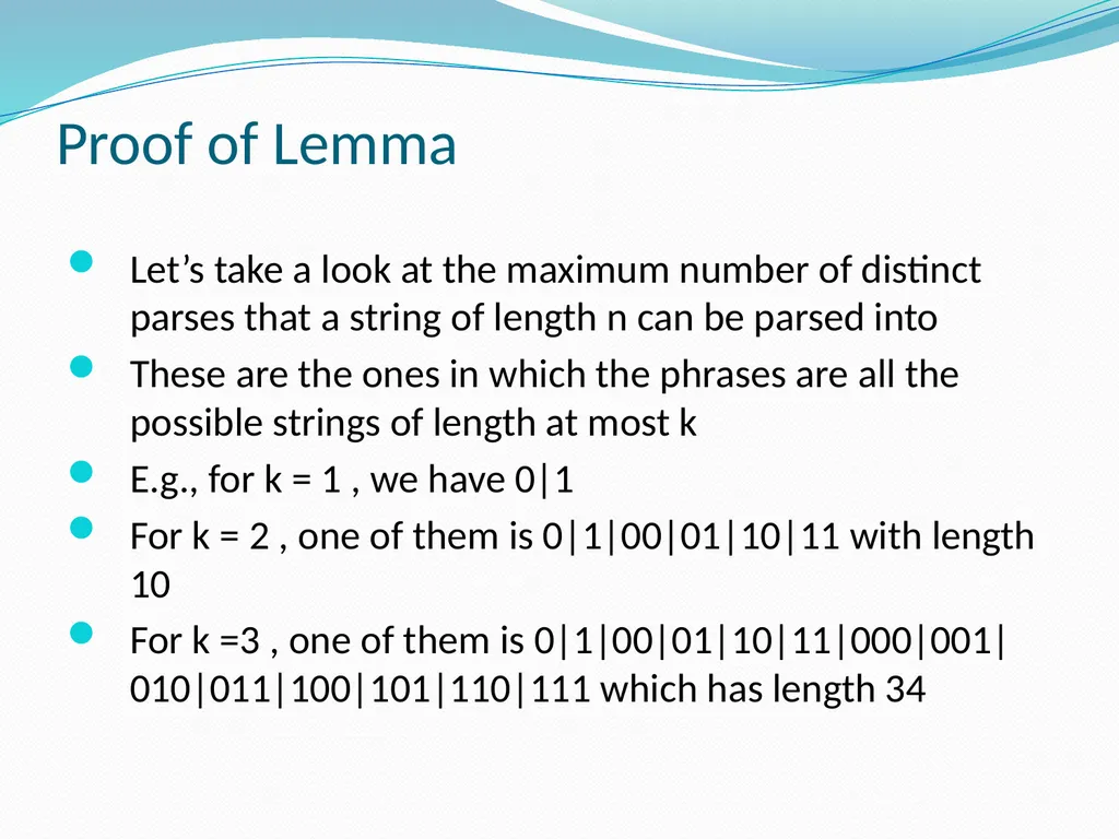
Proof of Lemma Let’s take a look at the maximum number of distinct parses that a string of length n can be parsed into
These are the ones in which the phrases are all the possible strings of length at most k
E.g., for k = 1 , we have 0|1
For k = 2 , one of them is 0|1|00|01|10|11 with length 10
For k =3 , one of them is 0|1|00|01|10|11|000|001|010|011|100|101|110|111 which has length 34<br>
These are the ones in which the phrases are all the possible strings of length at most k
E.g., for k = 1 , we have 0|1
For k = 2 , one of them is 0|1|00|01|10|11 with length 10
For k =3 , one of them is 0|1|00|01|10|11|000|001|010|011|100|101|110|111 which has length 34<br>
61
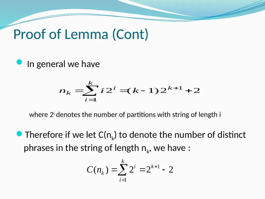
Proof of Lemma (Cont) In general we have
Therefore if we let C(nk) to denote the number of distinct phrases in the string of length nk, we have : where 2i denotes the number of partitions with string of length i<br>
Therefore if we let C(nk) to denote the number of distinct phrases in the string of length nk, we have : where 2i denotes the number of partitions with string of length i<br>
62
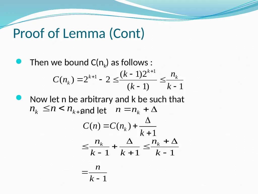
Proof of Lemma (Cont) Then we bound C(nk) as follows :
Now let n be arbitrary and k be such that and let<br>
Now let n be arbitrary and k be such that and let<br>
63
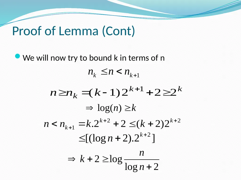
Proof of Lemma (Cont) We will now try to bound k in terms of n<br>
64
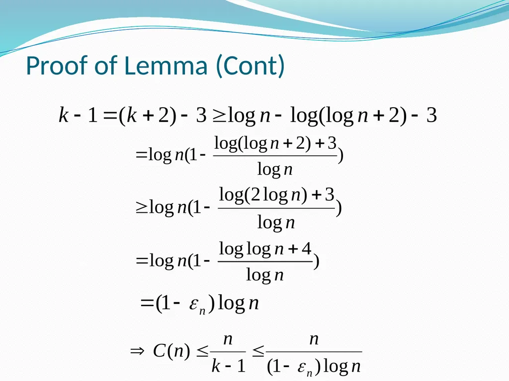
Proof of Lemma (Cont)<br>
65
Weakness of Lempel-Ziv Generally efficient for long messages or files
When short messages or messages that are too random, we might end up sending more bits than contained in the original message<br>
When short messages or messages that are too random, we might end up sending more bits than contained in the original message<br>
66
Outline Introduction
Overview of Huffman Coding
Arithmetic Coding
Encoding and Decoding
Probabilistic Model
(break)
Loss Analysis
Lempel-Ziv Coding
Summary<br>
Overview of Huffman Coding
Arithmetic Coding
Encoding and Decoding
Probabilistic Model
(break)
Loss Analysis
Lempel-Ziv Coding
Summary<br>
67
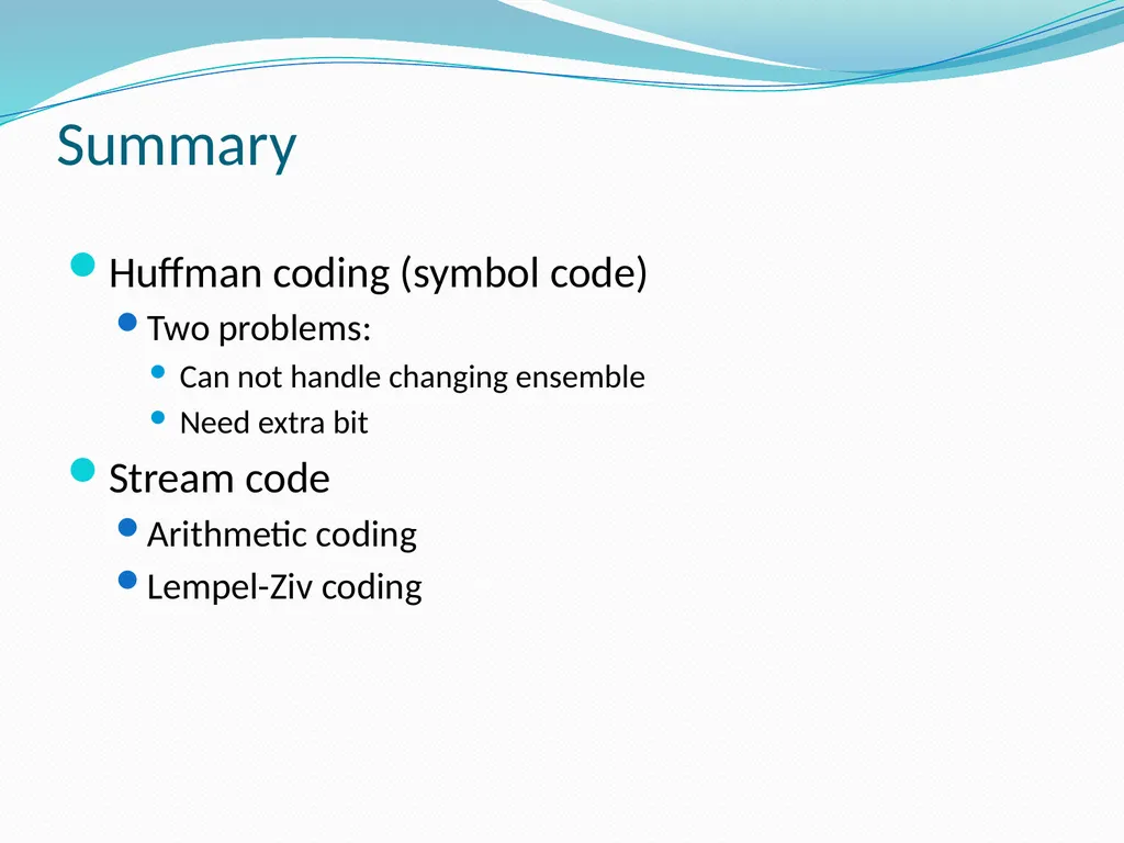
Summary Huffman coding (symbol code)
Two problems:
Can not handle changing ensemble
Need extra bit
Stream code
Arithmetic coding
Lempel-Ziv coding<br>
Two problems:
Can not handle changing ensemble
Need extra bit
Stream code
Arithmetic coding
Lempel-Ziv coding<br>
68
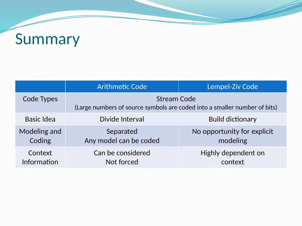
Summary<br>
69
References http://www-math.mit.edu/~shor/PAM/lempel_ziv_notes.pdf
http://www.cmlab.csie.ntu.edu.tw/~itct/slide/Data_Compression_Lempel-Ziv_Coding.pdf
Information Theory, Inference, and Learning Algorithms. David J.C. Maykay. Cambridge University Press<br>
http://www.cmlab.csie.ntu.edu.tw/~itct/slide/Data_Compression_Lempel-Ziv_Coding.pdf
Information Theory, Inference, and Learning Algorithms. David J.C. Maykay. Cambridge University Press<br>
70
Q & A<br>