
The Dual of the Linear Programing Problem The
PT
Published · 29 slides · 0 views

1 / 1

Description
The Dual of the Linear Programing Problem The Duality of a Linear Programming Problem One of the most important discoveries in the early development of linear programming was the concept of duality. The dual Problem is an LP defined
Related Topics
Share
Embed code
Download this presentation From Below
"The Dual of the Linear Programing Problem The" is the property of its rightful owner. Permission is granted to download and print the materials on this website for personal, non-commercial use only, and to display it on your personal computer provided you do not modify the materials and that you retain all copyright notices contained in the materials. By downloading content from our website, you accept the terms of this agreement.
Presentation Transcript
01
The Dual of the Linear Programing Problem<br>
02
The Duality of a Linear Programming Problem One of the most important discoveries in the early development of linear programming was the concept of duality.
The dual Problem is an LP defined systematically from the primal (original) LP model.
Every linear programming problem is associated with another linear programming problem called the dual.<br>
The dual Problem is an LP defined systematically from the primal (original) LP model.
Every linear programming problem is associated with another linear programming problem called the dual.<br>
03
The relationships between the dual problem and the original problem (called the primal) prove to be extremely useful in a variety of ways.
The primal represents a resource case and the dual represents a recourse valuation. The Duality of a LPP Cont’d<br>
The primal represents a resource case and the dual represents a recourse valuation. The Duality of a LPP Cont’d<br>
04
Duality in LLP Cont’d The purpose of the dual problem is to provide insight into the original problem and to help solve it more efficiently. In particular, the dual problem can be used to:
Determine the sensitivity of the optimal solution to changes in the problem parameters, such as the coefficients in the objective function or the constraints.
Obtain bounds on the optimal value of the original problem.
Identify variables that are not part of the optimal solution, but are important in determining the optimal solution.<br>
Determine the sensitivity of the optimal solution to changes in the problem parameters, such as the coefficients in the objective function or the constraints.
Obtain bounds on the optimal value of the original problem.
Identify variables that are not part of the optimal solution, but are important in determining the optimal solution.<br>
05
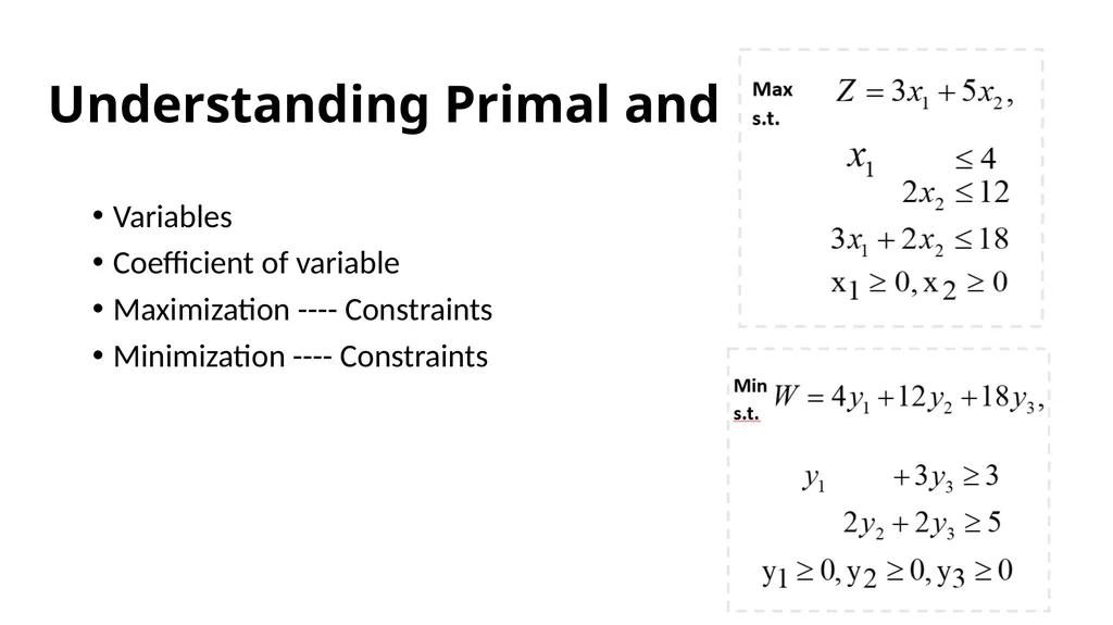
Understanding Primal and Dual Variables
Coefficient of variable
Maximization ---- Constraints
Minimization ---- Constraints<br>
Coefficient of variable
Maximization ---- Constraints
Minimization ---- Constraints<br>
06
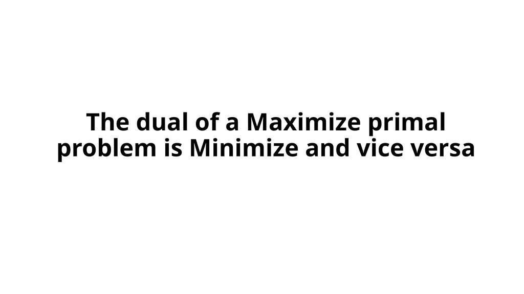
The dual of a Maximize primal problem is Minimize and vice versa<br>
07
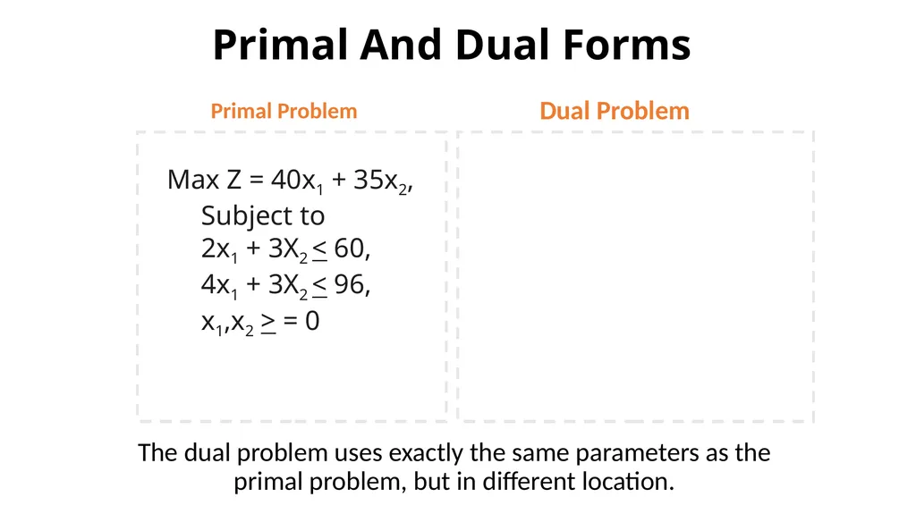
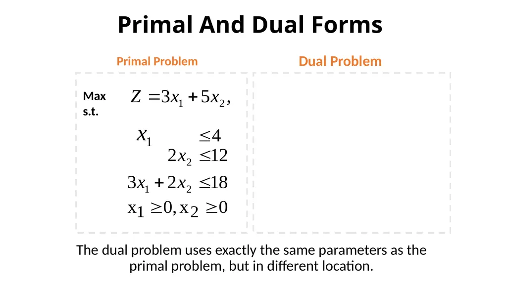
Primal Problem Dual Problem Primal And Dual Forms The dual problem uses exactly the same parameters as the primal problem, but in different location. Max Z = 40x1 + 35x2,
Subject to
2x1 + 3X2 < 60,
4x1 + 3X2 < 96,
x1,x2 > = 0<br>
Subject to
2x1 + 3X2 < 60,
4x1 + 3X2 < 96,
x1,x2 > = 0<br>
08
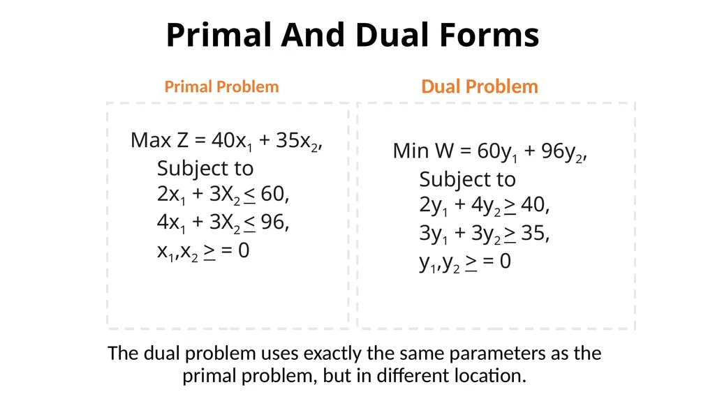
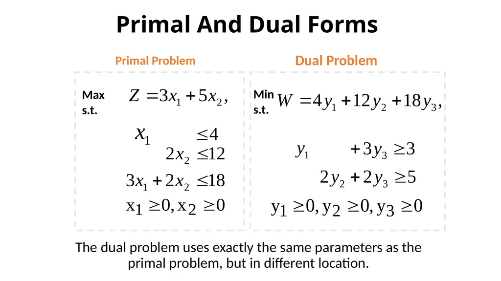
Primal Problem Dual Problem Primal And Dual Forms The dual problem uses exactly the same parameters as the primal problem, but in different location. Max Z = 40x1 + 35x2,
Subject to
2x1 + 3X2 < 60,
4x1 + 3X2 < 96,
x1,x2 > = 0 Min W = 60y1 + 96y2,
Subject to
2y1 + 4y2 > 40,
3y1 + 3y2 > 35,
y1,y2 > = 0<br>
Subject to
2x1 + 3X2 < 60,
4x1 + 3X2 < 96,
x1,x2 > = 0 Min W = 60y1 + 96y2,
Subject to
2y1 + 4y2 > 40,
3y1 + 3y2 > 35,
y1,y2 > = 0<br>
09
Max
s.t. Primal Problem Dual Problem Primal And Dual Forms The dual problem uses exactly the same parameters as the primal problem, but in different location.<br>
s.t. Primal Problem Dual Problem Primal And Dual Forms The dual problem uses exactly the same parameters as the primal problem, but in different location.<br>
10
Max
s.t. Min
s.t. Primal Problem Dual Problem Primal And Dual Forms The dual problem uses exactly the same parameters as the primal problem, but in different location.<br>
s.t. Min
s.t. Primal Problem Dual Problem Primal And Dual Forms The dual problem uses exactly the same parameters as the primal problem, but in different location.<br>
11
The dual of a dual problem is the primal problem<br>
12
Min
s.t. Primal Problem Dual Problem Primal And Dual Forms The dual problem uses exactly the same parameters as the primal problem, but in different location.<br>
s.t. Primal Problem Dual Problem Primal And Dual Forms The dual problem uses exactly the same parameters as the primal problem, but in different location.<br>
13
Max
s.t. Min
s.t. Primal Problem Dual Problem Primal And Dual Forms The dual problem uses exactly the same parameters as the primal problem, but in different location.<br>
s.t. Min
s.t. Primal Problem Dual Problem Primal And Dual Forms The dual problem uses exactly the same parameters as the primal problem, but in different location.<br>
14
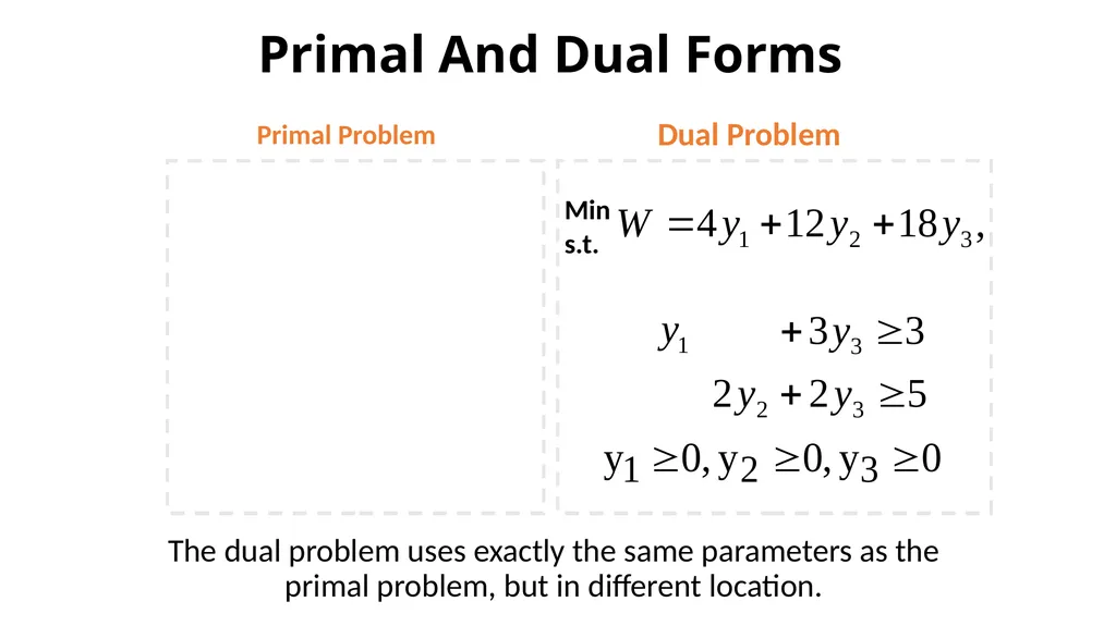
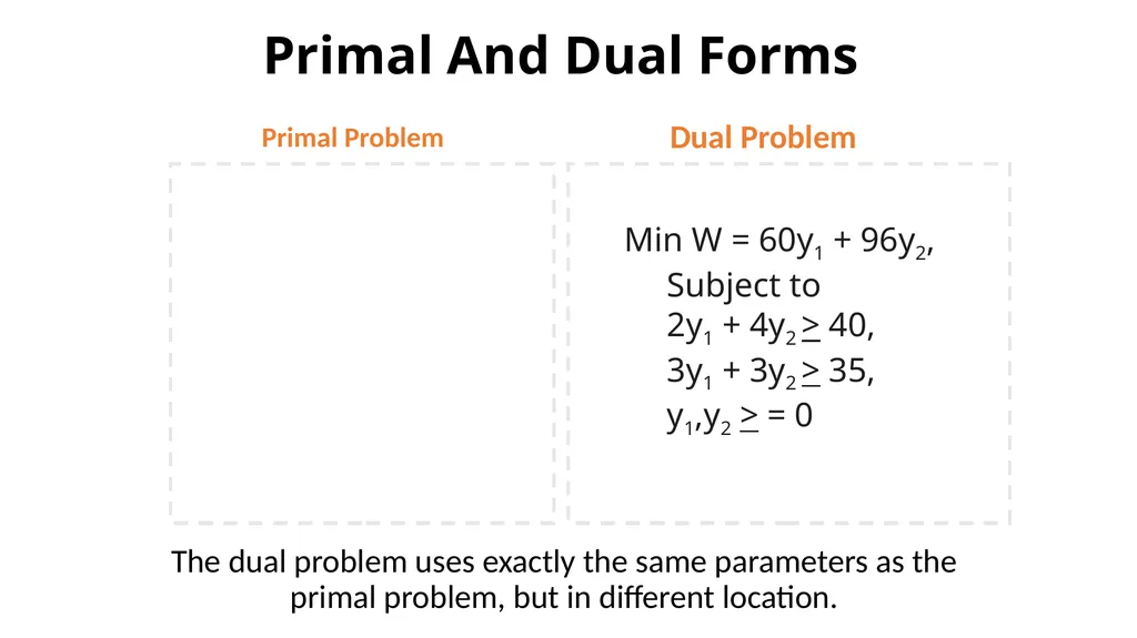
Primal Problem Dual Problem Primal And Dual Forms The dual problem uses exactly the same parameters as the primal problem, but in different location. Min W = 60y1 + 96y2,
Subject to
2y1 + 4y2 > 40,
3y1 + 3y2 > 35,
y1,y2 > = 0<br>
Subject to
2y1 + 4y2 > 40,
3y1 + 3y2 > 35,
y1,y2 > = 0<br>
15
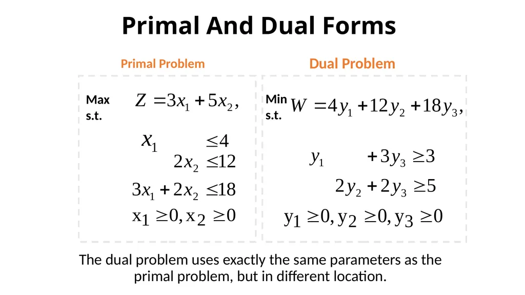
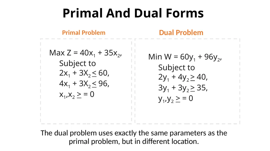
Primal Problem Dual Problem Primal And Dual Forms The dual problem uses exactly the same parameters as the primal problem, but in different location. Max Z = 40x1 + 35x2,
Subject to
2x1 + 3X2 < 60,
4x1 + 3X2 < 96,
x1,x2 > = 0 Min W = 60y1 + 96y2,
Subject to
2y1 + 4y2 > 40,
3y1 + 3y2 > 35,
y1,y2 > = 0<br>
Subject to
2x1 + 3X2 < 60,
4x1 + 3X2 < 96,
x1,x2 > = 0 Min W = 60y1 + 96y2,
Subject to
2y1 + 4y2 > 40,
3y1 + 3y2 > 35,
y1,y2 > = 0<br>
16
Strong Duality Vs. Weak Duality<br>
17
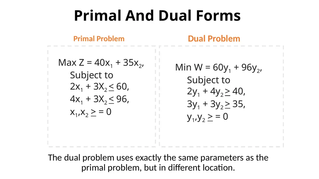
Primal Problem Dual Problem Primal And Dual Forms The dual problem uses exactly the same parameters as the primal problem, but in different location. Max Z = 40x1 + 35x2,
Subject to
2x1 + 3X2 < 60,
4x1 + 3X2 < 96,
x1,x2 > = 0 Min W = 60y1 + 96y2,
Subject to
2y1 + 4y2 > 40,
3y1 + 3y2 > 35,
y1,y2 > = 0<br>
Subject to
2x1 + 3X2 < 60,
4x1 + 3X2 < 96,
x1,x2 > = 0 Min W = 60y1 + 96y2,
Subject to
2y1 + 4y2 > 40,
3y1 + 3y2 > 35,
y1,y2 > = 0<br>
18
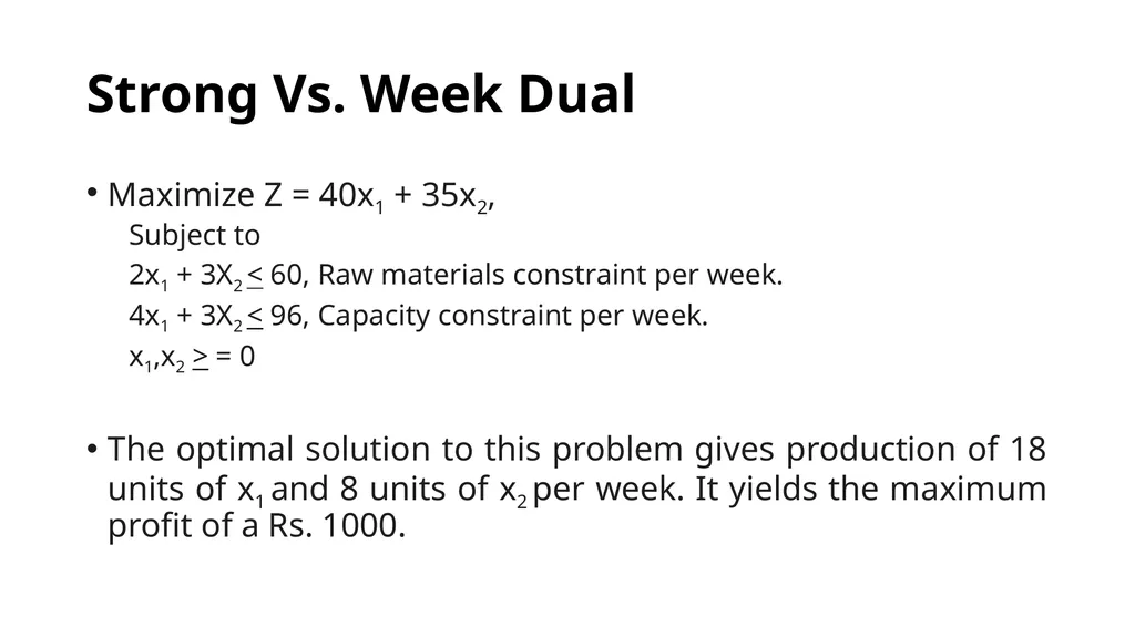
Strong Vs. Week Dual Maximize Z = 40x1 + 35x2,
Subject to
2x1 + 3X2 < 60, Raw materials constraint per week.
4x1 + 3X2 < 96, Capacity constraint per week.
x1,x2 > = 0
The optimal solution to this problem gives production of 18 units of x1 and 8 units of x2 per week. It yields the maximum profit of a Rs. 1000.<br>
Subject to
2x1 + 3X2 < 60, Raw materials constraint per week.
4x1 + 3X2 < 96, Capacity constraint per week.
x1,x2 > = 0
The optimal solution to this problem gives production of 18 units of x1 and 8 units of x2 per week. It yields the maximum profit of a Rs. 1000.<br>
19
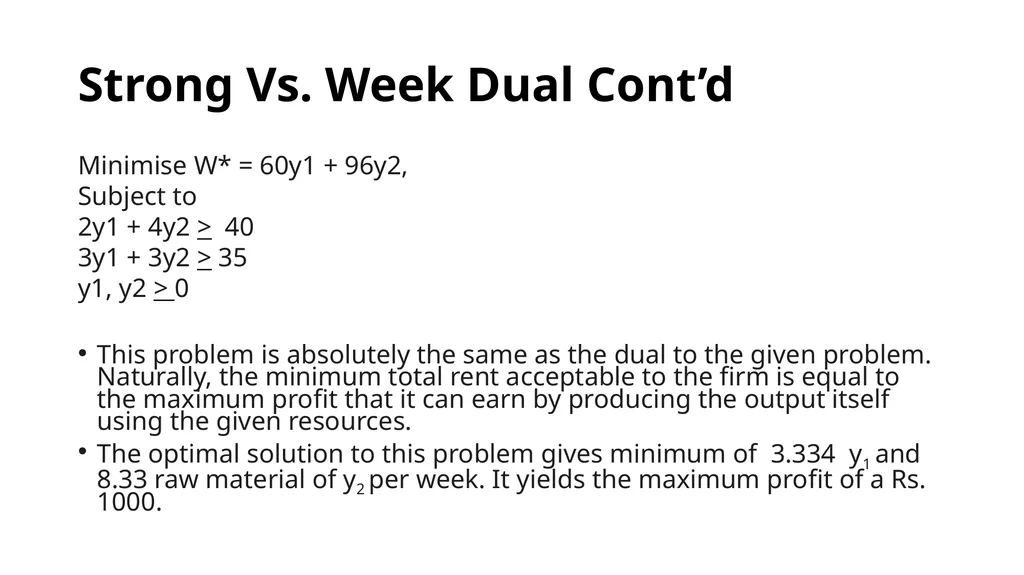
Strong Vs. Week Dual Cont’d Minimise W* = 60y1 + 96y2,
Subject to
2y1 + 4y2 > 40
3y1 + 3y2 > 35
y1, y2 > 0
This problem is absolutely the same as the dual to the given problem. Naturally, the minimum total rent acceptable to the firm is equal to the maximum profit that it can earn by producing the output itself using the given resources.
The optimal solution to this problem gives minimum of 3.334 y1 and 8.33 raw material of y2 per week. It yields the maximum profit of a Rs. 1000.<br>
Subject to
2y1 + 4y2 > 40
3y1 + 3y2 > 35
y1, y2 > 0
This problem is absolutely the same as the dual to the given problem. Naturally, the minimum total rent acceptable to the firm is equal to the maximum profit that it can earn by producing the output itself using the given resources.
The optimal solution to this problem gives minimum of 3.334 y1 and 8.33 raw material of y2 per week. It yields the maximum profit of a Rs. 1000.<br>
20
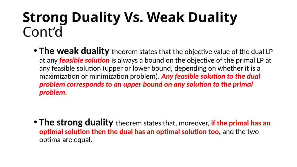
Strong Duality Vs. Weak Duality Cont’d The weak duality theorem states that the objective value of the dual LP at any feasible solution is always a bound on the objective of the primal LP at any feasible solution (upper or lower bound, depending on whether it is a maximization or minimization problem). Any feasible solution to the dual problem corresponds to an upper bound on any solution to the primal problem.
The strong duality theorem states that, moreover, if the primal has an optimal solution then the dual has an optimal solution too, and the two optima are equal.<br>
The strong duality theorem states that, moreover, if the primal has an optimal solution then the dual has an optimal solution too, and the two optima are equal.<br>
21
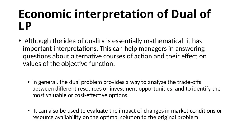
Economic interpretation of Dual of LP Although the idea of duality is essentially mathematical, it has important interpretations. This can help managers in answering questions about alternative courses of action and their effect on values of the objective function.
In general, the dual problem provides a way to analyze the trade-offs between different resources or investment opportunities, and to identify the most valuable or cost-effective options.
It can also be used to evaluate the impact of changes in market conditions or resource availability on the optimal solution to the original problem<br>
In general, the dual problem provides a way to analyze the trade-offs between different resources or investment opportunities, and to identify the most valuable or cost-effective options.
It can also be used to evaluate the impact of changes in market conditions or resource availability on the optimal solution to the original problem<br>
22
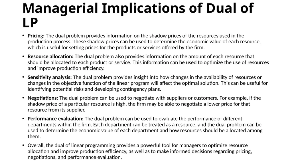
Managerial Implications of Dual of LP Pricing: The dual problem provides information on the shadow prices of the resources used in the production process. These shadow prices can be used to determine the economic value of each resource, which is useful for setting prices for the products or services offered by the firm.
Resource allocation: The dual problem also provides information on the amount of each resource that should be allocated to each product or service. This information can be used to optimize the use of resources and improve production efficiency.
Sensitivity analysis: The dual problem provides insight into how changes in the availability of resources or changes in the objective function of the linear program will affect the optimal solution. This can be useful for identifying potential risks and developing contingency plans.
Negotiations: The dual problem can be used to negotiate with suppliers or customers. For example, if the shadow price of a particular resource is high, the firm may be able to negotiate a lower price for that resource from its supplier.
Performance evaluation: The dual problem can be used to evaluate the performance of different departments within the firm. Each department can be treated as a resource, and the dual problem can be used to determine the economic value of each department and how resources should be allocated among them.
Overall, the dual of linear programming provides a powerful tool for managers to optimize resource allocation and improve production efficiency, as well as to make informed decisions regarding pricing, negotiations, and performance evaluation.<br>
Resource allocation: The dual problem also provides information on the amount of each resource that should be allocated to each product or service. This information can be used to optimize the use of resources and improve production efficiency.
Sensitivity analysis: The dual problem provides insight into how changes in the availability of resources or changes in the objective function of the linear program will affect the optimal solution. This can be useful for identifying potential risks and developing contingency plans.
Negotiations: The dual problem can be used to negotiate with suppliers or customers. For example, if the shadow price of a particular resource is high, the firm may be able to negotiate a lower price for that resource from its supplier.
Performance evaluation: The dual problem can be used to evaluate the performance of different departments within the firm. Each department can be treated as a resource, and the dual problem can be used to determine the economic value of each department and how resources should be allocated among them.
Overall, the dual of linear programming provides a powerful tool for managers to optimize resource allocation and improve production efficiency, as well as to make informed decisions regarding pricing, negotiations, and performance evaluation.<br>
23
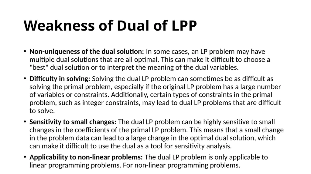
Weakness of Dual of LPP Non-uniqueness of the dual solution: In some cases, an LP problem may have multiple dual solutions that are all optimal. This can make it difficult to choose a "best" dual solution or to interpret the meaning of the dual variables.
Difficulty in solving: Solving the dual LP problem can sometimes be as difficult as solving the primal problem, especially if the original LP problem has a large number of variables or constraints. Additionally, certain types of constraints in the primal problem, such as integer constraints, may lead to dual LP problems that are difficult to solve.
Sensitivity to small changes: The dual LP problem can be highly sensitive to small changes in the coefficients of the primal LP problem. This means that a small change in the problem data can lead to a large change in the optimal dual solution, which can make it difficult to use the dual as a tool for sensitivity analysis.
Applicability to non-linear problems: The dual LP problem is only applicable to linear programming problems. For non-linear programming problems.<br>
Difficulty in solving: Solving the dual LP problem can sometimes be as difficult as solving the primal problem, especially if the original LP problem has a large number of variables or constraints. Additionally, certain types of constraints in the primal problem, such as integer constraints, may lead to dual LP problems that are difficult to solve.
Sensitivity to small changes: The dual LP problem can be highly sensitive to small changes in the coefficients of the primal LP problem. This means that a small change in the problem data can lead to a large change in the optimal dual solution, which can make it difficult to use the dual as a tool for sensitivity analysis.
Applicability to non-linear problems: The dual LP problem is only applicable to linear programming problems. For non-linear programming problems.<br>
24
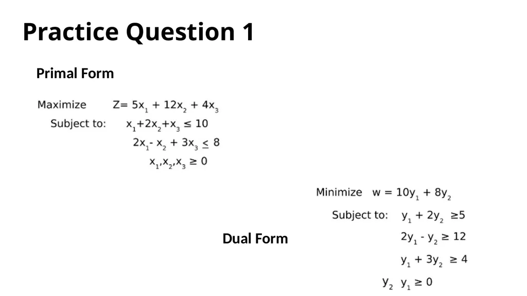
Primal Form Dual Form Practice Question 1<br>
25
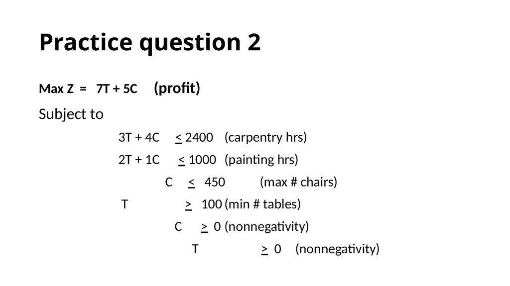
Practice question 2 Max Z = 7T + 5C (profit)
Subject to
3T + 4C < 2400 (carpentry hrs)
2T + 1C < 1000 (painting hrs)
C < 450 (max # chairs)
T > 100 (min # tables)
C > 0 (nonnegativity)
T > 0 (nonnegativity)<br>
Subject to
3T + 4C < 2400 (carpentry hrs)
2T + 1C < 1000 (painting hrs)
C < 450 (max # chairs)
T > 100 (min # tables)
C > 0 (nonnegativity)
T > 0 (nonnegativity)<br>
26
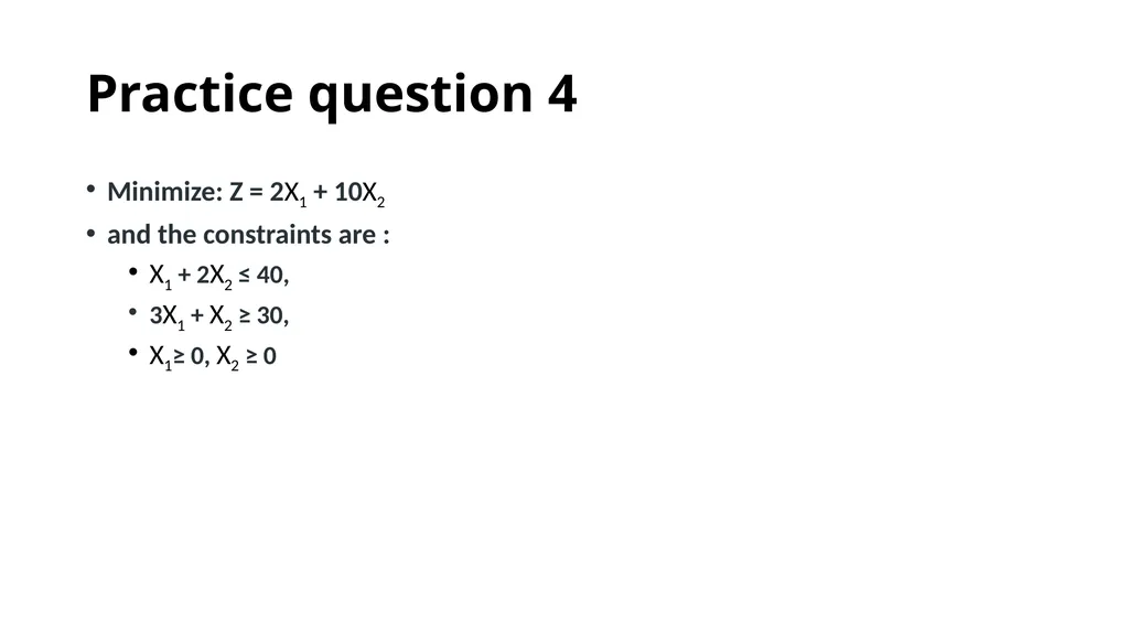
Practice question 4 Minimize: Z = 2X1 + 10X2
and the constraints are :
X1 + 2X2 ≤ 40,
3X1 + X2 ≥ 30,
X1≥ 0, X2 ≥ 0<br>
and the constraints are :
X1 + 2X2 ≤ 40,
3X1 + X2 ≥ 30,
X1≥ 0, X2 ≥ 0<br>
27
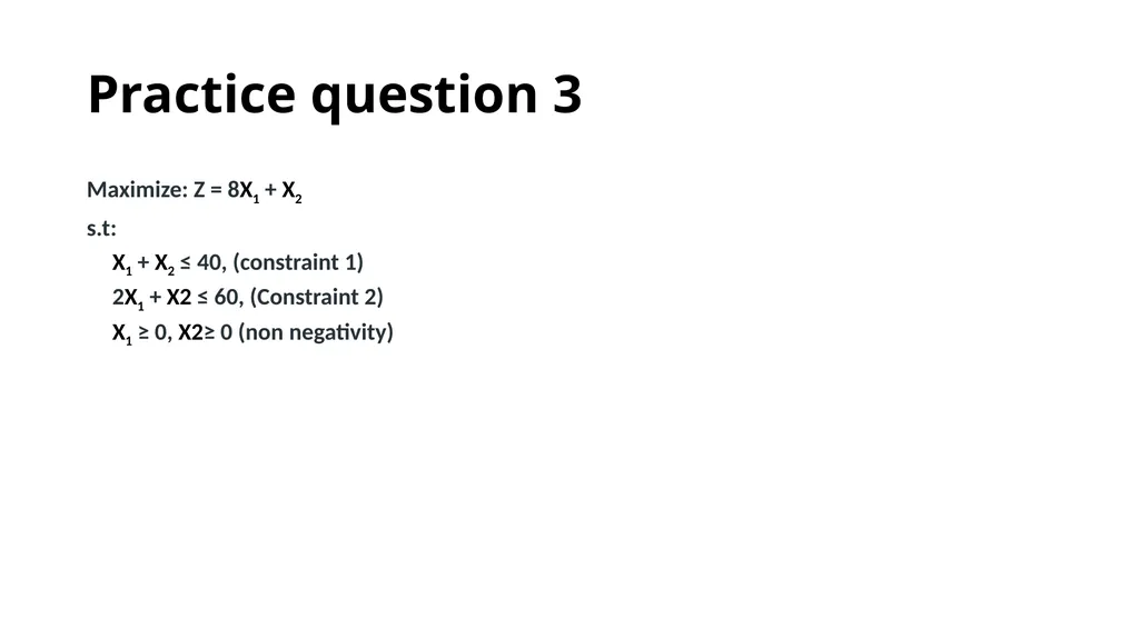
Practice question 3 Maximize: Z = 8X1 + X2
s.t:
X1 + X2 ≤ 40, (constraint 1)
2X1 + X2 ≤ 60, (Constraint 2)
X1 ≥ 0, X2≥ 0 (non negativity)<br>
s.t:
X1 + X2 ≤ 40, (constraint 1)
2X1 + X2 ≤ 60, (Constraint 2)
X1 ≥ 0, X2≥ 0 (non negativity)<br>
28
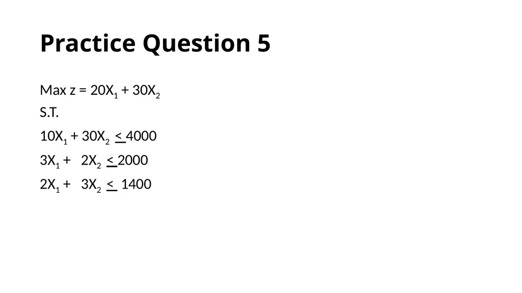
Practice Question 5 Max z = 20X1 + 30X2
S.T.
10X1 + 30X2 < 4000
3X1 + 2X2 < 2000
2X1 + 3X2 < 1400<br>
S.T.
10X1 + 30X2 < 4000
3X1 + 2X2 < 2000
2X1 + 3X2 < 1400<br>
29
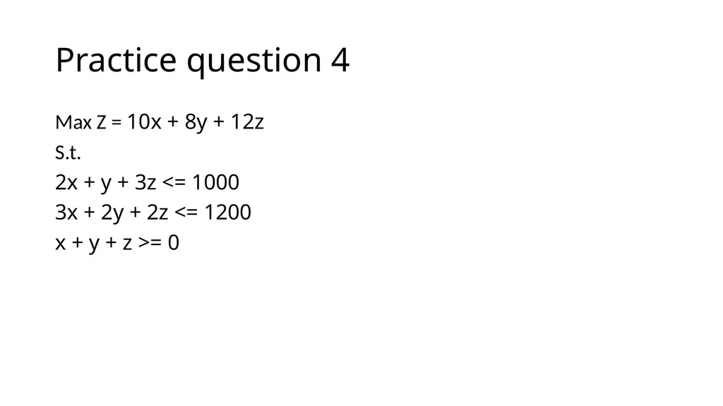
Practice question 4 Max Z = 10x + 8y + 12z
S.t.
2x + y + 3z <= 1000
3x + 2y + 2z <= 1200
x + y + z >= 0<br>
S.t.
2x + y + 3z <= 1000
3x + 2y + 2z <= 1200
x + y + z >= 0<br>