The Open Economy Revisited: The Mundell-Fleming
Author : natalia-silvester | Published Date : 2025-11-08
Description: The Open Economy Revisited The MundellFleming Model and the ExchangeRate Regime Macroeconomics N Gregory Mankiw 2019 Worth Publishers all rights reserved IN THIS CHAPTER YOU WILL LEARN About the MundellFleming model ISLM for the
Presentation Embed Code
Download Presentation
Download
Presentation The PPT/PDF document
"The Open Economy Revisited: The Mundell-Fleming" is the property of its rightful owner.
Permission is granted to download and print the materials on this website for personal, non-commercial use only,
and to display it on your personal computer provided you do not modify the materials and that you retain all
copyright notices contained in the materials. By downloading content from our website, you accept the terms of
this agreement.
Transcript:The Open Economy Revisited: The Mundell-Fleming:
The Open Economy Revisited: The Mundell-Fleming Model and the Exchange-Rate Regime Macroeconomics N. Gregory Mankiw © 2019 Worth Publishers, all rights reserved IN THIS CHAPTER, YOU WILL LEARN: About the Mundell–Fleming model (IS–LM for the small open economy) About causes and effects of interest rate differentials Arguments for fixed versus floating exchange rates How to derive the aggregate demand curve for a small open economy The Mundell-Fleming model Key assumption: Small open economy with perfect capital mobility. r = r* Goods market equilibrium—the IS* curve: where e = nominal exchange rate = foreign currency per unit domestic currency The IS* curve: Goods market equilibrium The IS* curve is drawn for a given value of r*. Intuition for the slope: The LM* curve: Money market equilibrium The LM* curve: is drawn for a given value of r*. is vertical because, given r*, there is only one value of Y that equates money demand with supply, regardless of e. Equilibrium in the Mundell-Fleming model Floating and fixed exchange rates In a system of floating exchange rates, e is allowed to fluctuate in response to changing economic conditions. In contrast, under fixed exchange rates, the central bank trades domestic for foreign currency at a predetermined price. Next, policy analysis: in a floating exchange rate system in a fixed exchange rate system Fiscal policy under floating exchange rates At any given value of e, a fiscal expansion increases Y, shifting IS* to the right. Results: Δe > 0, ΔY = 0 Lessons about fiscal policy In a small open economy with perfect capital mobility, fiscal policy cannot affect real GDP. Crowding out closed economy: Fiscal policy crowds out investment by causing the interest rate to rise. small open economy: Fiscal policy crowds out net exports by causing the exchange rate to appreciate. Monetary policy under floating exchange rates An increase in M shifts LM* right because Y must rise to restore equilibrium in the money market. Results: Δe < 0, ΔY > 0 Lessons about monetary policy Monetary policy affects output by affecting the components of aggregate demand: closed economy: M → r → I → Y small open economy: M → e → NX → Y Expansionary monetary policy does not raise world aggregate demand; it merely shifts demand from foreign to domestic products. So, the increases in domestic income and employment are at the expense of losses abroad. Trade policy under floating