THEORETICAL DISTRIBUTION Dr. Gavisiddappa Gadag Introduction: In case of population the values of variables are distributed according to some definite probability law which can be expressed mathematically and the corresponding probability
"THEORETICAL DISTRIBUTION Dr. Gavisiddappa Gadag" is the property of its rightful owner. Permission is granted to
download and print the materials on this website for personal, non-commercial use only, and to display it
on your personal computer provided you do not modify the materials and that you retain all copyright
notices contained in the materials. By downloading content from our website, you accept the terms of this
agreement.
Presentation Transcript
01
THEORETICAL DISTRIBUTION Dr. Gavisiddappa Gadag<br>
02
Introduction: In case of population the values of variables are distributed according to some definite probability law which can be expressed mathematically and the corresponding probability distribution is known as theoretical probability distribution.
Probability Distribution: Probability distribution is nothing but distribution of total probability to different points or intervals.
The probability distributions which are not obtained by actual observations or experiments but are mathematically deduced on certain assumptions are theoretical probability distribution.<br>
03
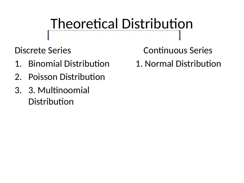
Theoretical Distribution Discrete Series
Binomial Distribution
Poisson Distribution
3. Multinoomial Distribution Continuous Series
1. Normal Distribution<br>
04
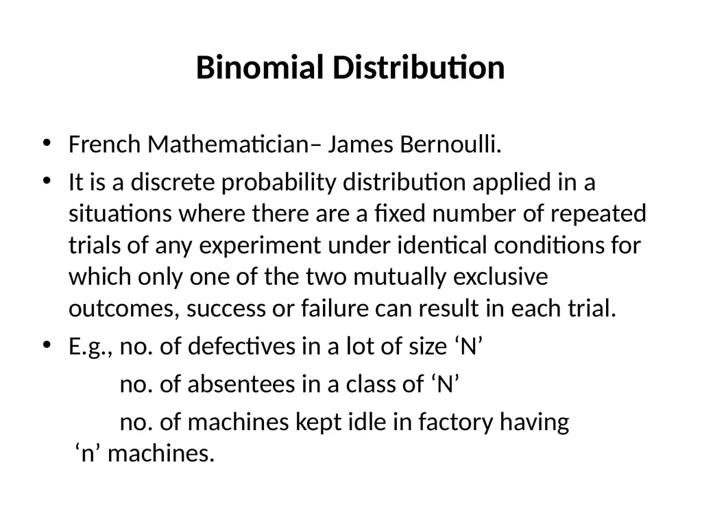
Binomial Distribution French Mathematician– James Bernoulli.
It is a discrete probability distribution applied in a situations where there are a fixed number of repeated trials of any experiment under identical conditions for which only one of the two mutually exclusive outcomes, success or failure can result in each trial.
E.g., no. of defectives in a lot of size ‘N’
no. of absentees in a class of ‘N’
no. of machines kept idle in factory having ‘n’ machines.<br>
05
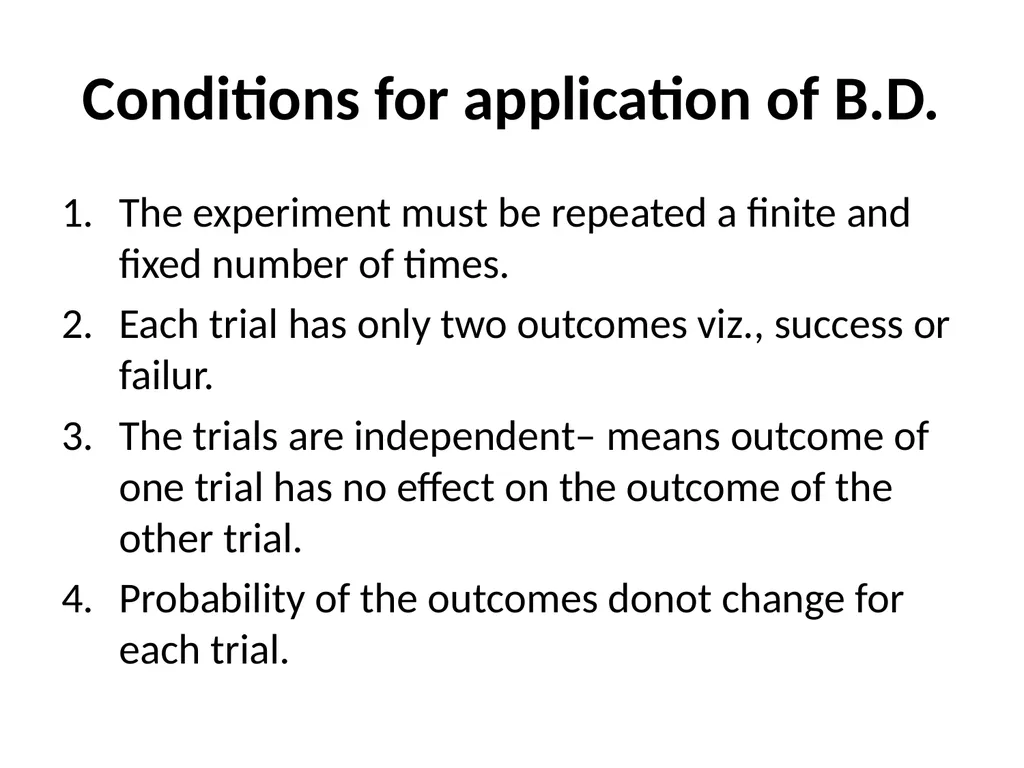
Conditions for application of B.D. The experiment must be repeated a finite and fixed number of times.
Each trial has only two outcomes viz., success or failur.
The trials are independent– means outcome of one trial has no effect on the outcome of the other trial.
Probability of the outcomes donot change for each trial.<br>
06
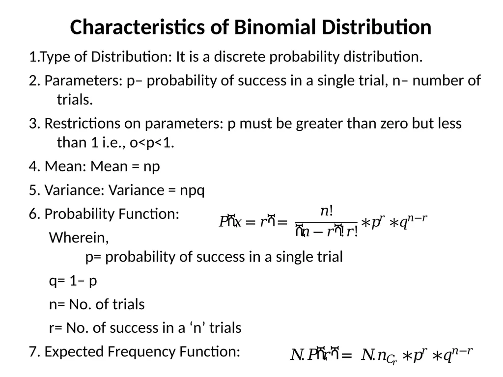
Characteristics of Binomial Distribution 1.Type of Distribution: It is a discrete probability distribution.
2. Parameters: p– probability of success in a single trial, n– number of trials.
3. Restrictions on parameters: p must be greater than zero but less than 1 i.e., o<p<1.
4. Mean: Mean = np
5. Variance: Variance = npq
6. Probability Function:
Wherein, p= probability of success in a single trial
q= 1– p
n= No. of trials
r= No. of success in a ‘n’ trials
7. Expected Frequency Function:<br>
07
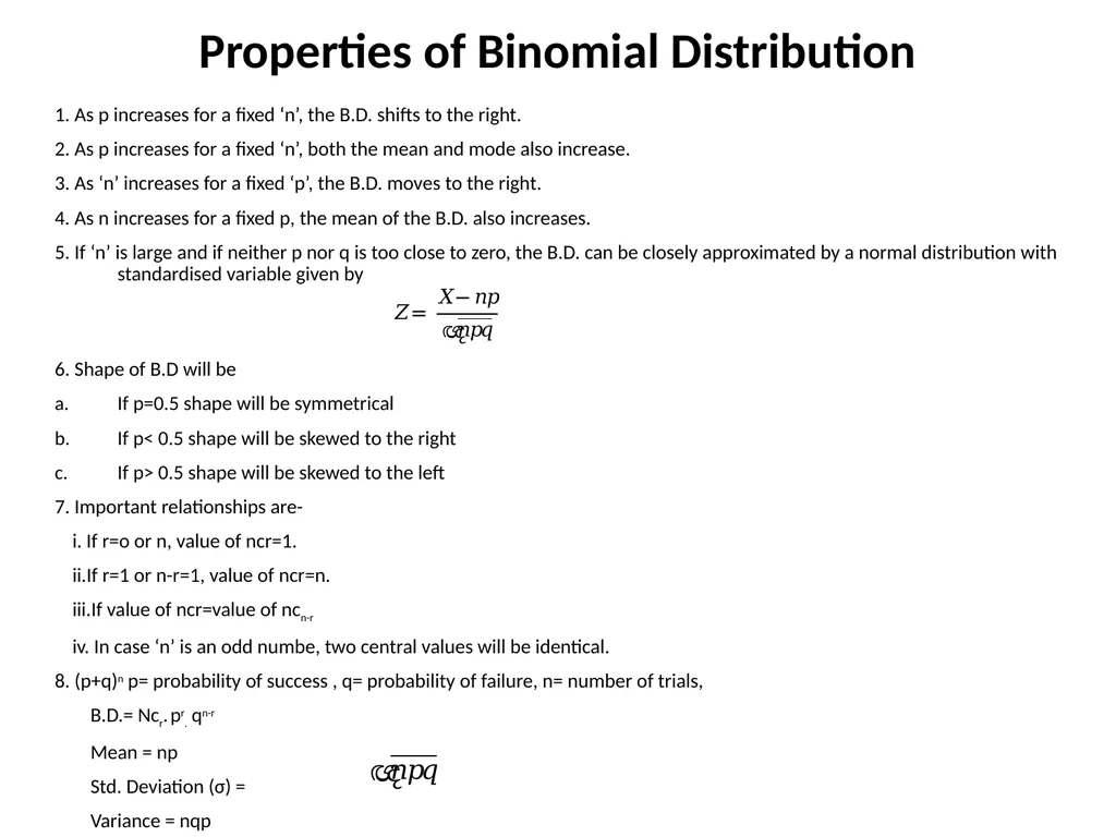
Properties of Binomial Distribution 1. As p increases for a fixed ‘n’, the B.D. shifts to the right.
2. As p increases for a fixed ‘n’, both the mean and mode also increase.
3. As ‘n’ increases for a fixed ‘p’, the B.D. moves to the right.
4. As n increases for a fixed p, the mean of the B.D. also increases.
5. If ‘n’ is large and if neither p nor q is too close to zero, the B.D. can be closely approximated by a normal distribution with standardised variable given by
6. Shape of B.D will be
If p=0.5 shape will be symmetrical
If p< 0.5 shape will be skewed to the right
If p> 0.5 shape will be skewed to the left
7. Important relationships are-
i. If r=o or n, value of ncr=1.
ii.If r=1 or n-r=1, value of ncr=n.
iii.If value of ncr=value of ncn-r
iv. In case ‘n’ is an odd numbe, two central values will be identical.
8. (p+q)n p= probability of success , q= probability of failure, n= number of trials,
B.D.= Ncr. pr. qn-r
Mean = np
Std. Deviation (σ) =
Variance = nqp<br>
08
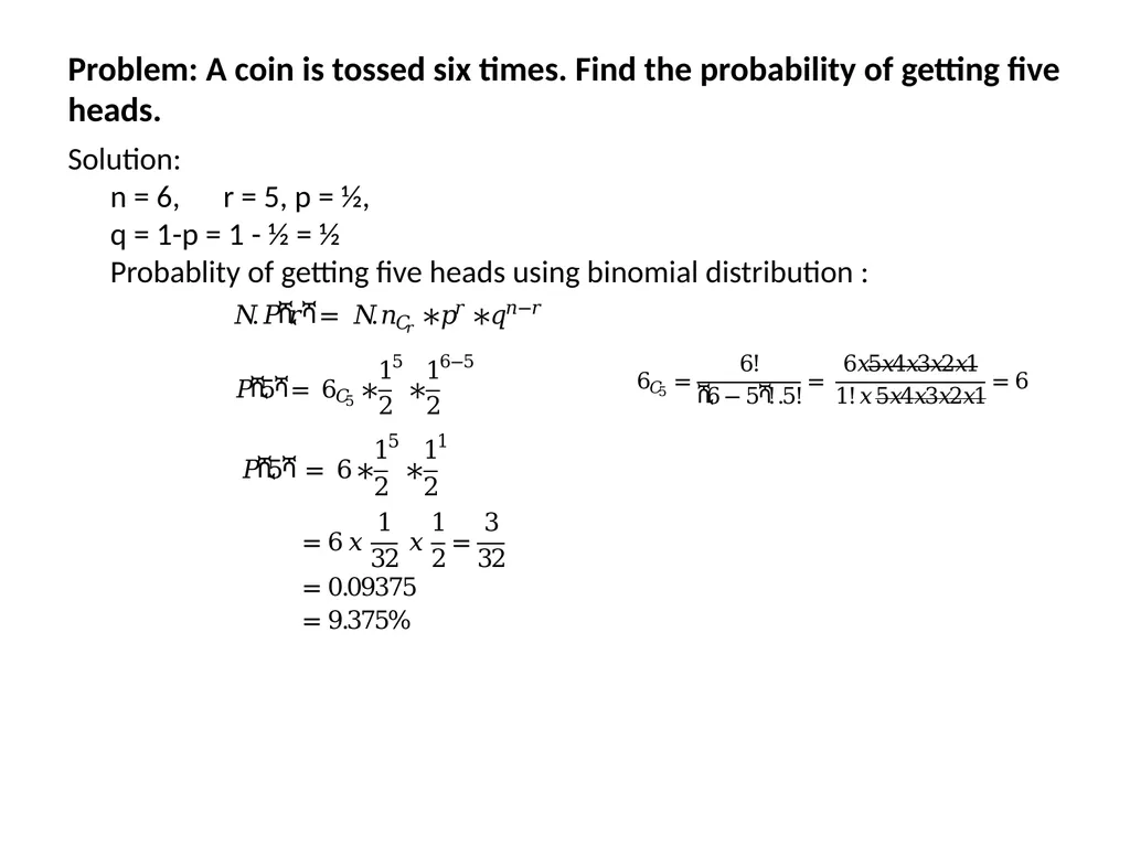
Problem: A coin is tossed six times. Find the probability of getting five heads. Solution: n = 6, r = 5, p = ½, q = 1-p = 1 - ½ = ½ Probablity of getting five heads using binomial distribution :<br>
09
Poisson Distribution In case of binomial distribution, if the exact value of ‘n’ is not known and p is very small, then it is not possible to find out binomial probabilities. Even if ‘n’ is known and it is a very large number, calculations involved will be tedious.
French Mathematician Simeon Denis Poisson (1781—1840), in1837 derived a limiting form of binomial distribution which is called as Poisson distribution.
Poisson distribution follow most of temporal and spatial distribution.<br>
10
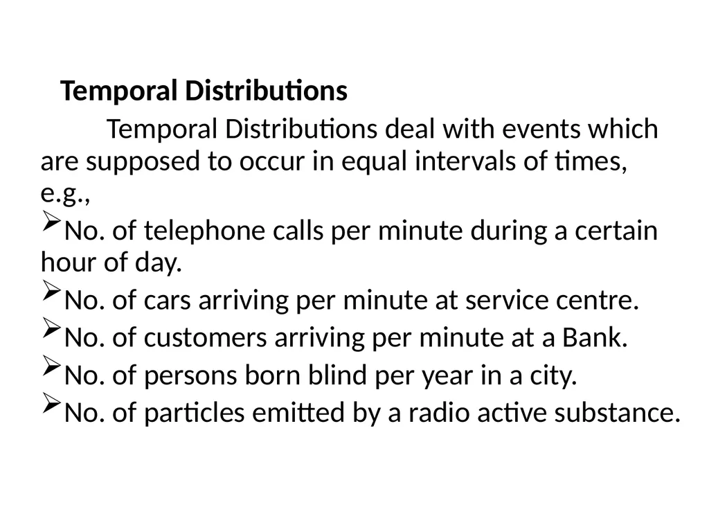
Temporal Distributions Temporal Distributions deal with events which are supposed to occur in equal intervals of times, e.g.,
No. of telephone calls per minute during a certain hour of day.
No. of cars arriving per minute at service centre.
No. of customers arriving per minute at a Bank.
No. of persons born blind per year in a city.
No. of particles emitted by a radio active substance.<br>
11
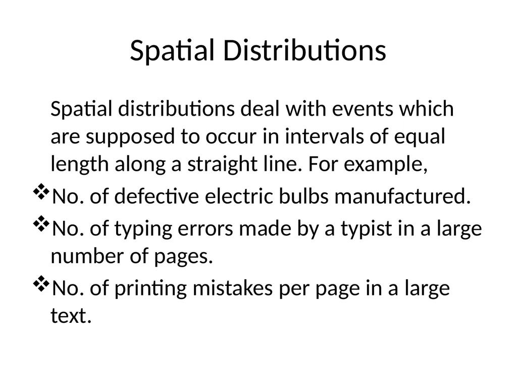
Spatial Distributions Spatial distributions deal with events which are supposed to occur in intervals of equal length along a straight line. For example,
No. of defective electric bulbs manufactured.
No. of typing errors made by a typist in a large number of pages.
No. of printing mistakes per page in a large text.<br>
12
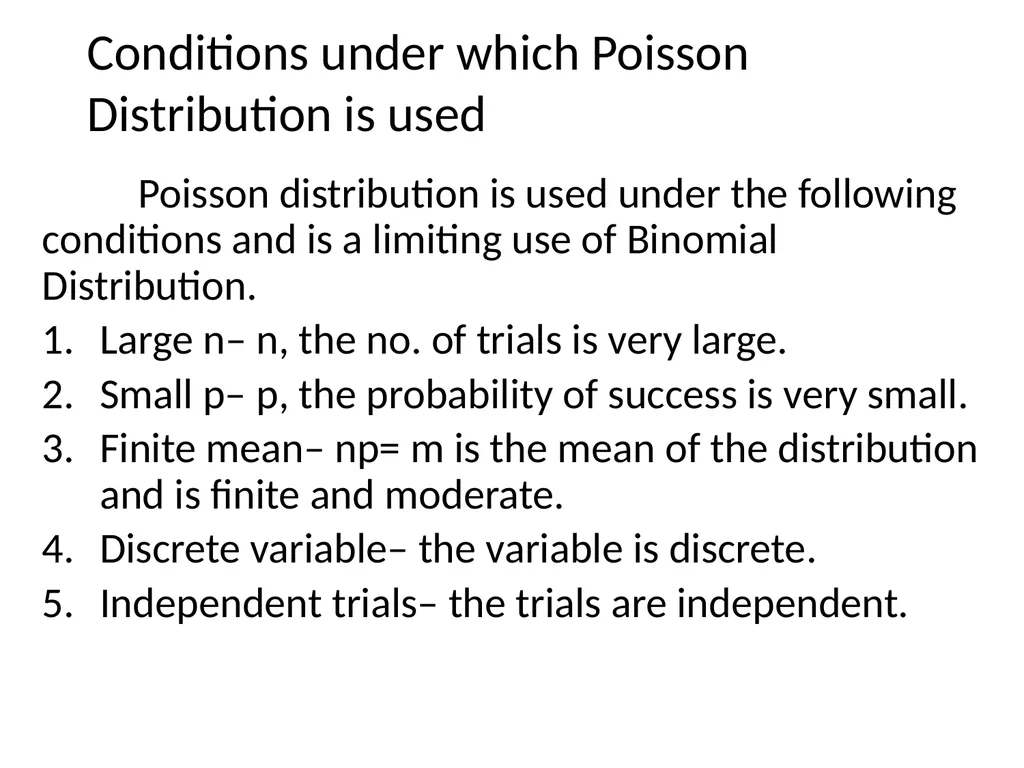
Conditions under which Poisson Distribution is used Poisson distribution is used under the following conditions and is a limiting use of Binomial Distribution.
Large n– n, the no. of trials is very large.
Small p– p, the probability of success is very small.
Finite mean– np= m is the mean of the distribution and is finite and moderate.
Discrete variable– the variable is discrete.
Independent trials– the trials are independent.<br>
13
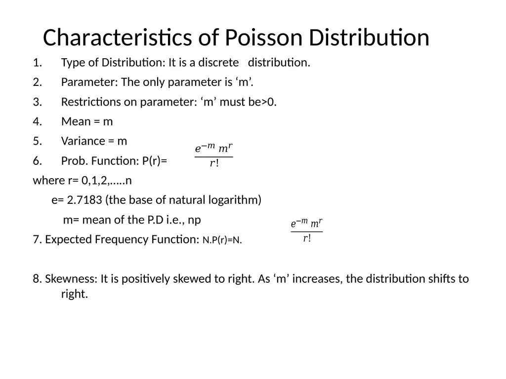
Characteristics of Poisson Distribution Type of Distribution: It is a discrete distribution.
Parameter: The only parameter is ‘m’.
Restrictions on parameter: ‘m’ must be>0.
Mean = m
Variance = m
Prob. Function: P(r)=
where r= 0,1,2,…..n
e= 2.7183 (the base of natural logarithm)
m= mean of the P.D i.e., np
7. Expected Frequency Function: N.P(r)=N.
8. Skewness: It is positively skewed to right. As ‘m’ increases, the distribution shifts to right.<br>
14
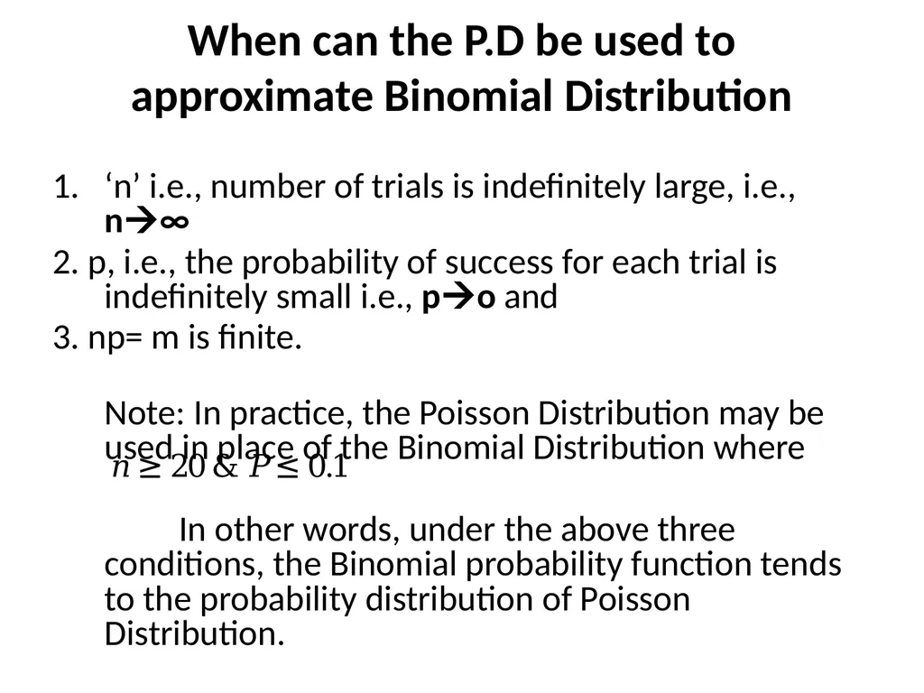
When can the P.D be used to approximate Binomial Distribution ‘n’ i.e., number of trials is indefinitely large, i.e., n∞
2. p, i.e., the probability of success for each trial is indefinitely small i.e., po and
3. np= m is finite.
Note: In practice, the Poisson Distribution may be used in place of the Binomial Distribution where
In other words, under the above three conditions, the Binomial probability function tends to the probability distribution of Poisson Distribution.<br>