
Traffic theory and congestion Traffic examples
SB
Published · 26 slides · 0 views

1 / 1



Description
Traffic theory and congestion Traffic examples Vietnam, India, Egitto, Los Angeles, Napoli, Milano, Amsterdam Goals with traffic Understanding, modelling Forecasting Governing What is a good traffic level? No congestion? Maximum speed?
Related Topics
Share
Embed code
Download this presentation From Below
"Traffic theory and congestion Traffic examples" is the property of its rightful owner. Permission is granted to download and print the materials on this website for personal, non-commercial use only, and to display it on your personal computer provided you do not modify the materials and that you retain all copyright notices contained in the materials. By downloading content from our website, you accept the terms of this agreement.
Presentation Transcript
01
Traffic theory and congestion<br>
02
Traffic examples Vietnam, India, Egitto, Los Angeles, Napoli, Milano, Amsterdam
Goals with traffic
Understanding, modelling
Forecasting
Governing<br>
Goals with traffic
Understanding, modelling
Forecasting
Governing<br>
03
What is a good traffic level? No congestion?
Maximum speed?
Maximum flow?
Optimal flow?
Private vs social point of view<br>
Maximum speed?
Maximum flow?
Optimal flow?
Private vs social point of view<br>
04
Traffic flow theory Traffic flow theory studies the interaction between vehicles, drivers, and infrastructure with the aim of
understanding and modelling traffic flows
designing an optimal road network
designing efficient traffic regulation
Nonetheless, even with the advent of significant computer processing power, to date there is no satisfactory general traffic model. Current traffic models use a mixture of empirical and theoretical techniques. These models are then used for traffic forecasts and traffic management.<br>
understanding and modelling traffic flows
designing an optimal road network
designing efficient traffic regulation
Nonetheless, even with the advent of significant computer processing power, to date there is no satisfactory general traffic model. Current traffic models use a mixture of empirical and theoretical techniques. These models are then used for traffic forecasts and traffic management.<br>
05
Different approaches between transport engineers and economists Transport engineers’ approach: observe, model, regulate traffic flows via road network planning, road space allocation, traffic lights (positioning and timing), roundabouts, one-way streets, reserved lanes (for cycling and buses), parking, public transport lines, etc..
Transport economists’ approach: take into account the localization of the economic activities, the urban form and the individuals’ and firms’ preferences. Study behaviour and analyse the impact of financial policies (vehicle purchasing price, fuel costs, ticket costs, parking fares, rents, etc.)<br>
Transport economists’ approach: take into account the localization of the economic activities, the urban form and the individuals’ and firms’ preferences. Study behaviour and analyse the impact of financial policies (vehicle purchasing price, fuel costs, ticket costs, parking fares, rents, etc.)<br>
06
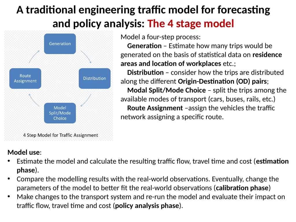
A traditional engineering traffic model for forecasting and policy analysis: The 4 stage model Model a four-step process:
Generation – Estimate how many trips would be generated on the basis of statistical data on residence areas and location of workplaces etc.;
Distribution – consider how the trips are distributed along the different Origin-Destination (OD) pairs;
Modal Split/Mode Choice – split the trips among the available modes of transport (cars, buses, rails, etc.)
Route Assignment –assign the vehicles the traffic network assigning a specific route. Model use:
Estimate the model and calculate the resulting traffic flow, travel time and cost (estimation phase).
Compare the modelling results with the real-world observations. Eventually, change the parameters of the model to better fit the real-world observations (calibration phase)
Make changes to the transport system and re-run the model and evaluate their impact on traffic flow, travel time and cost (policy analysis phase).<br>
Generation – Estimate how many trips would be generated on the basis of statistical data on residence areas and location of workplaces etc.;
Distribution – consider how the trips are distributed along the different Origin-Destination (OD) pairs;
Modal Split/Mode Choice – split the trips among the available modes of transport (cars, buses, rails, etc.)
Route Assignment –assign the vehicles the traffic network assigning a specific route. Model use:
Estimate the model and calculate the resulting traffic flow, travel time and cost (estimation phase).
Compare the modelling results with the real-world observations. Eventually, change the parameters of the model to better fit the real-world observations (calibration phase)
Make changes to the transport system and re-run the model and evaluate their impact on traffic flow, travel time and cost (policy analysis phase).<br>
07
Fundamental diagram of traffic flow<br>
08
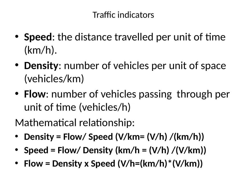
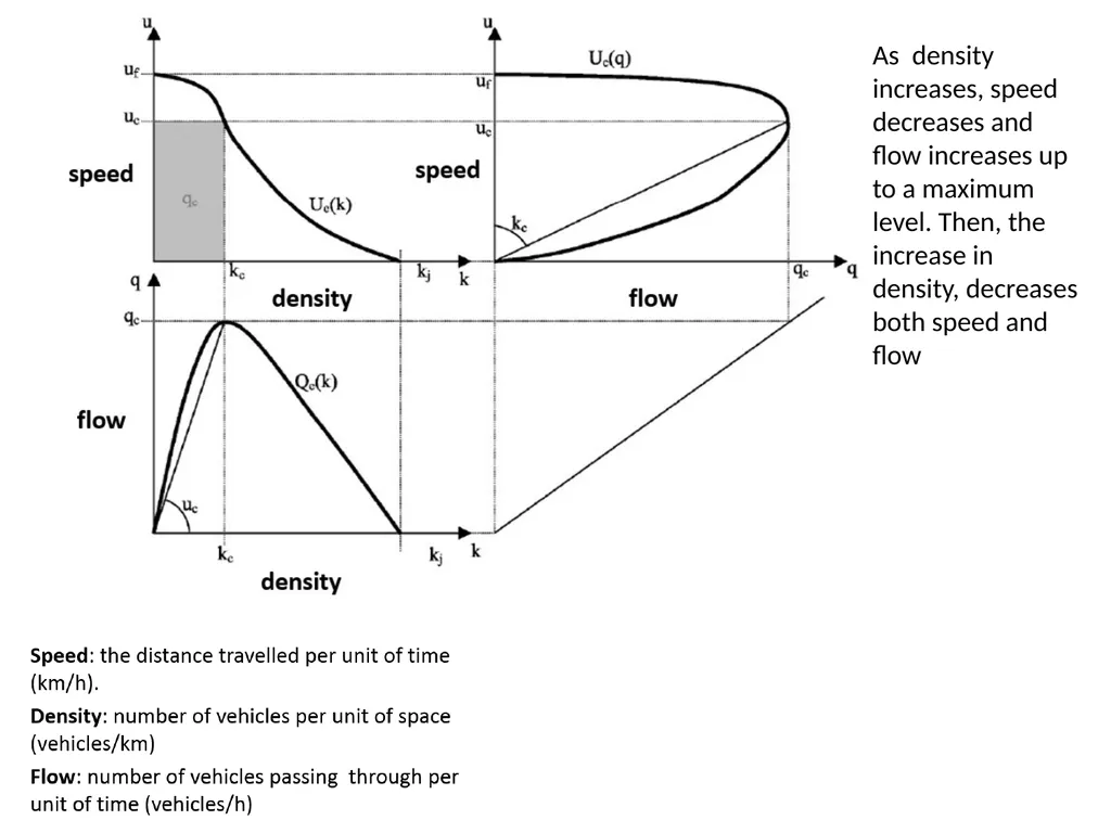
Traffic indicators Speed: the distance travelled per unit of time (km/h).
Density: number of vehicles per unit of space (vehicles/km)
Flow: number of vehicles passing through per unit of time (vehicles/h)
Mathematical relationship:
Density = Flow/ Speed (V/km= (V/h) /(km/h))
Speed = Flow/ Density (km/h = (V/h) /(V/km))
Flow = Density x Speed (V/h=(km/h)*(V/km))<br>
Density: number of vehicles per unit of space (vehicles/km)
Flow: number of vehicles passing through per unit of time (vehicles/h)
Mathematical relationship:
Density = Flow/ Speed (V/km= (V/h) /(km/h))
Speed = Flow/ Density (km/h = (V/h) /(V/km))
Flow = Density x Speed (V/h=(km/h)*(V/km))<br>
09
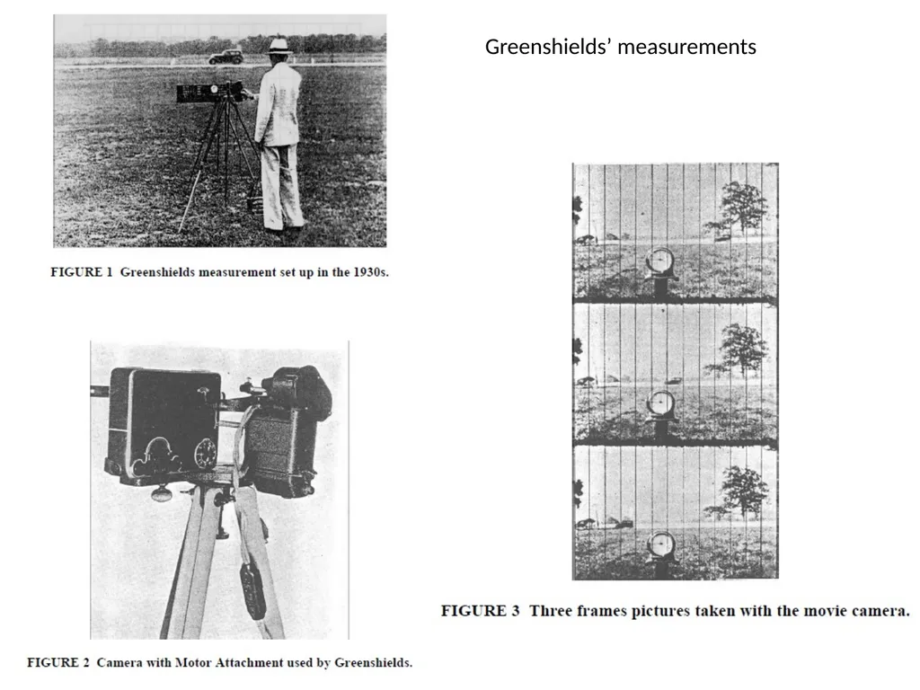
Greenshields’ measurements<br>
10
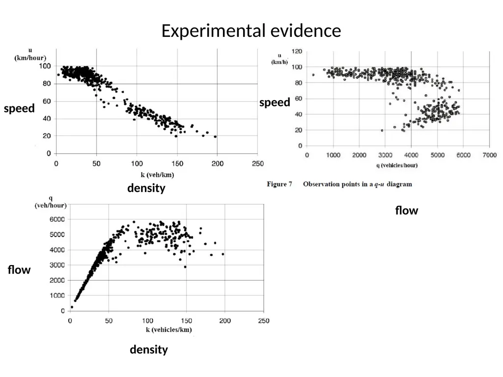
density speed flow Experimental evidence flow speed density<br>
11
As density increases, speed decreases and flow increases up to a maximum level. Then, the increase in density, decreases both speed and flow<br>
12
Greenshield’s fundamental diagram: linearized form speed density density speed flow flow<br>
13
Concepts of transport equilibria In 1952, Wardrop (John Glen Wardrop (1886–1969) was an English transport analyst) stated two principles that formalize this notion of equilibrium: the user’s optimum and the systems’ optimum<br>
14
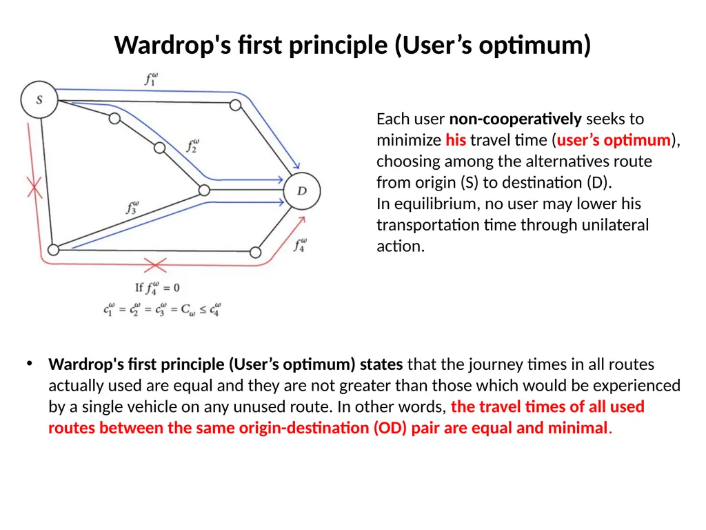
Wardrop's first principle (User’s optimum) Wardrop's first principle (User’s optimum) states that the journey times in all routes actually used are equal and they are not greater than those which would be experienced by a single vehicle on any unused route. In other words, the travel times of all used routes between the same origin-destination (OD) pair are equal and minimal. Each user non-cooperatively seeks to minimize his travel time (user’s optimum), choosing among the alternatives route from origin (S) to destination (D).
In equilibrium, no user may lower his transportation time through unilateral action.<br>
In equilibrium, no user may lower his transportation time through unilateral action.<br>
15
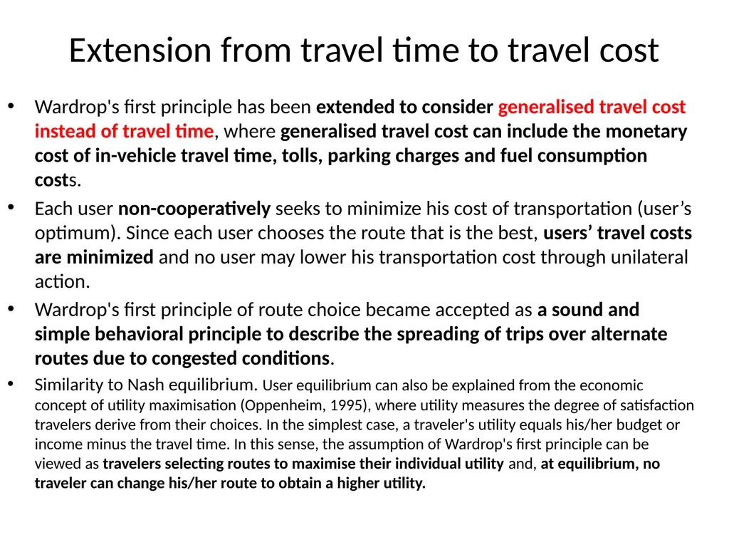
Extension from travel time to travel cost Wardrop's first principle has been extended to consider generalised travel cost instead of travel time, where generalised travel cost can include the monetary cost of in-vehicle travel time, tolls, parking charges and fuel consumption costs.
Each user non-cooperatively seeks to minimize his cost of transportation (user’s optimum). Since each user chooses the route that is the best, users’ travel costs are minimized and no user may lower his transportation cost through unilateral action.
Wardrop's first principle of route choice became accepted as a sound and simple behavioral principle to describe the spreading of trips over alternate routes due to congested conditions.
Similarity to Nash equilibrium. User equilibrium can also be explained from the economic concept of utility maximisation (Oppenheim, 1995), where utility measures the degree of satisfaction travelers derive from their choices. In the simplest case, a traveler's utility equals his/her budget or income minus the travel time. In this sense, the assumption of Wardrop's first principle can be viewed as travelers selecting routes to maximise their individual utility and, at equilibrium, no traveler can change his/her route to obtain a higher utility.<br>
Each user non-cooperatively seeks to minimize his cost of transportation (user’s optimum). Since each user chooses the route that is the best, users’ travel costs are minimized and no user may lower his transportation cost through unilateral action.
Wardrop's first principle of route choice became accepted as a sound and simple behavioral principle to describe the spreading of trips over alternate routes due to congested conditions.
Similarity to Nash equilibrium. User equilibrium can also be explained from the economic concept of utility maximisation (Oppenheim, 1995), where utility measures the degree of satisfaction travelers derive from their choices. In the simplest case, a traveler's utility equals his/her budget or income minus the travel time. In this sense, the assumption of Wardrop's first principle can be viewed as travelers selecting routes to maximise their individual utility and, at equilibrium, no traveler can change his/her route to obtain a higher utility.<br>
16
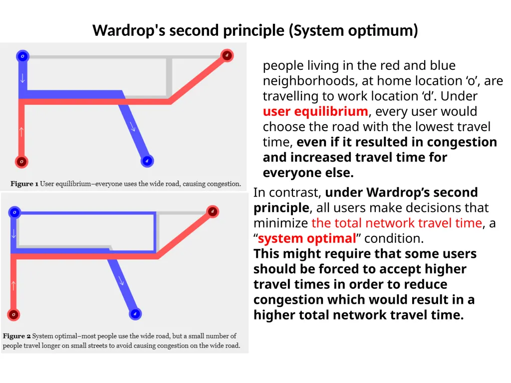
Wardrop's second principle (System optimum) people living in the red and blue neighborhoods, at home location ‘o’, are travelling to work location ‘d’. Under user equilibrium, every user would choose the road with the lowest travel time, even if it resulted in congestion and increased travel time for everyone else. In contrast, under Wardrop’s second principle, all users make decisions that minimize the total network travel time, a “system optimal” condition.
This might require that some users should be forced to accept higher travel times in order to reduce congestion which would result in a higher total network travel time.<br>
This might require that some users should be forced to accept higher travel times in order to reduce congestion which would result in a higher total network travel time.<br>
17
Wardrop's second principle (System optimum) states: At System optimal equilibrium the total travel time is at the minimum. The two equilibria might differ.
How to reach system optimum?
Quantitative regulations: right of the way, access restriction, reserved lanes, one-way streets, traffic lights, parking restrictions, speed limits
Economic incentives: congestion charge, vehicle tax, fuel tax
Economists argue in favor of marginal cost road pricing (minimum social costs) via a congestion charge.
Sometimes, these measures can be very political and wildly unpopular.<br>
How to reach system optimum?
Quantitative regulations: right of the way, access restriction, reserved lanes, one-way streets, traffic lights, parking restrictions, speed limits
Economic incentives: congestion charge, vehicle tax, fuel tax
Economists argue in favor of marginal cost road pricing (minimum social costs) via a congestion charge.
Sometimes, these measures can be very political and wildly unpopular.<br>
18
Congestion pricing to achieve the social optimum<br>
19
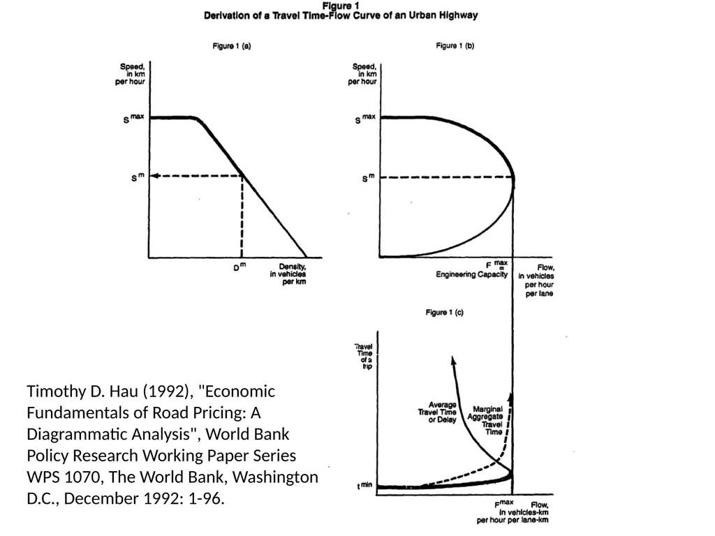
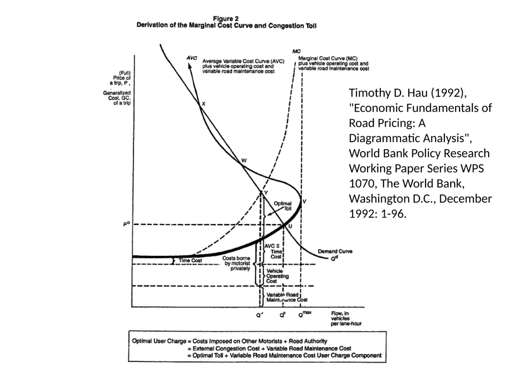
Timothy D. Hau (1992), "Economic Fundamentals of Road Pricing: A Diagrammatic Analysis", World Bank Policy Research Working Paper Series WPS 1070, The World Bank, Washington D.C., December 1992: 1-96.<br>
20
Timothy D. Hau (1992), "Economic Fundamentals of Road Pricing: A Diagrammatic Analysis", World Bank Policy Research Working Paper Series WPS 1070, The World Bank, Washington D.C., December 1992: 1-96.<br>
21
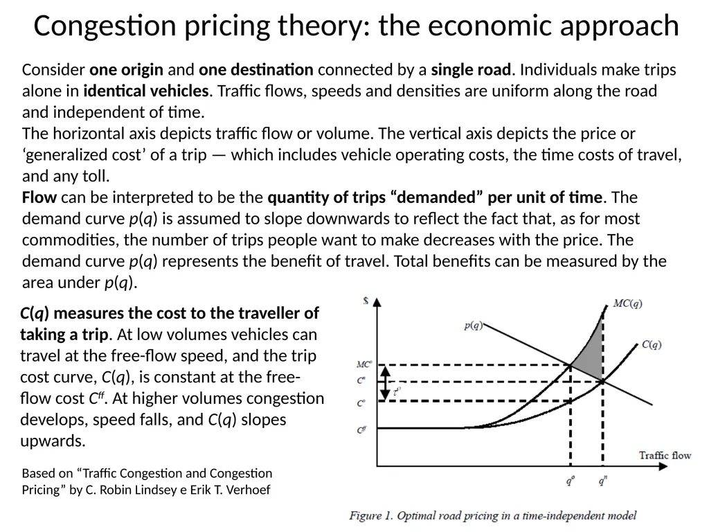
Consider one origin and one destination connected by a single road. Individuals make trips alone in identical vehicles. Traffic flows, speeds and densities are uniform along the road and independent of time.
The horizontal axis depicts traffic flow or volume. The vertical axis depicts the price or ‘generalized cost’ of a trip — which includes vehicle operating costs, the time costs of travel, and any toll.
Flow can be interpreted to be the quantity of trips “demanded” per unit of time. The demand curve p(q) is assumed to slope downwards to reflect the fact that, as for most commodities, the number of trips people want to make decreases with the price. The demand curve p(q) represents the benefit of travel. Total benefits can be measured by the area under p(q). Congestion pricing theory: the economic approach Based on “Traffic Congestion and Congestion Pricing” by C. Robin Lindsey e Erik T. Verhoef C(q) measures the cost to the traveller of taking a trip. At low volumes vehicles can travel at the free-flow speed, and the trip cost curve, C(q), is constant at the free- flow cost Cff. At higher volumes congestion develops, speed falls, and C(q) slopes upwards.<br>
The horizontal axis depicts traffic flow or volume. The vertical axis depicts the price or ‘generalized cost’ of a trip — which includes vehicle operating costs, the time costs of travel, and any toll.
Flow can be interpreted to be the quantity of trips “demanded” per unit of time. The demand curve p(q) is assumed to slope downwards to reflect the fact that, as for most commodities, the number of trips people want to make decreases with the price. The demand curve p(q) represents the benefit of travel. Total benefits can be measured by the area under p(q). Congestion pricing theory: the economic approach Based on “Traffic Congestion and Congestion Pricing” by C. Robin Lindsey e Erik T. Verhoef C(q) measures the cost to the traveller of taking a trip. At low volumes vehicles can travel at the free-flow speed, and the trip cost curve, C(q), is constant at the free- flow cost Cff. At higher volumes congestion develops, speed falls, and C(q) slopes upwards.<br>
22
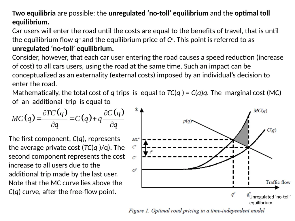
Two equilibria are possible: the unregulated ‘no-toll’ equilibrium and the optimal toll equilibrium.
Car users will enter the road until the costs are equal to the benefits of travel, that is until the equilibrium flow qn and the equilibrium price of Cn. This point is referred to as unregulated ‘no-toll’ equilibrium.
Consider, however, that each car user entering the road causes a speed reduction (increase of cost) to all cars users, using the road at the same time. Such an impact can be conceptualized as an externality (external costs) imposed by an individual’s decision to enter the road.
Mathematically, the total cost of q trips is equal to TC(q ) = C(q)q. The marginal cost (MC) of an additional trip is equal to Unregulated ‘no-toll’ equilibrium The first component, C(q), represents the average private cost (TC(q )/q). The second component represents the cost increase to all users due to the additional trip made by the last user.
Note that the MC curve lies above the C(q) curve, after the free-flow point.<br>
Car users will enter the road until the costs are equal to the benefits of travel, that is until the equilibrium flow qn and the equilibrium price of Cn. This point is referred to as unregulated ‘no-toll’ equilibrium.
Consider, however, that each car user entering the road causes a speed reduction (increase of cost) to all cars users, using the road at the same time. Such an impact can be conceptualized as an externality (external costs) imposed by an individual’s decision to enter the road.
Mathematically, the total cost of q trips is equal to TC(q ) = C(q)q. The marginal cost (MC) of an additional trip is equal to Unregulated ‘no-toll’ equilibrium The first component, C(q), represents the average private cost (TC(q )/q). The second component represents the cost increase to all users due to the additional trip made by the last user.
Note that the MC curve lies above the C(q) curve, after the free-flow point.<br>
23
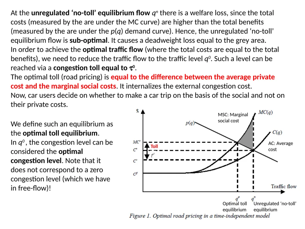
At the unregulated ‘no-toll’ equilibrium flow qn there is a welfare loss, since the total costs (measured by the are under the MC curve) are higher than the total benefits (measured by the are under the p(q) demand curve). Hence, the unregulated ‘no-toll’ equilibrium flow is sub-optimal. It causes a deadweight loss equal to the grey area.
In order to achieve the optimal traffic flow (where the total costs are equal to the total benefits), we need to reduce the traffic flow to the traffic level q0. Such a level can be reached via a congestion toll equal to t0.
The optimal toll (road pricing) is equal to the difference between the average private cost and the marginal social costs. It internalizes the external congestion cost.
Now, car users decide on whether to make a car trip on the basis of the social and not on their private costs. AC: Average cost MSC: Marginal social cost Unregulated ‘no-toll’ equilibrium Optimal toll equilibrium We define such an equilibrium as the optimal toll equilibrium.
In q0 , the congestion level can be considered the optimal congestion level. Note that it does not correspond to a zero congestion level (which we have in free-flow)! Toll<br>
In order to achieve the optimal traffic flow (where the total costs are equal to the total benefits), we need to reduce the traffic flow to the traffic level q0. Such a level can be reached via a congestion toll equal to t0.
The optimal toll (road pricing) is equal to the difference between the average private cost and the marginal social costs. It internalizes the external congestion cost.
Now, car users decide on whether to make a car trip on the basis of the social and not on their private costs. AC: Average cost MSC: Marginal social cost Unregulated ‘no-toll’ equilibrium Optimal toll equilibrium We define such an equilibrium as the optimal toll equilibrium.
In q0 , the congestion level can be considered the optimal congestion level. Note that it does not correspond to a zero congestion level (which we have in free-flow)! Toll<br>
24
Road pricing or congestion pricing The use of toll to achieve a system optimum, the optimal congestion level, is known as road pricing or congestion pricing.
The system optimum is achieved via a financial incentives instead of via regulation or physical measures . Toll<br>
The system optimum is achieved via a financial incentives instead of via regulation or physical measures . Toll<br>
25
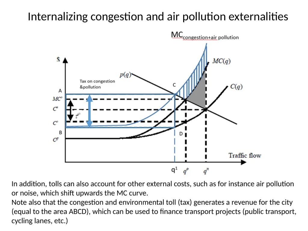
Internalizing congestion and air pollution externalities In addition, tolls can also account for other external costs, such as for instance air pollution or noise, which shift upwards the MC curve.
Note also that the congestion and environmental toll (tax) generates a revenue for the city (equal to the area ABCD), which can be used to finance transport projects (public transport, cycling lanes, etc.)<br>
Note also that the congestion and environmental toll (tax) generates a revenue for the city (equal to the area ABCD), which can be used to finance transport projects (public transport, cycling lanes, etc.)<br>
26
Ecopass, Area C and Area B: implemented policy to reduce congestion and air pollution in Milan<br>