
Tutorial lecture Basics of Spinach with optimal
OM
Published · 20 slides · 0 views
1 / 1
Description
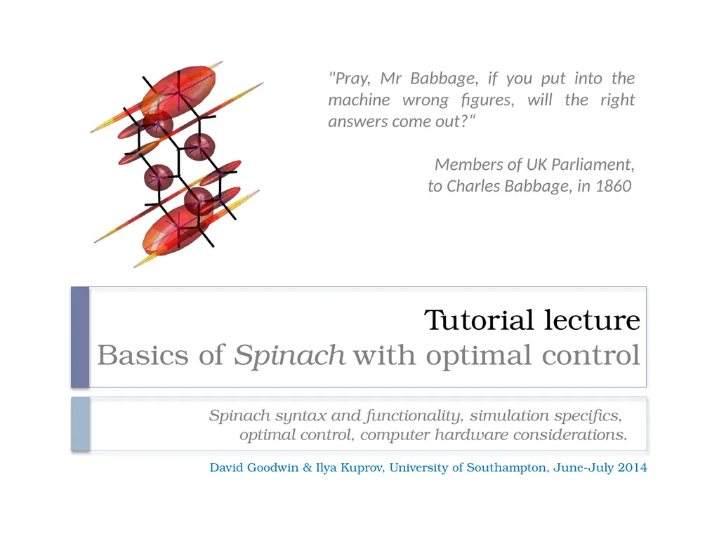
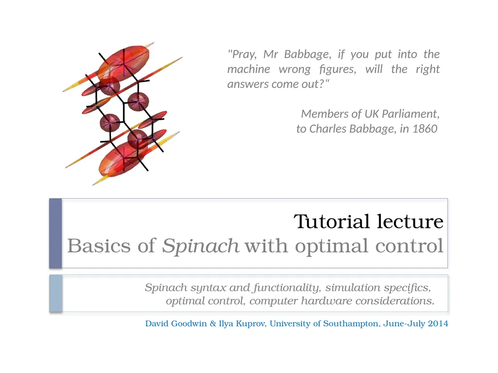
Tutorial lecture Basics of Spinach with optimal control Spinach syntax and functionality, simulation specifics, optimal control, computer hardware considerations. David Goodwin Ilya Kuprov, University of Southampton, June-July 2014 Pray,
Related Topics
Share
Embed code
Download this presentation From Below
"Tutorial lecture Basics of Spinach with optimal" is the property of its rightful owner. Permission is granted to download and print the materials on this website for personal, non-commercial use only, and to display it on your personal computer provided you do not modify the materials and that you retain all copyright notices contained in the materials. By downloading content from our website, you accept the terms of this agreement.
Presentation Transcript
01
Tutorial lecture
Basics of Spinach with optimal control Spinach syntax and functionality, simulation specifics,
optimal control, computer hardware considerations. David Goodwin & Ilya Kuprov, University of Southampton, June-July 2014 "Pray, Mr Babbage, if you put into the machine wrong figures, will the right answers come out?“
Members of UK Parliament,
to Charles Babbage, in 1860<br>
Members of UK Parliament,
to Charles Babbage, in 1860<br>
02
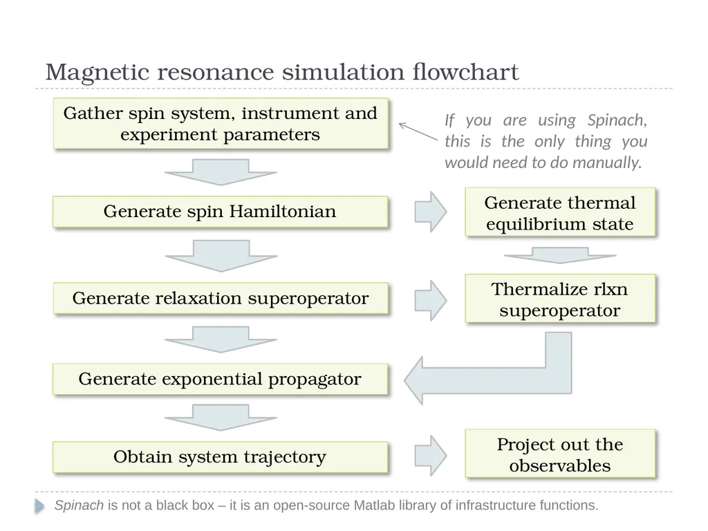
Magnetic resonance simulation flowchart Spinach is not a black box – it is an open-source Matlab library of infrastructure functions. Gather spin system, instrument and experiment parameters Generate spin Hamiltonian Generate relaxation superoperator Generate thermal equilibrium state Thermalize rlxn superoperator Generate exponential propagator If you are using Spinach, this is the only thing you would need to do manually. Obtain system trajectory Project out the observables<br>
03
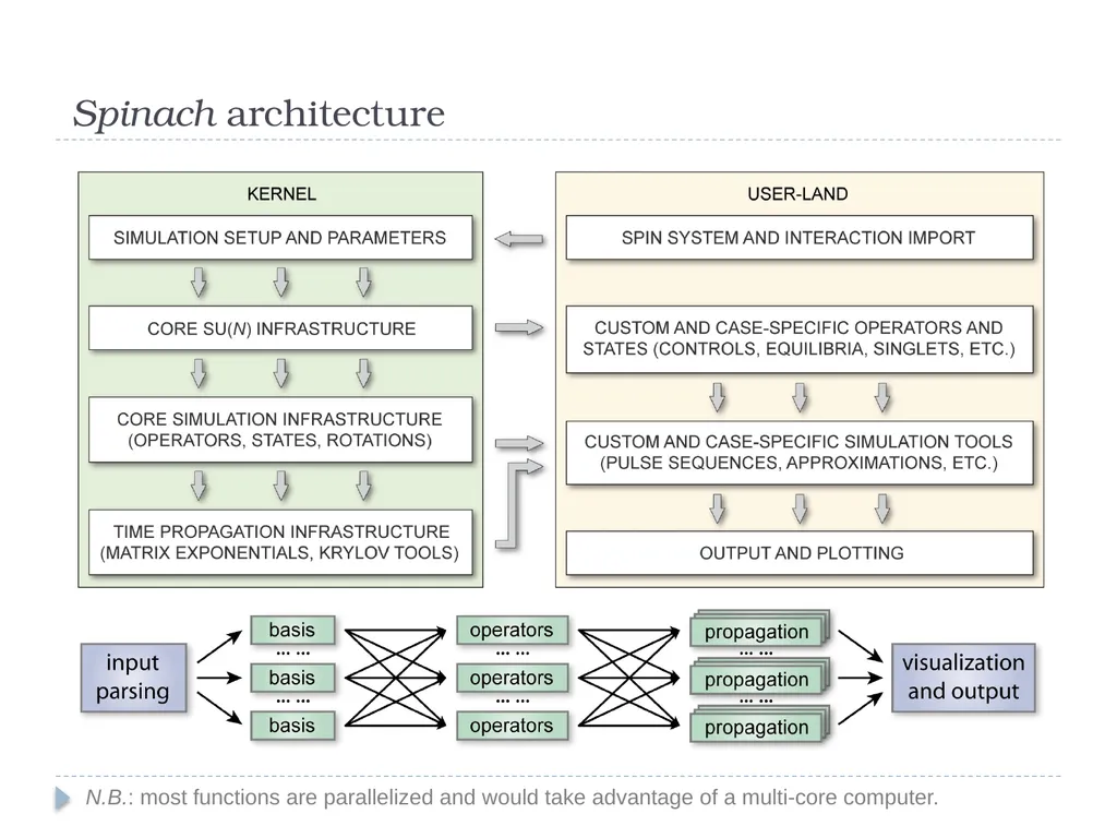
Spinach architecture N.B.: most functions are parallelized and would take advantage of a multi-core computer.<br>
04
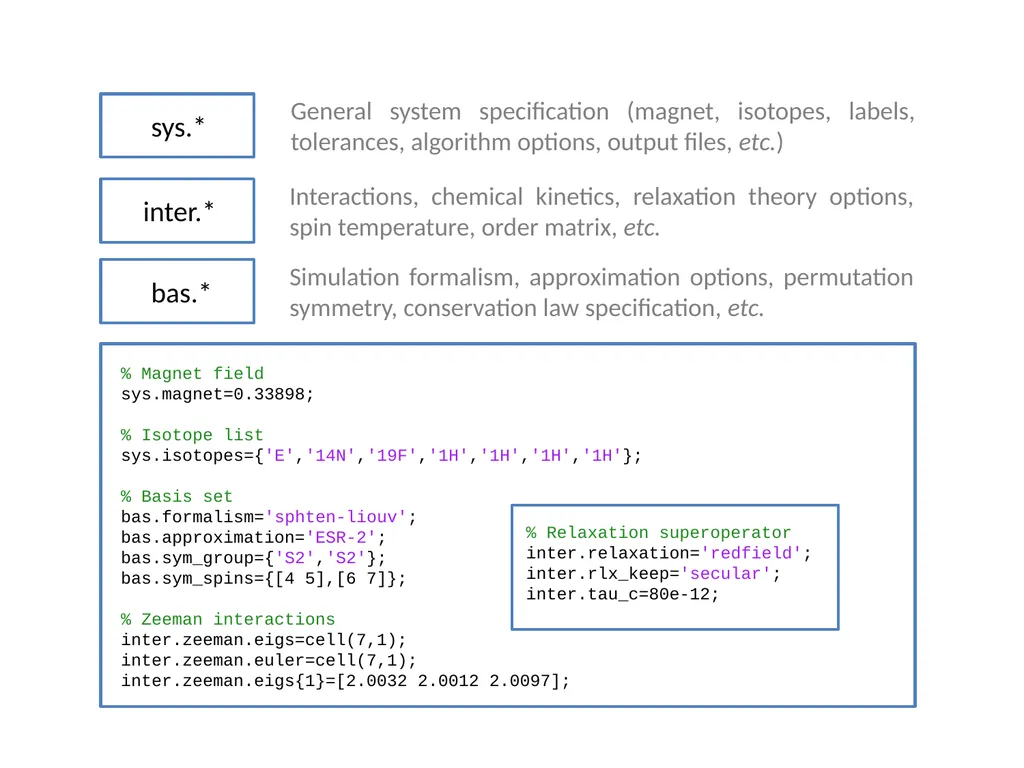
sys.* inter.* bas.* General system specification (magnet, isotopes, labels, tolerances, algorithm options, output files, etc.) Interactions, chemical kinetics, relaxation theory options, spin temperature, order matrix, etc. Simulation formalism, approximation options, permutation symmetry, conservation law specification, etc. % Magnet field
sys.magnet=0.33898;
% Isotope list
sys.isotopes={'E','14N','19F','1H','1H','1H','1H'};
% Basis set
bas.formalism='sphten-liouv';
bas.approximation='ESR-2';
bas.sym_group={'S2','S2'};
bas.sym_spins={[4 5],[6 7]};
% Zeeman interactions
inter.zeeman.eigs=cell(7,1);
inter.zeeman.euler=cell(7,1);
inter.zeeman.eigs{1}=[2.0032 2.0012 2.0097]; % Relaxation superoperator
inter.relaxation='redfield';
inter.rlx_keep='secular';
inter.tau_c=80e-12;<br>
sys.magnet=0.33898;
% Isotope list
sys.isotopes={'E','14N','19F','1H','1H','1H','1H'};
% Basis set
bas.formalism='sphten-liouv';
bas.approximation='ESR-2';
bas.sym_group={'S2','S2'};
bas.sym_spins={[4 5],[6 7]};
% Zeeman interactions
inter.zeeman.eigs=cell(7,1);
inter.zeeman.euler=cell(7,1);
inter.zeeman.eigs{1}=[2.0032 2.0012 2.0097]; % Relaxation superoperator
inter.relaxation='redfield';
inter.rlx_keep='secular';
inter.tau_c=80e-12;<br>
05
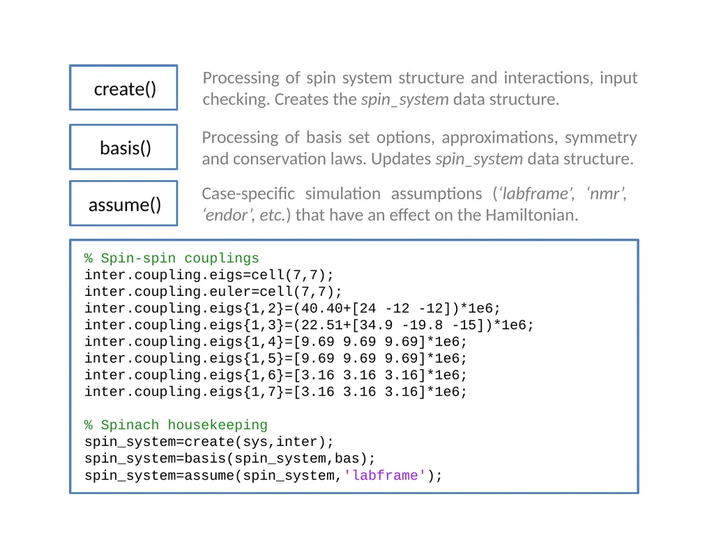
create() basis() assume() Processing of spin system structure and interactions, input checking. Creates the spin_system data structure. Processing of basis set options, approximations, symmetry and conservation laws. Updates spin_system data structure. Case-specific simulation assumptions (‘labframe’, ‘nmr’, ‘endor’, etc.) that have an effect on the Hamiltonian. % Spin-spin couplings
inter.coupling.eigs=cell(7,7);
inter.coupling.euler=cell(7,7);
inter.coupling.eigs{1,2}=(40.40+[24 -12 -12])*1e6;
inter.coupling.eigs{1,3}=(22.51+[34.9 -19.8 -15])*1e6;
inter.coupling.eigs{1,4}=[9.69 9.69 9.69]*1e6;
inter.coupling.eigs{1,5}=[9.69 9.69 9.69]*1e6;
inter.coupling.eigs{1,6}=[3.16 3.16 3.16]*1e6;
inter.coupling.eigs{1,7}=[3.16 3.16 3.16]*1e6;
% Spinach housekeeping
spin_system=create(sys,inter);
spin_system=basis(spin_system,bas);
spin_system=assume(spin_system,'labframe');<br>
inter.coupling.eigs=cell(7,7);
inter.coupling.euler=cell(7,7);
inter.coupling.eigs{1,2}=(40.40+[24 -12 -12])*1e6;
inter.coupling.eigs{1,3}=(22.51+[34.9 -19.8 -15])*1e6;
inter.coupling.eigs{1,4}=[9.69 9.69 9.69]*1e6;
inter.coupling.eigs{1,5}=[9.69 9.69 9.69]*1e6;
inter.coupling.eigs{1,6}=[3.16 3.16 3.16]*1e6;
inter.coupling.eigs{1,7}=[3.16 3.16 3.16]*1e6;
% Spinach housekeeping
spin_system=create(sys,inter);
spin_system=basis(spin_system,bas);
spin_system=assume(spin_system,'labframe');<br>
06
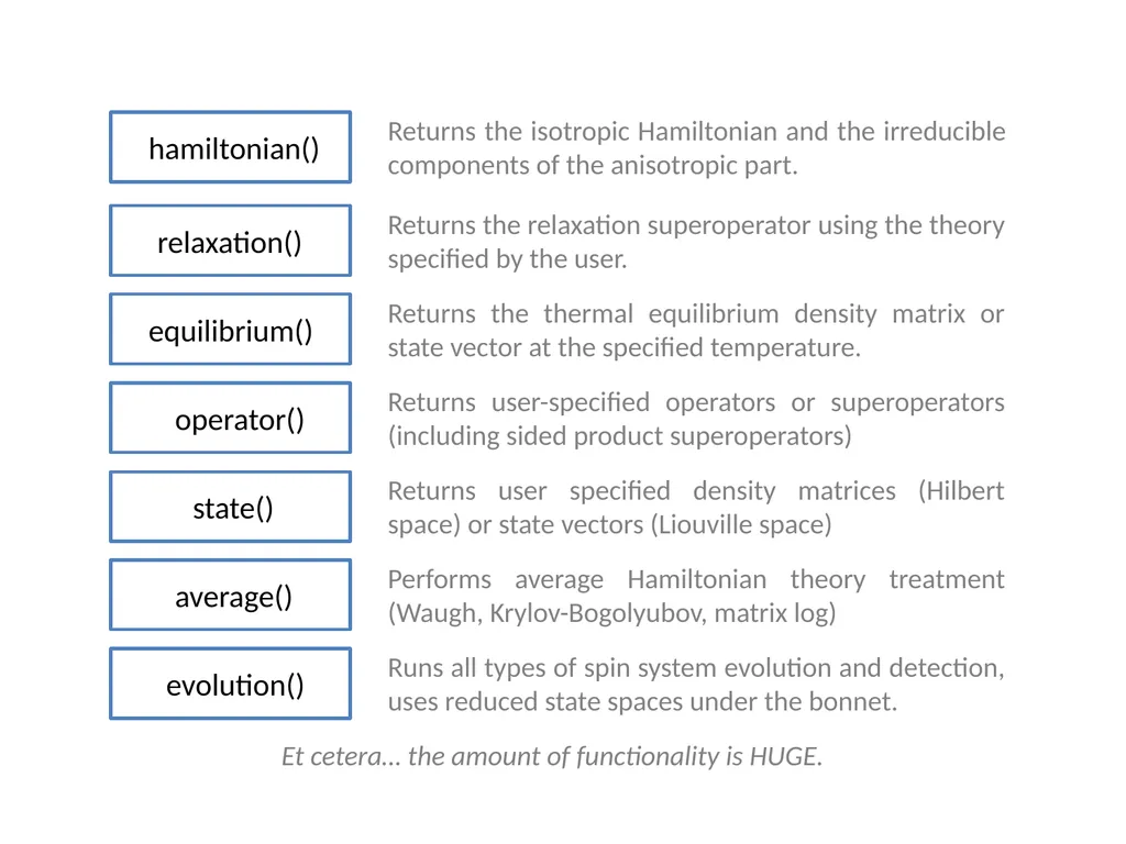
hamiltonian() relaxation() equilibrium() Returns the isotropic Hamiltonian and the irreducible components of the anisotropic part. Returns the relaxation superoperator using the theory specified by the user. Returns the thermal equilibrium density matrix or state vector at the specified temperature. operator() state() Returns user-specified operators or superoperators (including sided product superoperators) Returns user specified density matrices (Hilbert space) or state vectors (Liouville space) average() evolution() Performs average Hamiltonian theory treatment (Waugh, Krylov-Bogolyubov, matrix log) Runs all types of spin system evolution and detection, uses reduced state spaces under the bonnet. Et cetera… the amount of functionality is HUGE.<br>
07
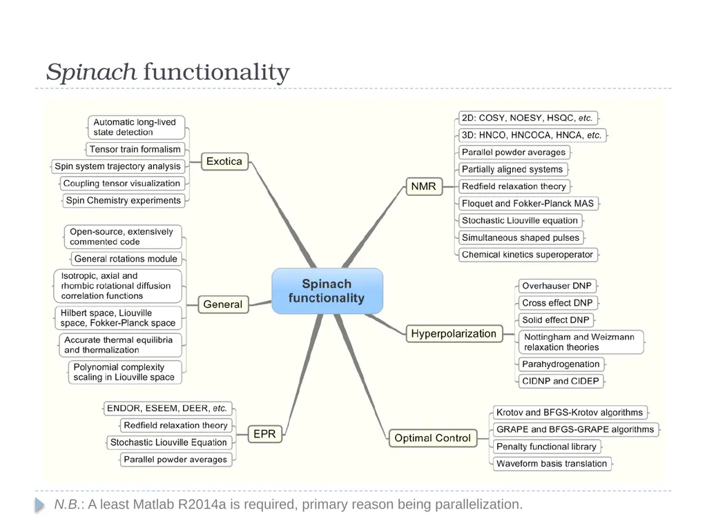
Spinach functionality N.B.: A least Matlab R2014a is required, primary reason being parallelization.<br>
08
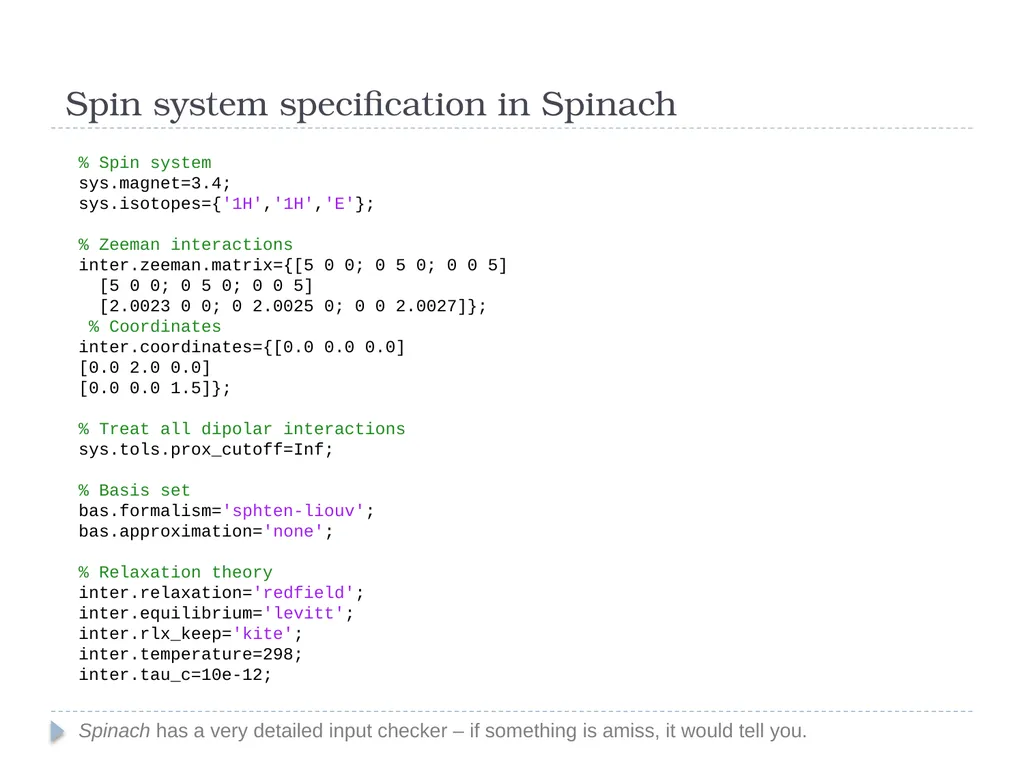
Spin system specification in Spinach Spinach has a very detailed input checker – if something is amiss, it would tell you. % Spin system
sys.magnet=3.4;
sys.isotopes={'1H','1H','E'};
% Zeeman interactions
inter.zeeman.matrix={[5 0 0; 0 5 0; 0 0 5]
[5 0 0; 0 5 0; 0 0 5]
[2.0023 0 0; 0 2.0025 0; 0 0 2.0027]};
% Coordinates
inter.coordinates={[0.0 0.0 0.0]
[0.0 2.0 0.0]
[0.0 0.0 1.5]};
% Treat all dipolar interactions
sys.tols.prox_cutoff=Inf;
% Basis set
bas.formalism='sphten-liouv';
bas.approximation='none';
% Relaxation theory
inter.relaxation='redfield';
inter.equilibrium='levitt';
inter.rlx_keep='kite';
inter.temperature=298;
inter.tau_c=10e-12;<br>
sys.magnet=3.4;
sys.isotopes={'1H','1H','E'};
% Zeeman interactions
inter.zeeman.matrix={[5 0 0; 0 5 0; 0 0 5]
[5 0 0; 0 5 0; 0 0 5]
[2.0023 0 0; 0 2.0025 0; 0 0 2.0027]};
% Coordinates
inter.coordinates={[0.0 0.0 0.0]
[0.0 2.0 0.0]
[0.0 0.0 1.5]};
% Treat all dipolar interactions
sys.tols.prox_cutoff=Inf;
% Basis set
bas.formalism='sphten-liouv';
bas.approximation='none';
% Relaxation theory
inter.relaxation='redfield';
inter.equilibrium='levitt';
inter.rlx_keep='kite';
inter.temperature=298;
inter.tau_c=10e-12;<br>
09
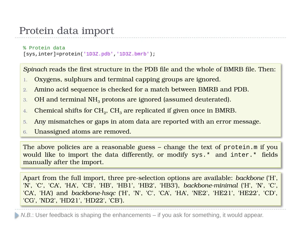
Protein data import N.B.: User feedback is shaping the enhancements – if you ask for something, it would appear. % Protein data
[sys,inter]=protein('1D3Z.pdb','1D3Z.bmrb'); Spinach reads the first structure in the PDB file and the whole of BMRB file. Then:
Oxygens, sulphurs and terminal capping groups are ignored.
Amino acid sequence is checked for a match between BMRB and PDB.
OH and terminal NH3 protons are ignored (assumed deuterated).
Chemical shifts for CH2, CH3 are replicated if given once in BMRB.
Any mismatches or gaps in atom data are reported with an error message.
Unassigned atoms are removed. The above policies are a reasonable guess – change the text of protein.m if you would like to import the data differently, or modify sys.* and inter.* fields manually after the import. Apart from the full import, three pre-selection options are available: backbone ('H', 'N', 'C', 'CA', 'HA', 'CB', 'HB', 'HB1', 'HB2', 'HB3'), backbone-minimal ('H', 'N', 'C', 'CA', 'HA') and backbone-hsqc ('H', 'N', 'C', 'CA', 'HA', 'NE2', 'HE21', 'HE22', 'CD', 'CG', 'ND2', 'HD21', 'HD22', 'CB').<br>
[sys,inter]=protein('1D3Z.pdb','1D3Z.bmrb'); Spinach reads the first structure in the PDB file and the whole of BMRB file. Then:
Oxygens, sulphurs and terminal capping groups are ignored.
Amino acid sequence is checked for a match between BMRB and PDB.
OH and terminal NH3 protons are ignored (assumed deuterated).
Chemical shifts for CH2, CH3 are replicated if given once in BMRB.
Any mismatches or gaps in atom data are reported with an error message.
Unassigned atoms are removed. The above policies are a reasonable guess – change the text of protein.m if you would like to import the data differently, or modify sys.* and inter.* fields manually after the import. Apart from the full import, three pre-selection options are available: backbone ('H', 'N', 'C', 'CA', 'HA', 'CB', 'HB', 'HB1', 'HB2', 'HB3'), backbone-minimal ('H', 'N', 'C', 'CA', 'HA') and backbone-hsqc ('H', 'N', 'C', 'CA', 'HA', 'NE2', 'HE21', 'HE22', 'CD', 'CG', 'ND2', 'HD21', 'HD22', 'CB').<br>
10
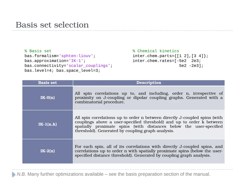
Basis set selection N.B. Many further optimizations available – see the basis preparation section of the manual. % Basis set
bas.formalism='sphten-liouv';
bas.approximation='IK-1';
bas.connectivity='scalar_couplings';
bas.level=4; bas.space_level=3; % Chemical kinetics
inter.chem.parts={[1 2],[3 4]};
inter.chem.rates=[-5e2 2e3;
5e2 -2e3];<br>
bas.formalism='sphten-liouv';
bas.approximation='IK-1';
bas.connectivity='scalar_couplings';
bas.level=4; bas.space_level=3; % Chemical kinetics
inter.chem.parts={[1 2],[3 4]};
inter.chem.rates=[-5e2 2e3;
5e2 -2e3];<br>
11
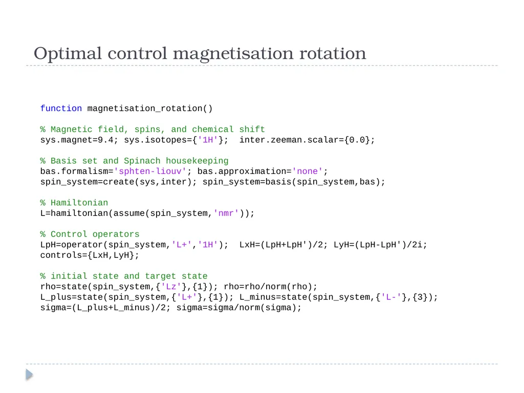
Optimal control magnetisation rotation function magnetisation_rotation()
% Magnetic field, spins, and chemical shift
sys.magnet=9.4; sys.isotopes={'1H'}; inter.zeeman.scalar={0.0};
% Basis set and Spinach housekeeping
bas.formalism='sphten-liouv'; bas.approximation='none';
spin_system=create(sys,inter); spin_system=basis(spin_system,bas);
% Hamiltonian
L=hamiltonian(assume(spin_system,'nmr'));
% Control operators
LpH=operator(spin_system,'L+','1H'); LxH=(LpH+LpH')/2; LyH=(LpH-LpH')/2i; controls={LxH,LyH};
% initial state and target state
rho=state(spin_system,{'Lz'},{1}); rho=rho/norm(rho);
L_plus=state(spin_system,{'L+'},{1}); L_minus=state(spin_system,{'L-'},{3});
sigma=(L_plus+L_minus)/2; sigma=sigma/norm(sigma);<br>
% Magnetic field, spins, and chemical shift
sys.magnet=9.4; sys.isotopes={'1H'}; inter.zeeman.scalar={0.0};
% Basis set and Spinach housekeeping
bas.formalism='sphten-liouv'; bas.approximation='none';
spin_system=create(sys,inter); spin_system=basis(spin_system,bas);
% Hamiltonian
L=hamiltonian(assume(spin_system,'nmr'));
% Control operators
LpH=operator(spin_system,'L+','1H'); LxH=(LpH+LpH')/2; LyH=(LpH-LpH')/2i; controls={LxH,LyH};
% initial state and target state
rho=state(spin_system,{'Lz'},{1}); rho=rho/norm(rho);
L_plus=state(spin_system,{'L+'},{1}); L_minus=state(spin_system,{'L-'},{3});
sigma=(L_plus+L_minus)/2; sigma=sigma/norm(sigma);<br>
12
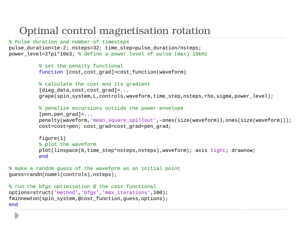
Optimal control magnetisation rotation % Pulse duration and number of timesteps
pulse_duration=1e-2; nsteps=32; time_step=pulse_duration/nsteps;
power_level=2*pi*10e3; % define a power level of pulse (max) 10kHz
% set the penalty functional
function [cost,cost_grad]=cost_function(waveform)
% calculate the cost and its gradient
[diag_data,cost,cost_grad]=...
grape(spin_system,L,controls,waveform,time_step,nsteps,rho,sigma,power_level);
% penalize excursions outside the power envelope
[pen,pen_grad]=...
penalty(waveform,'mean_square_spillout',-ones(size(waveform)),ones(size(waveform)));
cost=cost+pen; cost_grad=cost_grad+pen_grad;
figure(1)
% plot the waveform
plot(linspace(0,time_step*nsteps,nsteps),waveform); axis tight; drawnow;
end
% make a random guess of the waveform as an initial point
guess=randn(numel(controls),nsteps);
% run the bfgs optimisation @ the cost functional
options=struct('method','bfgs','max_iterations',100);
fminnewton(spin_system,@cost_function,guess,options);
end<br>
pulse_duration=1e-2; nsteps=32; time_step=pulse_duration/nsteps;
power_level=2*pi*10e3; % define a power level of pulse (max) 10kHz
% set the penalty functional
function [cost,cost_grad]=cost_function(waveform)
% calculate the cost and its gradient
[diag_data,cost,cost_grad]=...
grape(spin_system,L,controls,waveform,time_step,nsteps,rho,sigma,power_level);
% penalize excursions outside the power envelope
[pen,pen_grad]=...
penalty(waveform,'mean_square_spillout',-ones(size(waveform)),ones(size(waveform)));
cost=cost+pen; cost_grad=cost_grad+pen_grad;
figure(1)
% plot the waveform
plot(linspace(0,time_step*nsteps,nsteps),waveform); axis tight; drawnow;
end
% make a random guess of the waveform as an initial point
guess=randn(numel(controls),nsteps);
% run the bfgs optimisation @ the cost functional
options=struct('method','bfgs','max_iterations',100);
fminnewton(spin_system,@cost_function,guess,options);
end<br>
13
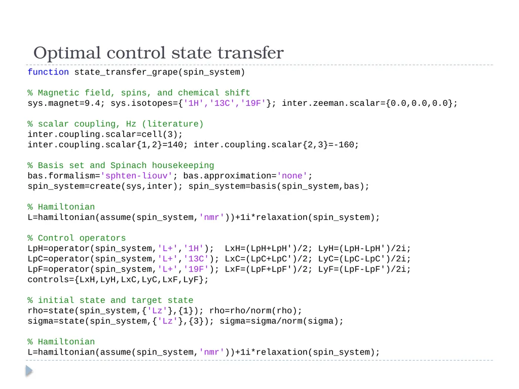
Optimal control state transfer function state_transfer_grape(spin_system)
% Magnetic field, spins, and chemical shift
sys.magnet=9.4; sys.isotopes={'1H','13C','19F'}; inter.zeeman.scalar={0.0,0.0,0.0};
% scalar coupling, Hz (literature)
inter.coupling.scalar=cell(3);
inter.coupling.scalar{1,2}=140; inter.coupling.scalar{2,3}=-160;
% Basis set and Spinach housekeeping
bas.formalism='sphten-liouv'; bas.approximation='none';
spin_system=create(sys,inter); spin_system=basis(spin_system,bas);
% Hamiltonian
L=hamiltonian(assume(spin_system,'nmr'))+1i*relaxation(spin_system);
% Control operators
LpH=operator(spin_system,'L+','1H'); LxH=(LpH+LpH')/2; LyH=(LpH-LpH')/2i;
LpC=operator(spin_system,'L+','13C'); LxC=(LpC+LpC')/2; LyC=(LpC-LpC')/2i;
LpF=operator(spin_system,'L+','19F'); LxF=(LpF+LpF')/2; LyF=(LpF-LpF')/2i;
controls={LxH,LyH,LxC,LyC,LxF,LyF};
% initial state and target state
rho=state(spin_system,{'Lz'},{1}); rho=rho/norm(rho);
sigma=state(spin_system,{'Lz'},{3}); sigma=sigma/norm(sigma);
% Hamiltonian
L=hamiltonian(assume(spin_system,'nmr'))+1i*relaxation(spin_system);<br>
% Magnetic field, spins, and chemical shift
sys.magnet=9.4; sys.isotopes={'1H','13C','19F'}; inter.zeeman.scalar={0.0,0.0,0.0};
% scalar coupling, Hz (literature)
inter.coupling.scalar=cell(3);
inter.coupling.scalar{1,2}=140; inter.coupling.scalar{2,3}=-160;
% Basis set and Spinach housekeeping
bas.formalism='sphten-liouv'; bas.approximation='none';
spin_system=create(sys,inter); spin_system=basis(spin_system,bas);
% Hamiltonian
L=hamiltonian(assume(spin_system,'nmr'))+1i*relaxation(spin_system);
% Control operators
LpH=operator(spin_system,'L+','1H'); LxH=(LpH+LpH')/2; LyH=(LpH-LpH')/2i;
LpC=operator(spin_system,'L+','13C'); LxC=(LpC+LpC')/2; LyC=(LpC-LpC')/2i;
LpF=operator(spin_system,'L+','19F'); LxF=(LpF+LpF')/2; LyF=(LpF-LpF')/2i;
controls={LxH,LyH,LxC,LyC,LxF,LyF};
% initial state and target state
rho=state(spin_system,{'Lz'},{1}); rho=rho/norm(rho);
sigma=state(spin_system,{'Lz'},{3}); sigma=sigma/norm(sigma);
% Hamiltonian
L=hamiltonian(assume(spin_system,'nmr'))+1i*relaxation(spin_system);<br>
14
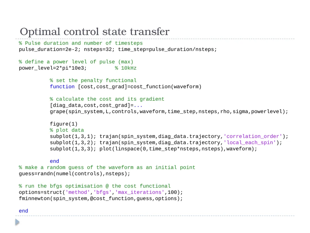
Optimal control state transfer % Pulse duration and number of timesteps
pulse_duration=2e-2; nsteps=32; time_step=pulse_duration/nsteps;
% define a power level of pulse (max)
power_level=2*pi*10e3; % 10kHz
% set the penalty functional
function [cost,cost_grad]=cost_function(waveform)
% calculate the cost and its gradient
[diag_data,cost,cost_grad]=...
grape(spin_system,L,controls,waveform,time_step,nsteps,rho,sigma,powerlevel);
figure(1)
% plot data
subplot(1,3,1); trajan(spin_system,diag_data.trajectory,'correlation_order');
subplot(1,3,2); trajan(spin_system,diag_data.trajectory,'local_each_spin');
subplot(1,3,3); plot(linspace(0,time_step*nsteps,nsteps),waveform);
end
% make a random guess of the waveform as an initial point
guess=randn(numel(controls),nsteps);
% run the bfgs optimisation @ the cost functional
options=struct('method','bfgs','max_iterations',100);
fminnewton(spin_system,@cost_function,guess,options);
end<br>
pulse_duration=2e-2; nsteps=32; time_step=pulse_duration/nsteps;
% define a power level of pulse (max)
power_level=2*pi*10e3; % 10kHz
% set the penalty functional
function [cost,cost_grad]=cost_function(waveform)
% calculate the cost and its gradient
[diag_data,cost,cost_grad]=...
grape(spin_system,L,controls,waveform,time_step,nsteps,rho,sigma,powerlevel);
figure(1)
% plot data
subplot(1,3,1); trajan(spin_system,diag_data.trajectory,'correlation_order');
subplot(1,3,2); trajan(spin_system,diag_data.trajectory,'local_each_spin');
subplot(1,3,3); plot(linspace(0,time_step*nsteps,nsteps),waveform);
end
% make a random guess of the waveform as an initial point
guess=randn(numel(controls),nsteps);
% run the bfgs optimisation @ the cost functional
options=struct('method','bfgs','max_iterations',100);
fminnewton(spin_system,@cost_function,guess,options);
end<br>
15
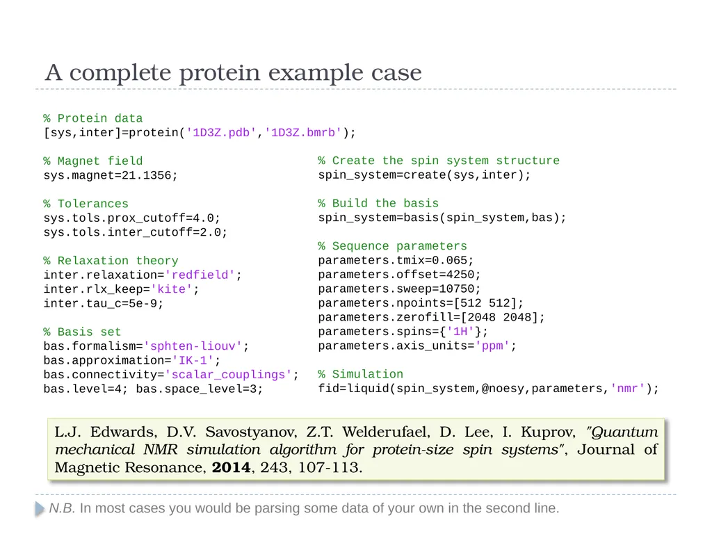
A complete protein example case N.B. In most cases you would be parsing some data of your own in the second line. % Protein data
[sys,inter]=protein('1D3Z.pdb','1D3Z.bmrb');
% Magnet field
sys.magnet=21.1356;
% Tolerances
sys.tols.prox_cutoff=4.0;
sys.tols.inter_cutoff=2.0;
% Relaxation theory
inter.relaxation='redfield';
inter.rlx_keep='kite';
inter.tau_c=5e-9;
% Basis set
bas.formalism='sphten-liouv';
bas.approximation='IK-1';
bas.connectivity='scalar_couplings';
bas.level=4; bas.space_level=3; L.J. Edwards, D.V. Savostyanov, Z.T. Welderufael, D. Lee, I. Kuprov, "Quantum mechanical NMR simulation algorithm for protein-size spin systems", Journal of Magnetic Resonance, 2014, 243, 107-113. % Create the spin system structure
spin_system=create(sys,inter);
% Build the basis
spin_system=basis(spin_system,bas);
% Sequence parameters
parameters.tmix=0.065;
parameters.offset=4250;
parameters.sweep=10750;
parameters.npoints=[512 512];
parameters.zerofill=[2048 2048];
parameters.spins={'1H'};
parameters.axis_units='ppm';
% Simulation
fid=liquid(spin_system,@noesy,parameters,'nmr');<br>
[sys,inter]=protein('1D3Z.pdb','1D3Z.bmrb');
% Magnet field
sys.magnet=21.1356;
% Tolerances
sys.tols.prox_cutoff=4.0;
sys.tols.inter_cutoff=2.0;
% Relaxation theory
inter.relaxation='redfield';
inter.rlx_keep='kite';
inter.tau_c=5e-9;
% Basis set
bas.formalism='sphten-liouv';
bas.approximation='IK-1';
bas.connectivity='scalar_couplings';
bas.level=4; bas.space_level=3; L.J. Edwards, D.V. Savostyanov, Z.T. Welderufael, D. Lee, I. Kuprov, "Quantum mechanical NMR simulation algorithm for protein-size spin systems", Journal of Magnetic Resonance, 2014, 243, 107-113. % Create the spin system structure
spin_system=create(sys,inter);
% Build the basis
spin_system=basis(spin_system,bas);
% Sequence parameters
parameters.tmix=0.065;
parameters.offset=4250;
parameters.sweep=10750;
parameters.npoints=[512 512];
parameters.zerofill=[2048 2048];
parameters.spins={'1H'};
parameters.axis_units='ppm';
% Simulation
fid=liquid(spin_system,@noesy,parameters,'nmr');<br>
16
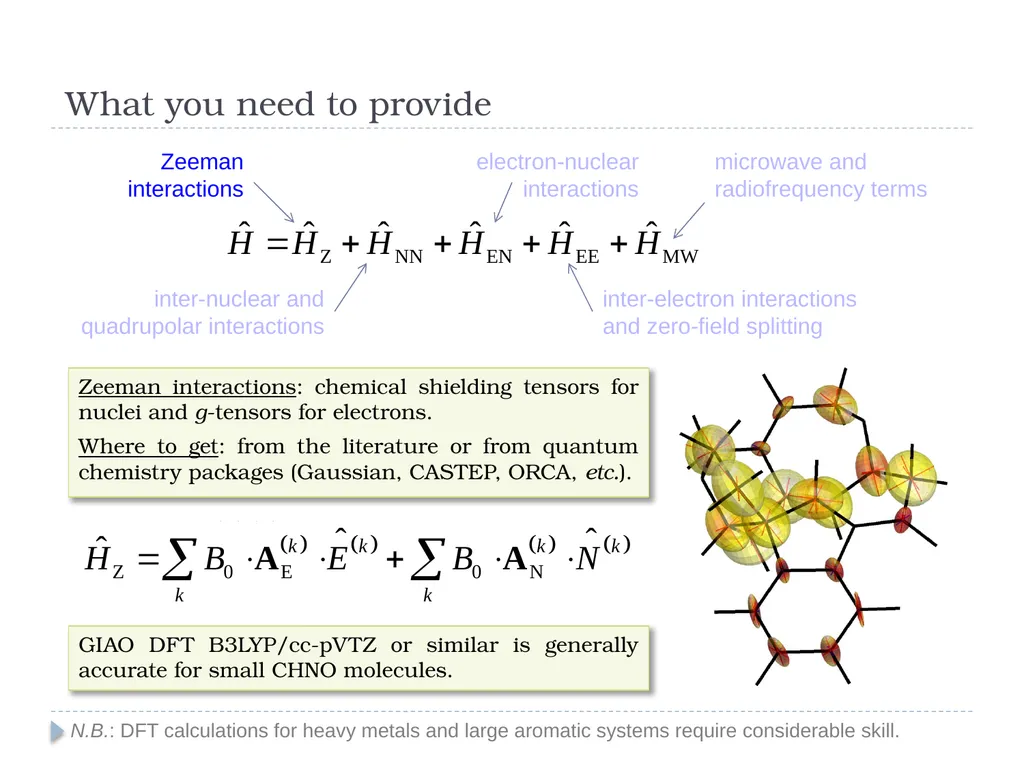
What you need to provide N.B.: DFT calculations for heavy metals and large aromatic systems require considerable skill. Zeeman interactions inter-nuclear and quadrupolar interactions electron-nuclear
interactions inter-electron interactions
and zero-field splitting microwave and radiofrequency terms Zeeman interactions: chemical shielding tensors for nuclei and g-tensors for electrons.
Where to get: from the literature or from quantum chemistry packages (Gaussian, CASTEP, ORCA, etc.). GIAO DFT B3LYP/cc-pVTZ or similar is generally accurate for small CHNO molecules.<br>
Where to get: from the literature or from quantum chemistry packages (Gaussian, CASTEP, ORCA, etc.). GIAO DFT B3LYP/cc-pVTZ or similar is generally accurate for small CHNO molecules.<br>
17
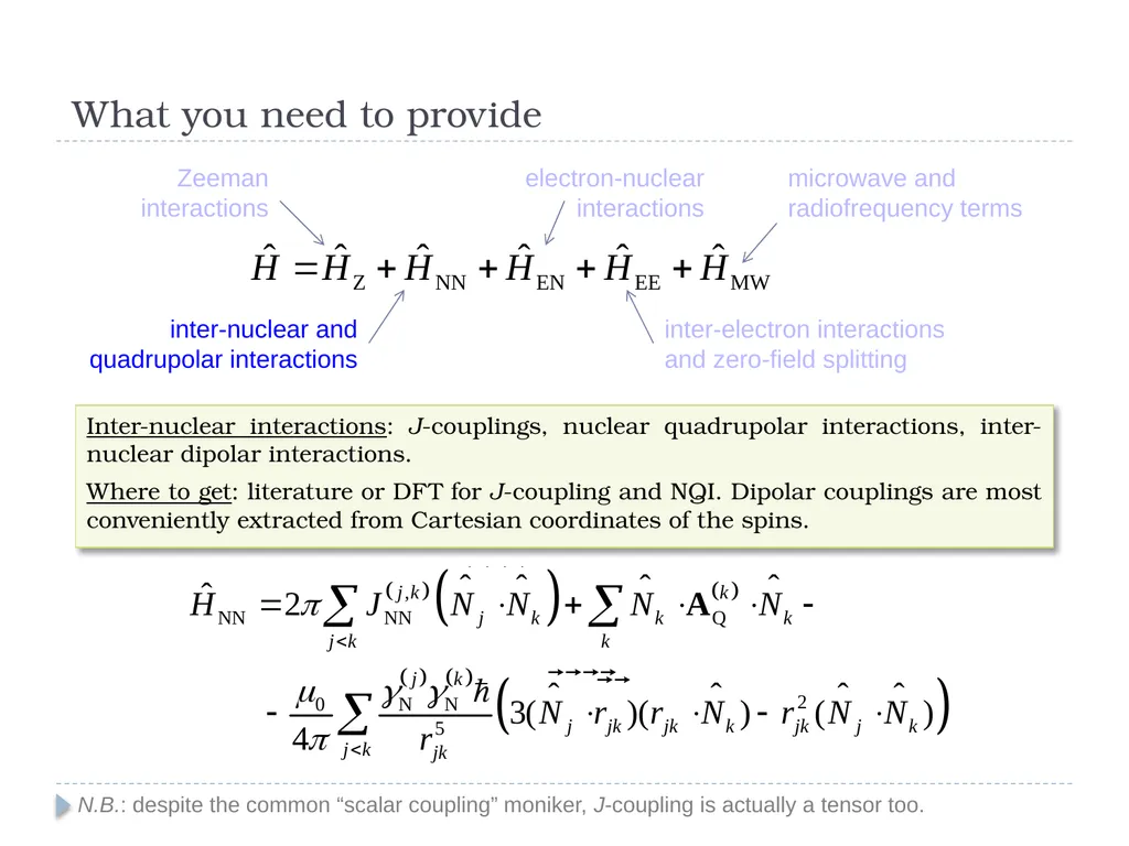
What you need to provide N.B.: despite the common “scalar coupling” moniker, J-coupling is actually a tensor too. Zeeman interactions inter-nuclear and quadrupolar interactions electron-nuclear
interactions inter-electron interactions
and zero-field splitting microwave and radiofrequency terms Inter-nuclear interactions: J-couplings, nuclear quadrupolar interactions, inter-nuclear dipolar interactions.
Where to get: literature or DFT for J-coupling and NQI. Dipolar couplings are most conveniently extracted from Cartesian coordinates of the spins.<br>
Where to get: literature or DFT for J-coupling and NQI. Dipolar couplings are most conveniently extracted from Cartesian coordinates of the spins.<br>
18
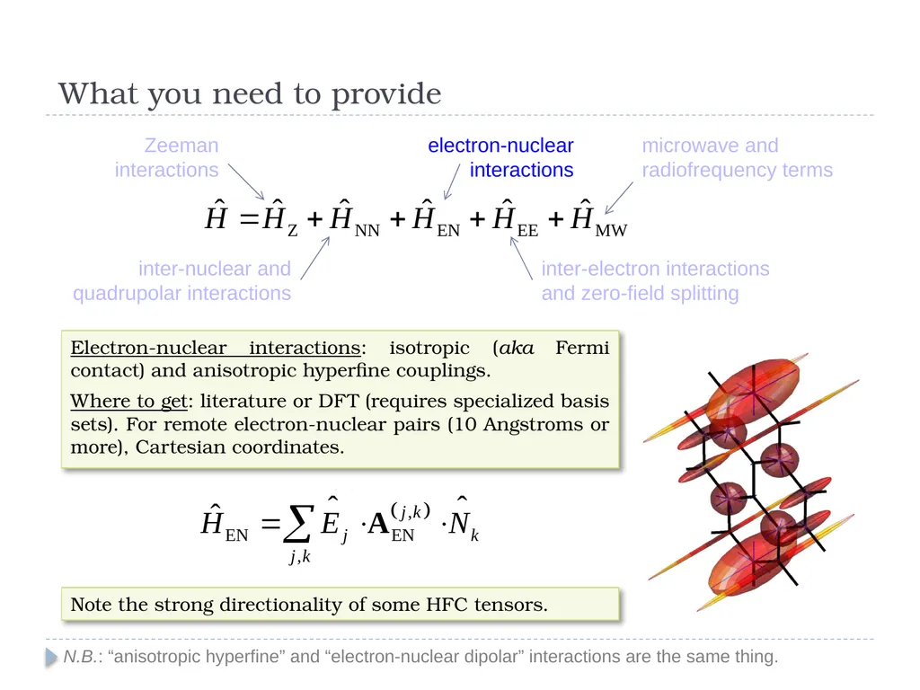
What you need to provide N.B.: “anisotropic hyperfine” and “electron-nuclear dipolar” interactions are the same thing. Zeeman interactions inter-nuclear and quadrupolar interactions electron-nuclear
interactions inter-electron interactions
and zero-field splitting microwave and radiofrequency terms Electron-nuclear interactions: isotropic (aka Fermi contact) and anisotropic hyperfine couplings.
Where to get: literature or DFT (requires specialized basis sets). For remote electron-nuclear pairs (10 Angstroms or more), Cartesian coordinates. Note the strong directionality of some HFC tensors.<br>
Where to get: literature or DFT (requires specialized basis sets). For remote electron-nuclear pairs (10 Angstroms or more), Cartesian coordinates. Note the strong directionality of some HFC tensors.<br>
19
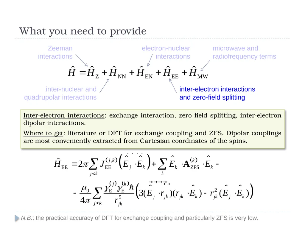
What you need to provide N.B.: the practical accuracy of DFT for exchange coupling and particularly ZFS is very low. Zeeman interactions inter-nuclear and quadrupolar interactions electron-nuclear
interactions inter-electron interactions
and zero-field splitting microwave and radiofrequency terms Inter-electron interactions: exchange interaction, zero field splitting, inter-electron dipolar interactions.
Where to get: literature or DFT for exchange coupling and ZFS. Dipolar couplings are most conveniently extracted from Cartesian coordinates of the spins.<br>
Where to get: literature or DFT for exchange coupling and ZFS. Dipolar couplings are most conveniently extracted from Cartesian coordinates of the spins.<br>
20
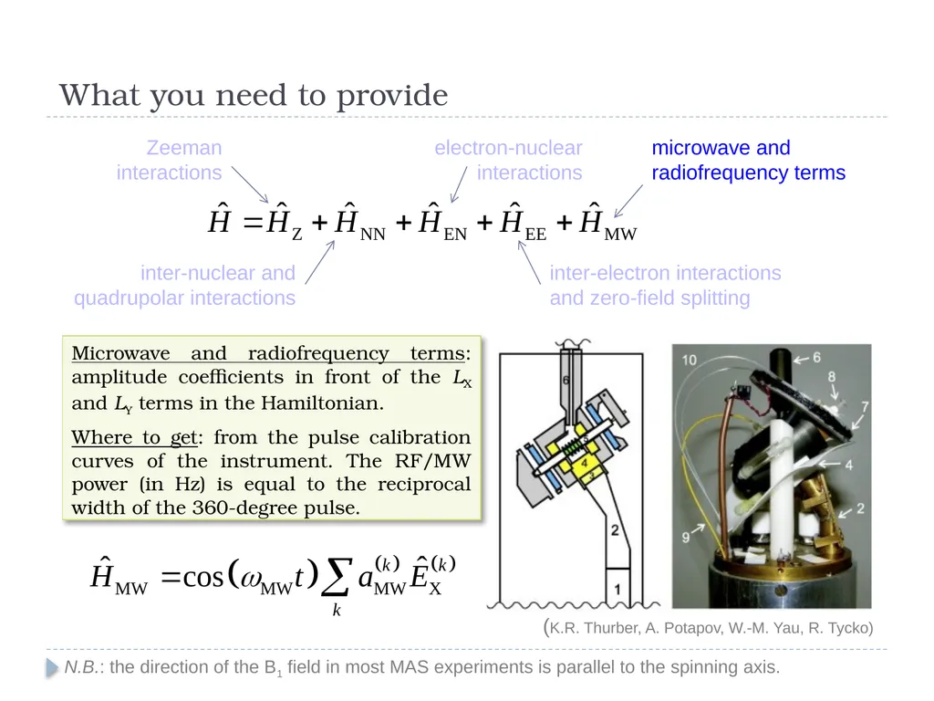
What you need to provide N.B.: the direction of the B1 field in most MAS experiments is parallel to the spinning axis. Zeeman interactions inter-nuclear and quadrupolar interactions electron-nuclear
interactions inter-electron interactions
and zero-field splitting microwave and radiofrequency terms Microwave and radiofrequency terms: amplitude coefficients in front of the LX and LY terms in the Hamiltonian.
Where to get: from the pulse calibration curves of the instrument. The RF/MW power (in Hz) is equal to the reciprocal width of the 360-degree pulse. (K.R. Thurber, A. Potapov, W.-M. Yau, R. Tycko)<br>
Where to get: from the pulse calibration curves of the instrument. The RF/MW power (in Hz) is equal to the reciprocal width of the 360-degree pulse. (K.R. Thurber, A. Potapov, W.-M. Yau, R. Tycko)<br>