
UNIT IV Decision Making by: Dr. Pravin Kumar




Description: UNIT IV Decision Making by: Dr. Pravin Kumar Agrawal Assistant Professor CSJMU Decision-Making Decision-making is needed whenever an individual or an organization (private or public) is faced with a situation of selecting an optimal (or
Related Topics
Download Presentation
"UNIT IV Decision Making by: Dr. Pravin Kumar" is the property of its rightful owner. Permission is granted to download and print the materials on this website for personal, non-commercial use only, and to display it on your personal computer provided you do not modify the materials and that you retain all copyright notices contained in the materials. By downloading content from our website, you accept the terms of this agreement.
Presentation Transcript
slide1. UNIT IV Decision Making
by:
Dr. Pravin Kumar Agrawal
Assistant Professor
CSJMU<br>
slide2. Decision-Making Decision-making is needed whenever an individual or an organization (private or public) is faced with a situation of selecting an optimal (or best in view of certain objectives) course of action from among several available alternatives.
For example, an individual may have to decide whether to build a house or to purchase a flat or live in a rented accommodation; whether to join a service or to start own business; which company's car should be purchased, etc. Similarly, a business firm may have to decide the type of technique to be used in production, what is the most appropriate method of advertising its product, etc.
The decision analysis provides certain criteria for the selection of a course of action such that the objective of the decision-maker is satisfied. The course of action selected on the basis of such criteria is termed as the optimal course of action.<br>
slide3. Decision Alternatives Every decision-maker is faced with a set of several alternative courses of action A1, A2, ...... Am and he has to select one of them in view of the objectives to be fulfilled.<br>
slide4. States of Nature These are the future conditions that are not under the control of decision – maker.
A state of nature can be the state of economy (e.g. inflation), a weather condition etc. The state of nature are usually not determined by the action of an individual or an organization, These are the results of an “act of GOD”<br>
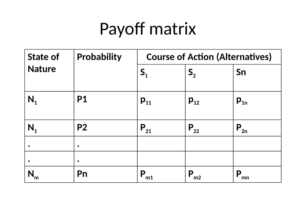
slide5. Payoff A numerical value (outcome) resulting from each possible combination of alternatives and state of nature is called pay The payoff values are always conditional values because of unknown states of nature.
Measured within a specified period (e.g. after one year). This period is called as the decision horizon.<br>
slide6. Payoff matrix<br>
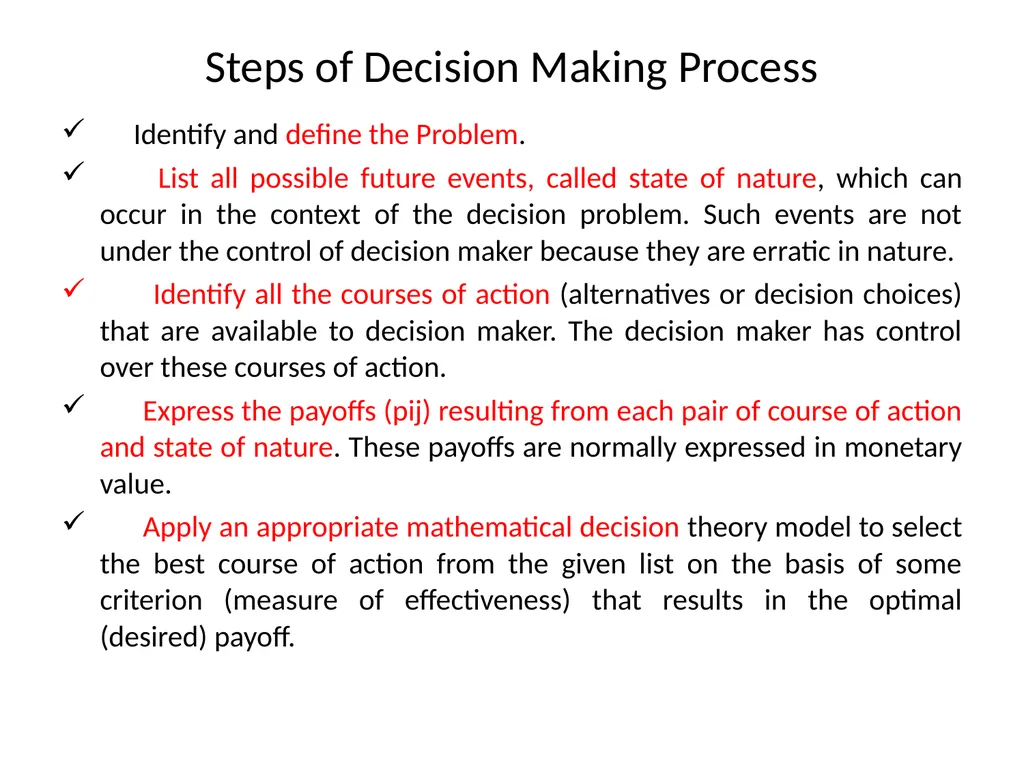
slide7. Steps of Decision Making Process Identify and define the Problem.
List all possible future events, called state of nature, which can occur in the context of the decision problem. Such events are not under the control of decision maker because they are erratic in nature.
Identify all the courses of action (alternatives or decision choices) that are available to decision maker. The decision maker has control over these courses of action.
Express the payoffs (pij) resulting from each pair of course of action and state of nature. These payoffs are normally expressed in monetary value.
Apply an appropriate mathematical decision theory model to select the best course of action from the given list on the basis of some criterion (measure of effectiveness) that results in the optimal (desired) payoff.<br>
slide8. Types of Decision Making Environments<br>
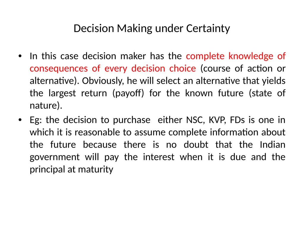
slide9. Decision Making under Certainty In this case decision maker has the complete knowledge of consequences of every decision choice (course of action or alternative). Obviously, he will select an alternative that yields the largest return (payoff) for the known future (state of nature).
Eg: the decision to purchase either NSC, KVP, FDs is one in which it is reasonable to assume complete information about the future because there is no doubt that the Indian government will pay the interest when it is due and the principal at maturity<br>
slide10. Decision Making under Risk In this case the decision maker has less than complete knowledge of the consequences of every decision choice (course of action). This is because it is not definitely known which outcome will occur. This means there is one state of nature (future) and for which he makes an assumption of the probability with which each state of nature will occur. Eg product demand high, low, medium.<br>
slide11. Decision Making under Uncertainty A decision problem, where a decision-maker is aware of various possible states of nature but has insufficient information to assign any probabilities of occurrence to them, is termed as decision-making under uncertainty.
A situation of uncertainty arises when there can be more than one possible consequences of selecting any course of action. In terms of the payoff matrix, if the decision-maker selects A1, his payoff can be X11, X12, X13, etc., depending upon which state of nature S1, S2, S3, etc., is going to occur.<br>
slide12. Most significant decisions made in today’s complex environment are formulated under a state of uncertainty. Conditions of uncertainty exist when the future environment is unpredictable. The decision-maker is not aware of all available alternatives, the risks associated with each, and the consequences of each alternative or their probabilities.
The manager does not possess complete information about the alternatives and whatever information is available, may not be completely reliable. In the face of such uncertainty, managers need to make certain assumptions about the situation in order to provide a reasonable framework for decision-making. They have to depend upon their judgment and experience for making decisions.<br>
slide13. Decision making under Uncertainty Optimism (Maximax or Minimin) criterion (2018-19)
Pessimism (Maximin or Minimax) criterion (2018-19)
Equal Probabilities (Laplace) criterion
Coefficeint of optimism (Hurwicz) criterion
Regret (Salvage) criterion<br>
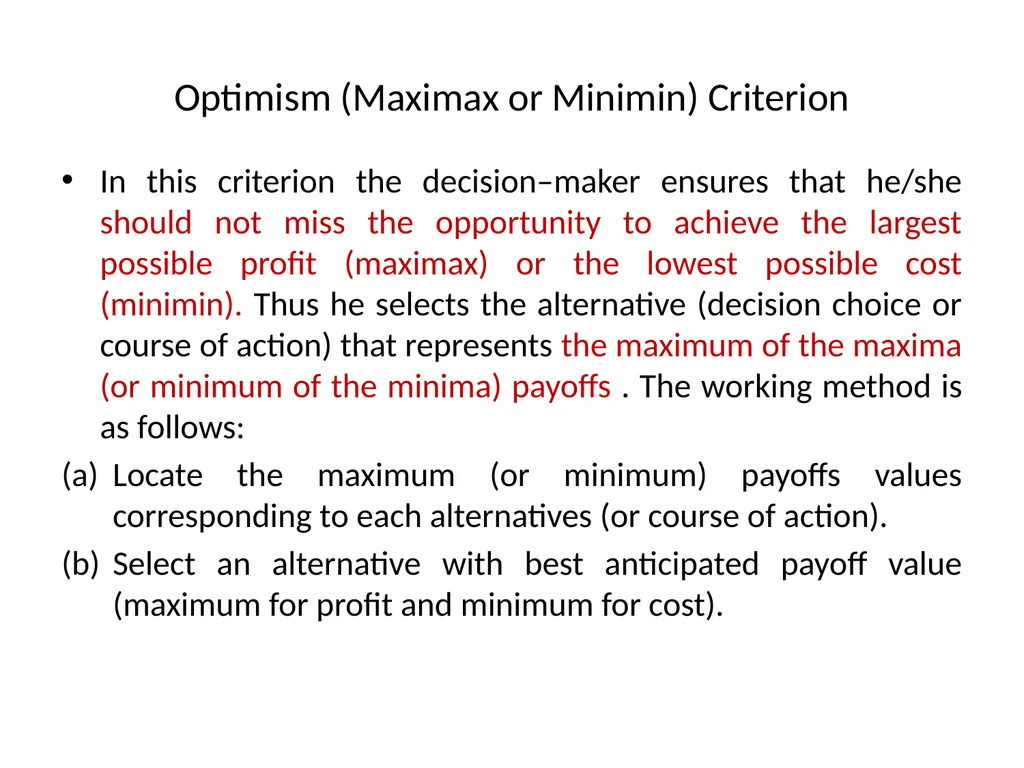
slide14. Optimism (Maximax or Minimin) Criterion In this criterion the decision–maker ensures that he/she should not miss the opportunity to achieve the largest possible profit (maximax) or the lowest possible cost (minimin). Thus he selects the alternative (decision choice or course of action) that represents the maximum of the maxima (or minimum of the minima) payoffs . The working method is as follows:
Locate the maximum (or minimum) payoffs values corresponding to each alternatives (or course of action).
Select an alternative with best anticipated payoff value (maximum for profit and minimum for cost).<br>
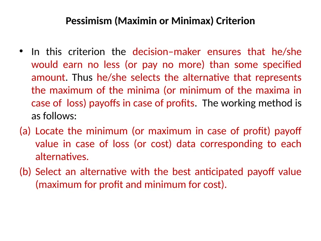
slide15. Pessimism (Maximin or Minimax) Criterion In this criterion the decision–maker ensures that he/she would earn no less (or pay no more) than some specified amount. Thus he/she selects the alternative that represents the maximum of the minima (or minimum of the maxima in case of loss) payoffs in case of profits. The working method is as follows:
Locate the minimum (or maximum in case of profit) payoff value in case of loss (or cost) data corresponding to each alternatives.
Select an alternative with the best anticipated payoff value (maximum for profit and minimum for cost).<br>
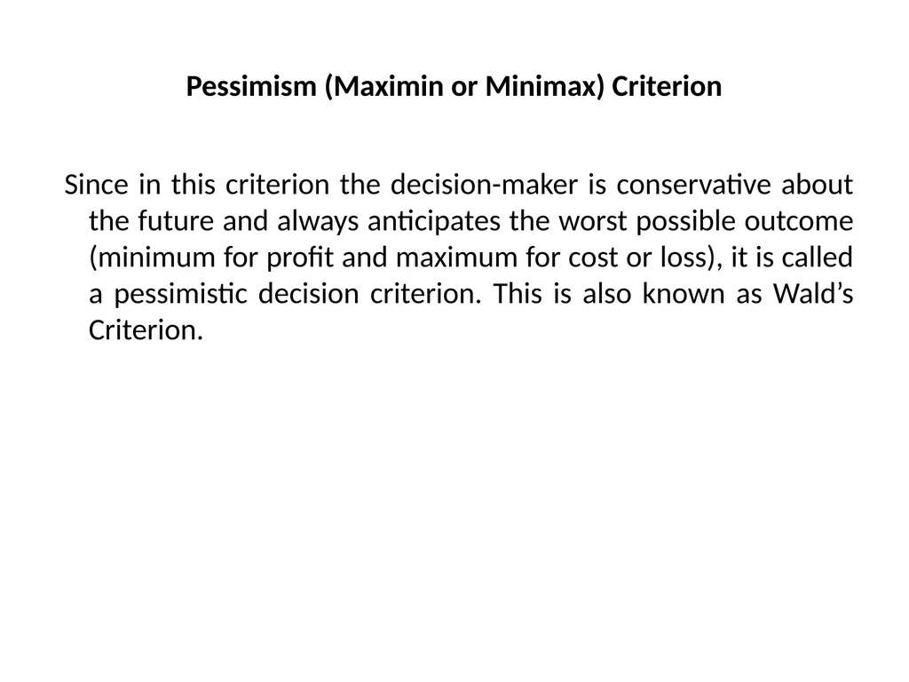
slide16. Pessimism (Maximin or Minimax) Criterion Since in this criterion the decision-maker is conservative about the future and always anticipates the worst possible outcome (minimum for profit and maximum for cost or loss), it is called a pessimistic decision criterion. This is also known as Wald’s Criterion.<br>
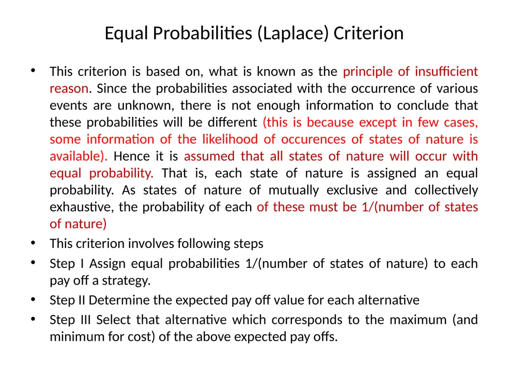
slide17. Equal Probabilities (Laplace) Criterion This criterion is based on, what is known as the principle of insufficient reason. Since the probabilities associated with the occurrence of various events are unknown, there is not enough information to conclude that these probabilities will be different (this is because except in few cases, some information of the likelihood of occurences of states of nature is available). Hence it is assumed that all states of nature will occur with equal probability. That is, each state of nature is assigned an equal probability. As states of nature of mutually exclusive and collectively exhaustive, the probability of each of these must be 1/(number of states of nature)
This criterion involves following steps
Step I Assign equal probabilities 1/(number of states of nature) to each pay off a strategy.
Step II Determine the expected pay off value for each alternative
Step III Select that alternative which corresponds to the maximum (and minimum for cost) of the above expected pay offs.<br>
slide18. Coefficient of Optimism (Hurwicz) Criterion This criterion suggests that a rational decision maker should neither be completely optimistic nor be pessimistic and therefore, must display a mixture of both. Hurwicz, who suggests this criterion, introduced the idea of a coefficient of optimism (denoted by α) to measure the decision maker’s degree of optimism. This coefficient lies between 0 and 1, where 0 represents a completely pessimistic attitude about the future and 1, completely optimistic attitude about the future. Thus, if it is the coefficient of optimism, then (1- α ) will represent the coefficient of pessimism. The working procedure is –<br>
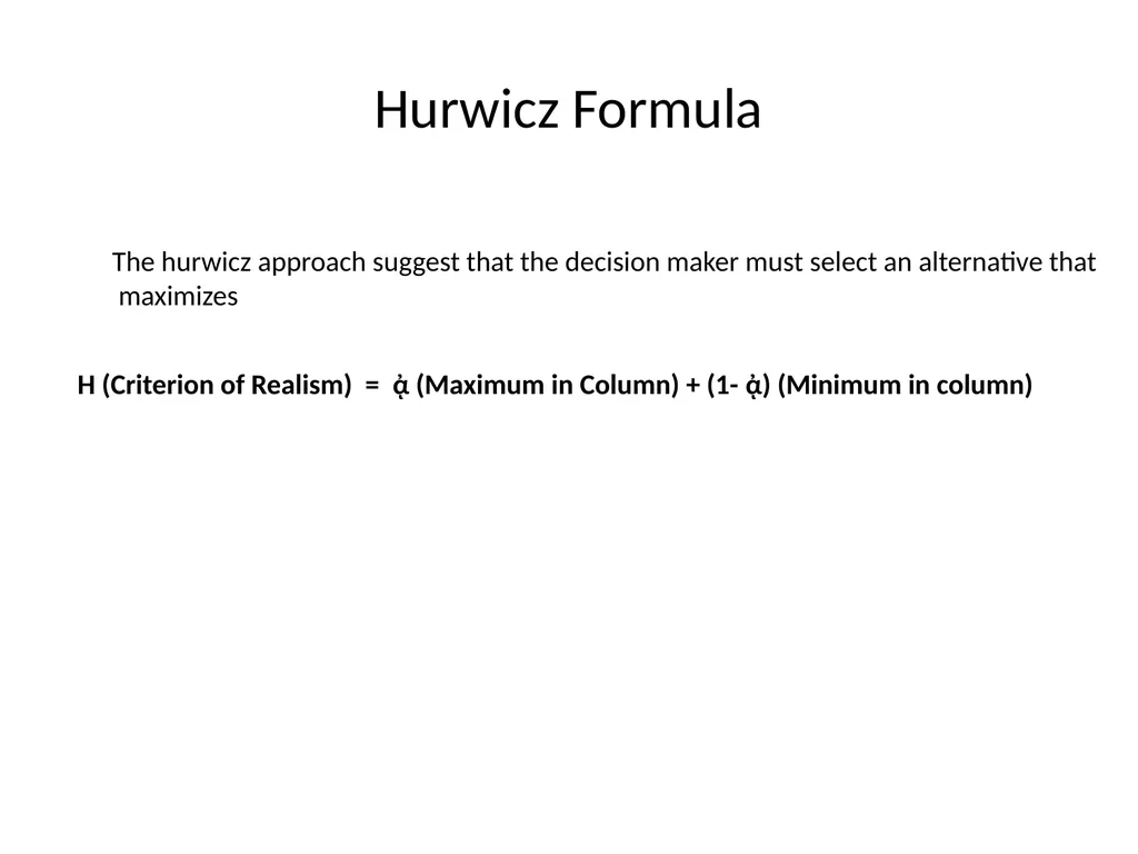
slide19. Hurwicz Formula H (Criterion of Realism) = ᾀ (Maximum in Column) + (1- ᾀ) (Minimum in column) The hurwicz approach suggest that the decision maker must select an alternative that
maximizes<br>
slide20. Coefficient of Optimism (Hurwicz) Criterion Select an alternative with value of H as maximum.
For α=1, the Hurwitz criteria is equal to the maximin or minimax criteria.
For α = 0, it is equal to maximax or minimin criteria.
A difficulty with this criteria is the appropriate selection of α between 0 and 1<br>
slide21. Regret (Salvage) Criterion While the above criterions do not take into account the cost of opportunity loses by making the wrong decision, the Savage criterion does so. The savage criterion is based on the concept of regret (or opportunity loss) and calls for selecting the course of action that minimizes the maximum regret. This criterion is assume that decision maker feels regret after adopting a wrong course of action (alternative) resulting in an opportunity loss of pay off. The working method is as follows:<br>
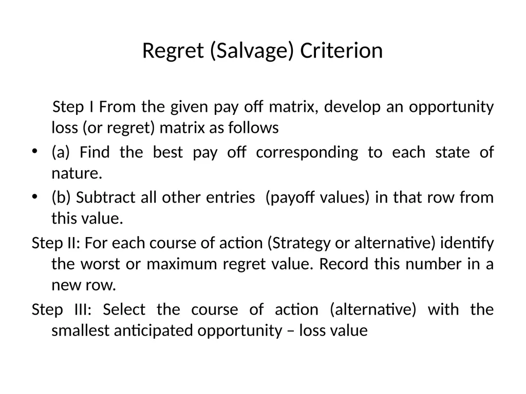
slide22. Regret (Salvage) Criterion Step I From the given pay off matrix, develop an opportunity loss (or regret) matrix as follows
(a) Find the best pay off corresponding to each state of nature.
(b) Subtract all other entries (payoff values) in that row from this value.
Step II: For each course of action (Strategy or alternative) identify the worst or maximum regret value. Record this number in a new row.
Step III: Select the course of action (alternative) with the smallest anticipated opportunity – loss value<br>
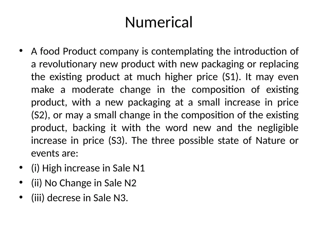
slide23. Numerical A food Product company is contemplating the introduction of a revolutionary new product with new packaging or replacing the existing product at much higher price (S1). It may even make a moderate change in the composition of existing product, with a new packaging at a small increase in price (S2), or may a small change in the composition of the existing product, backing it with the word new and the negligible increase in price (S3). The three possible state of Nature or events are:
(i) High increase in Sale N1
(ii) No Change in Sale N2
(iii) decrese in Sale N3.<br>
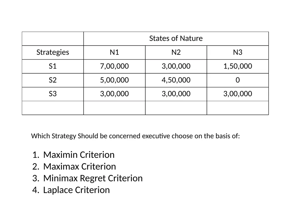
slide24. The marketing department of the company worked out the payoffs in terms of yearly net profits for each of the strategies of three events (expected sales). This is represented in the following table:<br>
slide25. Which Strategy Should be concerned executive choose on the basis of: Maximin Criterion
Maximax Criterion
Minimax Regret Criterion
Laplace Criterion<br>
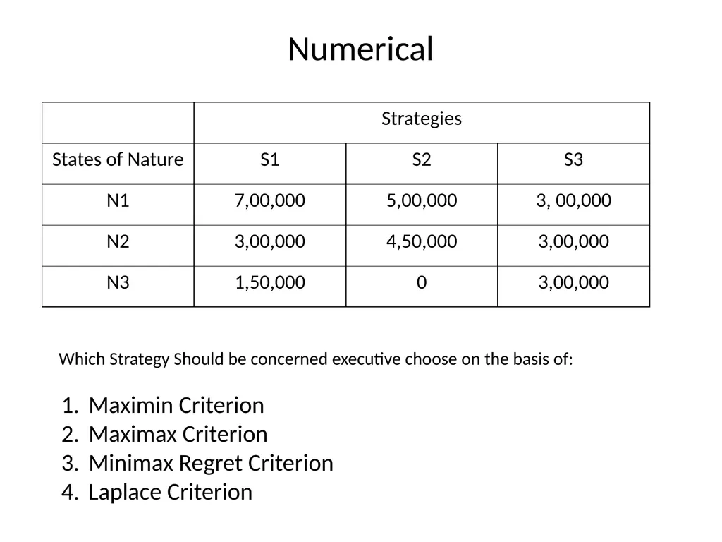
slide26. Numerical Which Strategy Should be concerned executive choose on the basis of: Maximin Criterion
Maximax Criterion
Minimax Regret Criterion
Laplace Criterion<br>
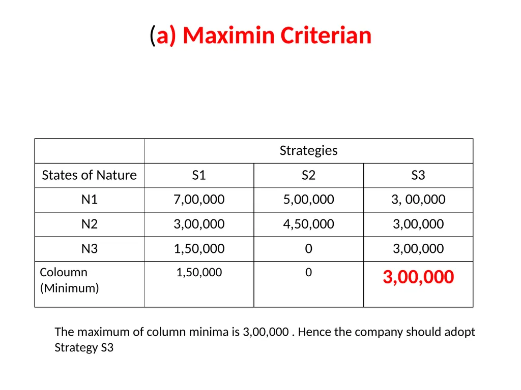
slide27. (a) Maximin Criterian The maximum of column minima is 3,00,000 . Hence the company should adopt
Strategy S3<br>
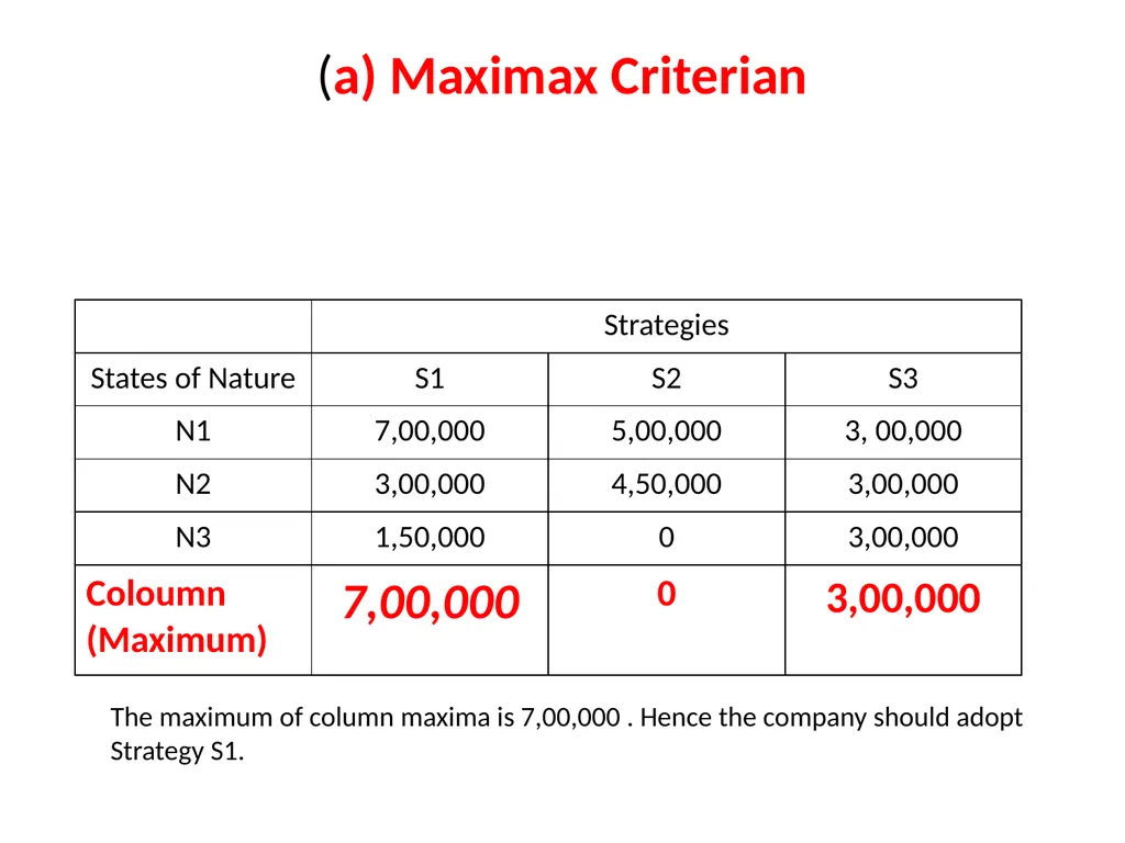
slide28. (a) Maximax Criterian The maximum of column maxima is 7,00,000 . Hence the company should adopt
Strategy S1.<br>
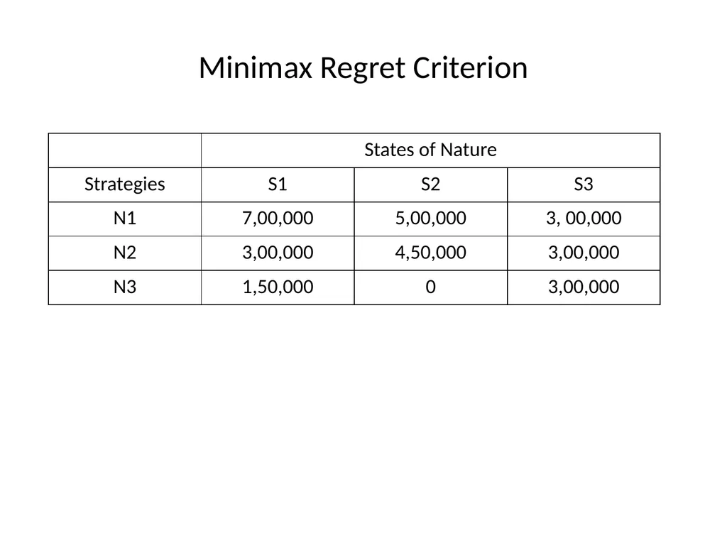
slide29. Minimax Regret Criterion<br>
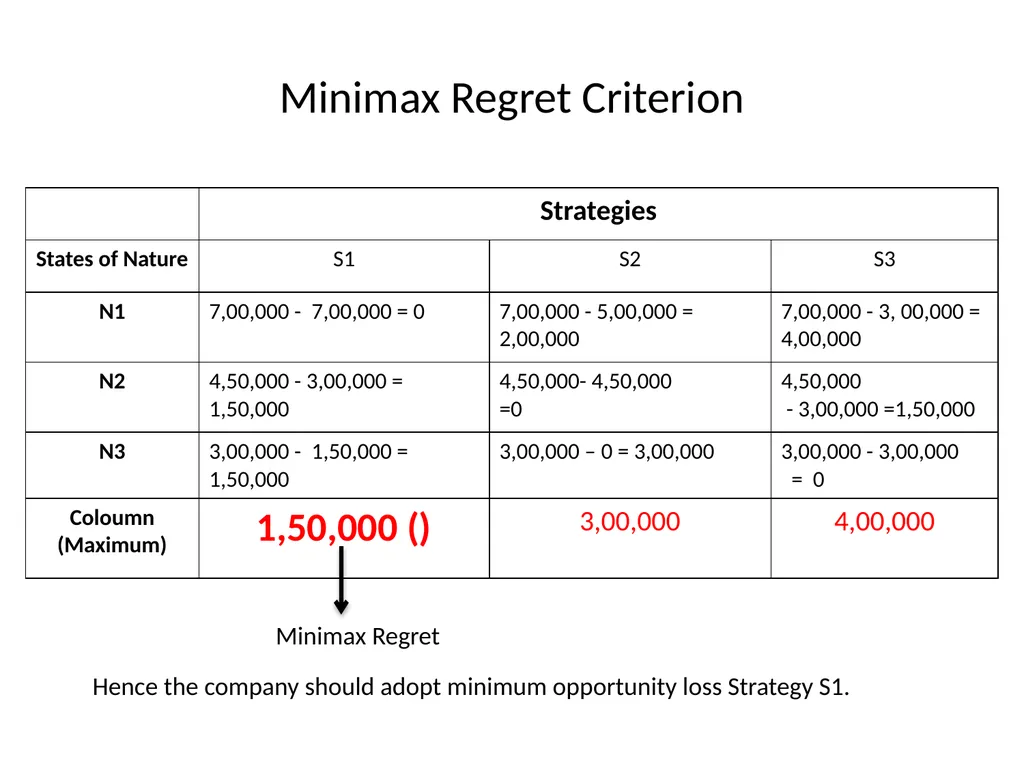
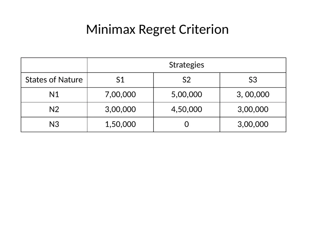
slide30. Minimax Regret Criterion Hence the company should adopt minimum opportunity loss Strategy S1. Minimax Regret<br>
slide31. Laplace Criterion Since we do not know the probabilities of State of nature, assume that they are equal. In this example we assume that each state of nature has a probability of 1/3 occurrence. Thus<br>
slide32. Minimax Regret Criterion<br>
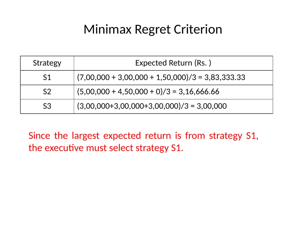
slide33. Minimax Regret Criterion Since the largest expected return is from strategy S1, the executive must select strategy S1.<br>
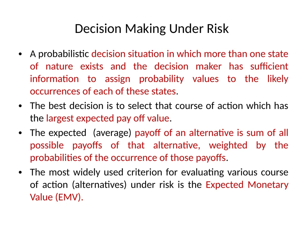
slide34. Decision Making Under Risk A probabilistic decision situation in which more than one state of nature exists and the decision maker has sufficient information to assign probability values to the likely occurrences of each of these states.
The best decision is to select that course of action which has the largest expected pay off value.
The expected (average) payoff of an alternative is sum of all possible payoffs of that alternative, weighted by the probabilities of the occurrence of those payoffs.
The most widely used criterion for evaluating various course of action (alternatives) under risk is the Expected Monetary Value (EMV).<br>
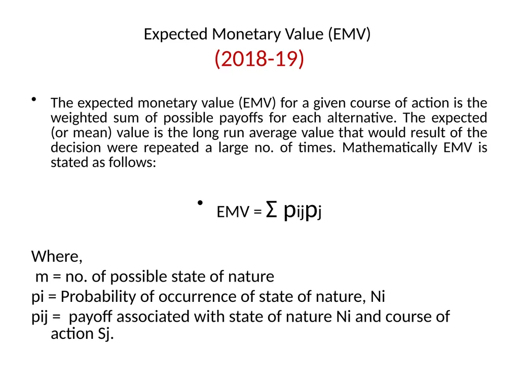
slide35. Expected Monetary Value (EMV) (2018-19) The expected monetary value (EMV) for a given course of action is the weighted sum of possible payoffs for each alternative. The expected (or mean) value is the long run average value that would result of the decision were repeated a large no. of times. Mathematically EMV is stated as follows:
EMV = Ʃ pijpj
Where,
m = no. of possible state of nature
pi = Probability of occurrence of state of nature, Ni
pij = payoff associated with state of nature Ni and course of action Sj.<br>
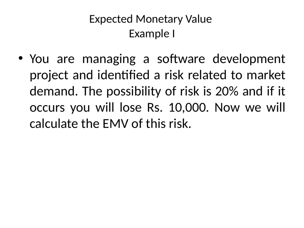
slide36. Expected Monetary Value Example I You are managing a software development project and identified a risk related to market demand. The possibility of risk is 20% and if it occurs you will lose Rs. 10,000. Now we will calculate the EMV of this risk.<br>
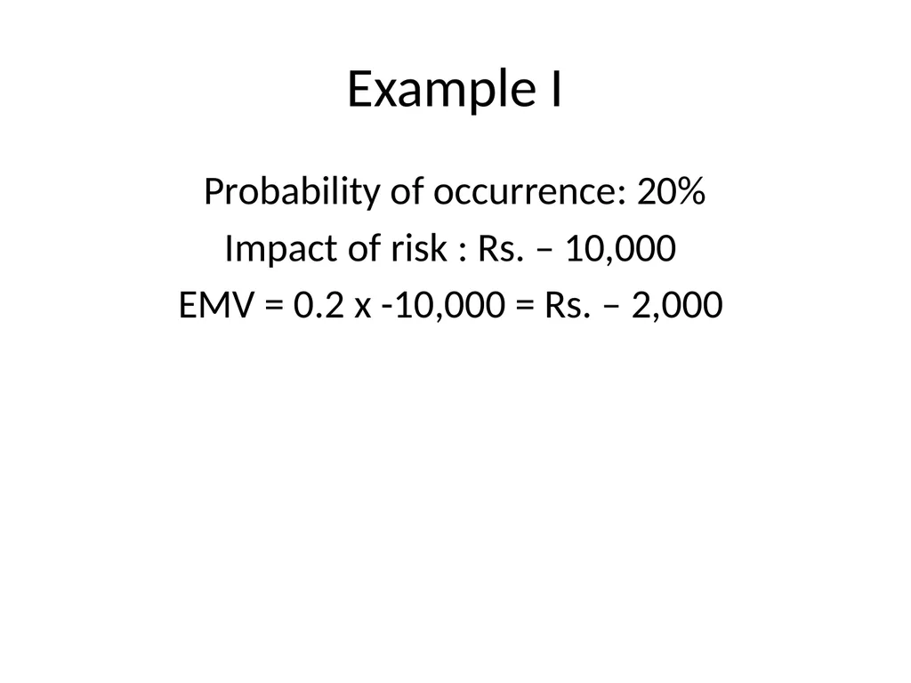
slide37. Example I Probability of occurrence: 20%
Impact of risk : Rs. – 10,000
EMV = 0.2 x -10,000 = Rs. – 2,000<br>
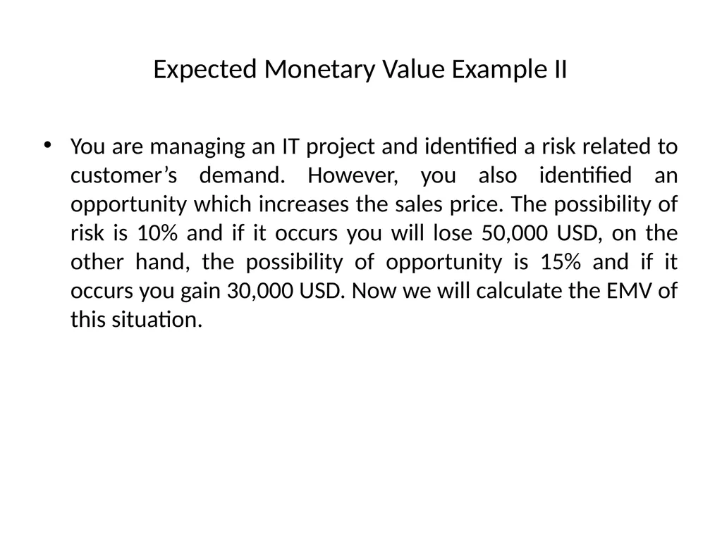
slide38. Expected Monetary Value Example II You are managing an IT project and identified a risk related to customer’s demand. However, you also identified an opportunity which increases the sales price. The possibility of risk is 10% and if it occurs you will lose 50,000 USD, on the other hand, the possibility of opportunity is 15% and if it occurs you gain 30,000 USD. Now we will calculate the EMV of this situation.<br>
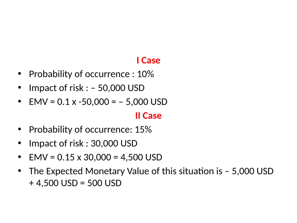
slide39. I Case
Probability of occurrence : 10%
Impact of risk : – 50,000 USD
EMV = 0.1 x -50,000 = – 5,000 USD
II Case
Probability of occurrence: 15%
Impact of risk : 30,000 USD
EMV = 0.15 x 30,000 = 4,500 USD
The Expected Monetary Value of this situation is – 5,000 USD + 4,500 USD = 500 USD<br>
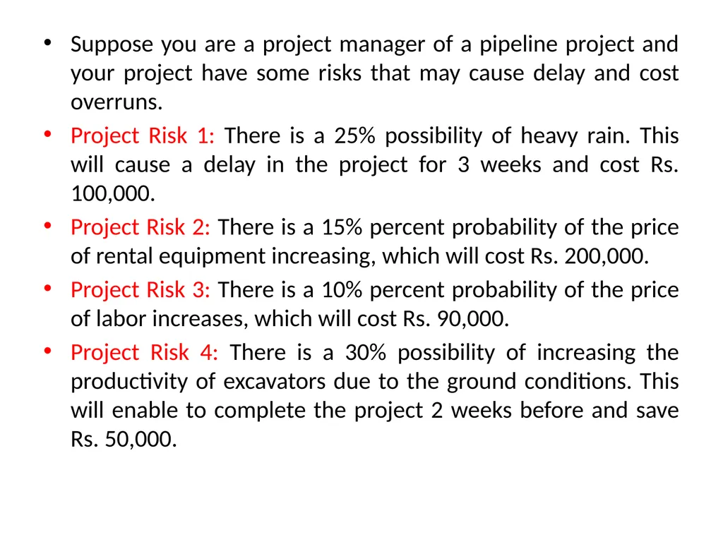
slide40. Suppose you are a project manager of a pipeline project and your project have some risks that may cause delay and cost overruns.
Project Risk 1: There is a 25% possibility of heavy rain. This will cause a delay in the project for 3 weeks and cost Rs. 100,000.
Project Risk 2: There is a 15% percent probability of the price of rental equipment increasing, which will cost Rs. 200,000.
Project Risk 3: There is a 10% percent probability of the price of labor increases, which will cost Rs. 90,000.
Project Risk 4: There is a 30% possibility of increasing the productivity of excavators due to the ground conditions. This will enable to complete the project 2 weeks before and save Rs. 50,000.<br>
slide41. Now Let’s calculate the EMV of the project In this scenario, the project manager should add Rs. 49,000 to the project budget to
manage those risks.<br>
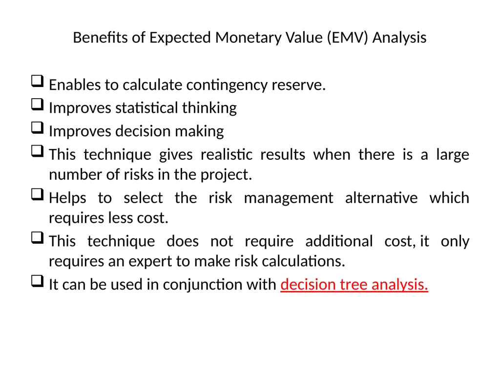
slide42. Benefits of Expected Monetary Value (EMV) Analysis Enables to calculate contingency reserve.
Improves statistical thinking
Improves decision making
This technique gives realistic results when there is a large number of risks in the project.
Helps to select the risk management alternative which requires less cost.
This technique does not require additional cost, it only requires an expert to make risk calculations.
It can be used in conjunction with decision tree analysis.<br>
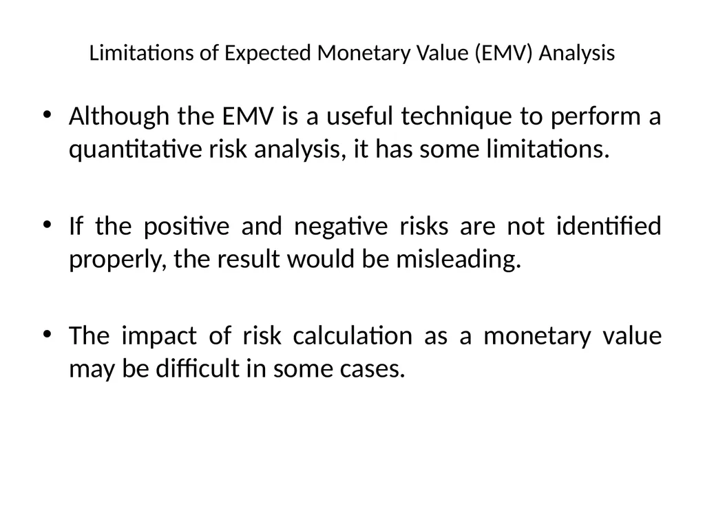
slide43. Limitations of Expected Monetary Value (EMV) Analysis Although the EMV is a useful technique to perform a quantitative risk analysis, it has some limitations.
If the positive and negative risks are not identified properly, the result would be misleading.
The impact of risk calculation as a monetary value may be difficult in some cases.<br>
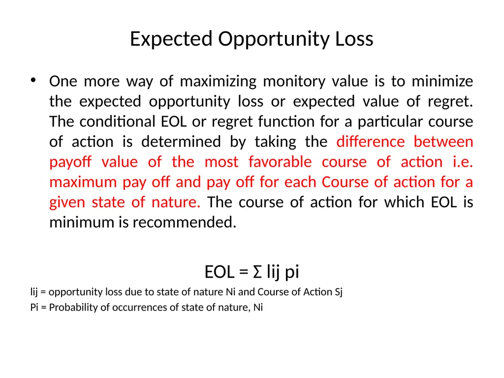
slide44. Expected Opportunity Loss One more way of maximizing monitory value is to minimize the expected opportunity loss or expected value of regret. The conditional EOL or regret function for a particular course of action is determined by taking the difference between payoff value of the most favorable course of action i.e. maximum pay off and pay off for each Course of action for a given state of nature. The course of action for which EOL is minimum is recommended.
EOL = Ʃ lij pi
lij = opportunity loss due to state of nature Ni and Course of Action Sj
Pi = Probability of occurrences of state of nature, Ni<br>
slide45. https://www.coursehero.com/file/p2losa4/Decision-Making-under-Risk-Expected-Opportunity-Loss-EOL-Another-useful-way-of/<br>
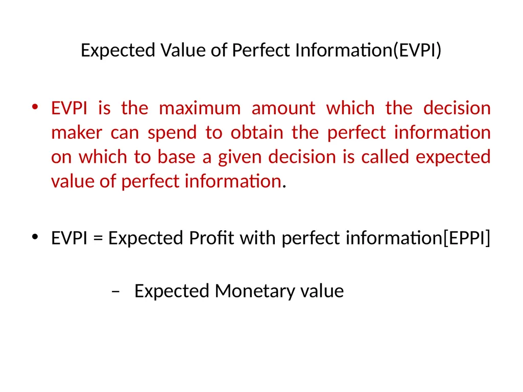
slide46. Expected Value of Perfect Information(EVPI) EVPI is the maximum amount which the decision maker can spend to obtain the perfect information on which to base a given decision is called expected value of perfect information.
EVPI = Expected Profit with perfect information[EPPI]
– Expected Monetary value<br>
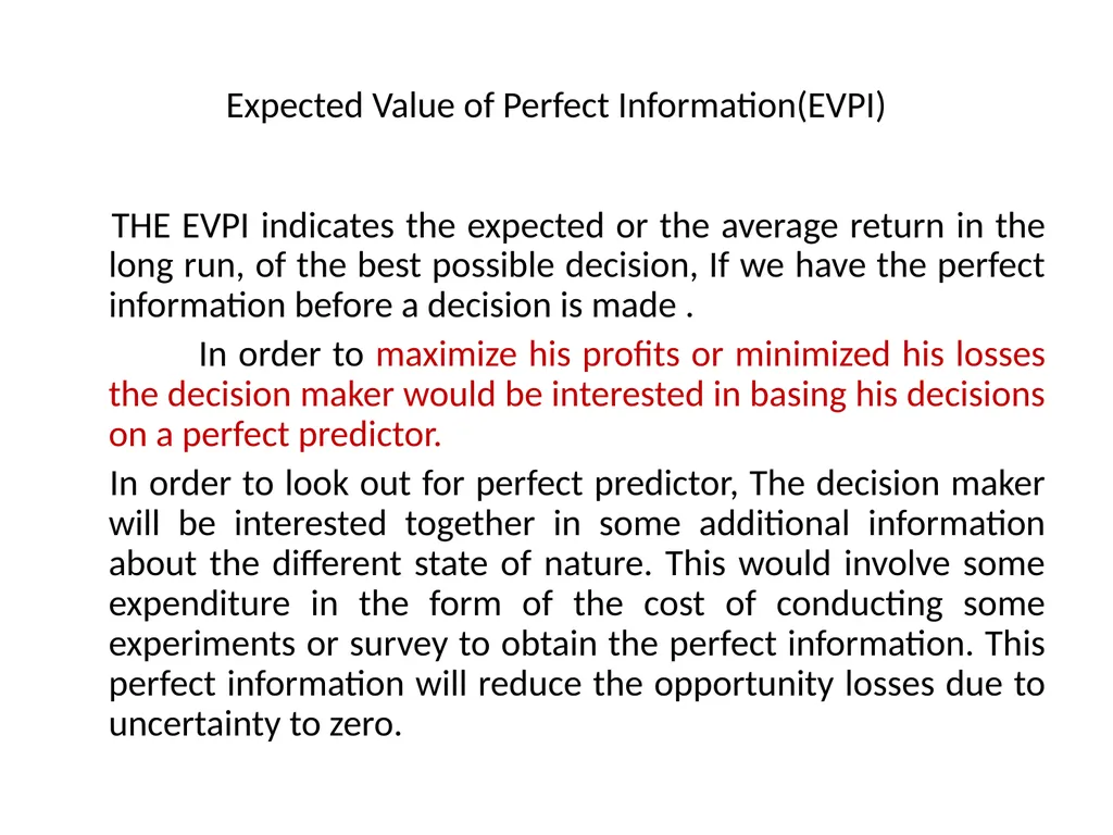
slide47. Expected Value of Perfect Information(EVPI) THE EVPI indicates the expected or the average return in the long run, of the best possible decision, If we have the perfect information before a decision is made .
In order to maximize his profits or minimized his losses the decision maker would be interested in basing his decisions on a perfect predictor.
In order to look out for perfect predictor, The decision maker will be interested together in some additional information about the different state of nature. This would involve some expenditure in the form of the cost of conducting some experiments or survey to obtain the perfect information. This perfect information will reduce the opportunity losses due to uncertainty to zero.<br>
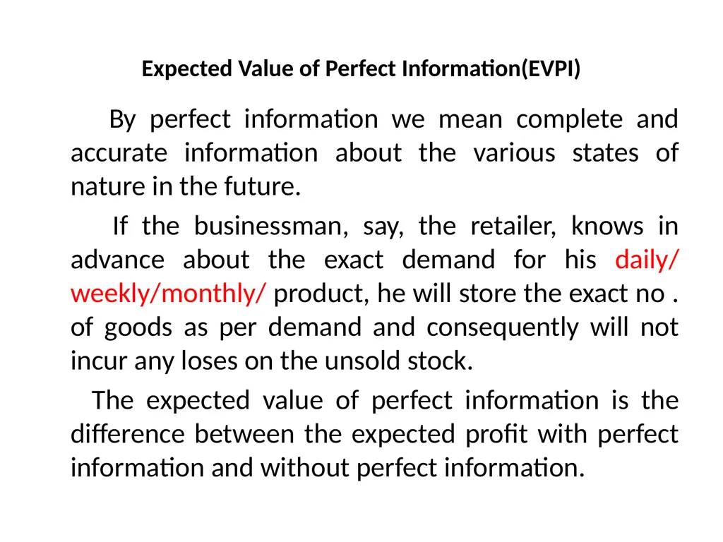
slide48. Expected Value of Perfect Information(EVPI) By perfect information we mean complete and accurate information about the various states of nature in the future.
If the businessman, say, the retailer, knows in advance about the exact demand for his daily/ weekly/monthly/ product, he will store the exact no . of goods as per demand and consequently will not incur any loses on the unsold stock.
The expected value of perfect information is the difference between the expected profit with perfect information and without perfect information.<br>
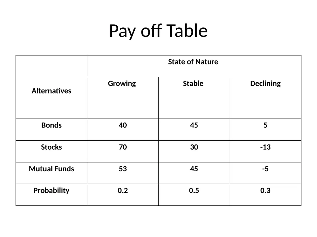
slide49. Pay off Table<br>
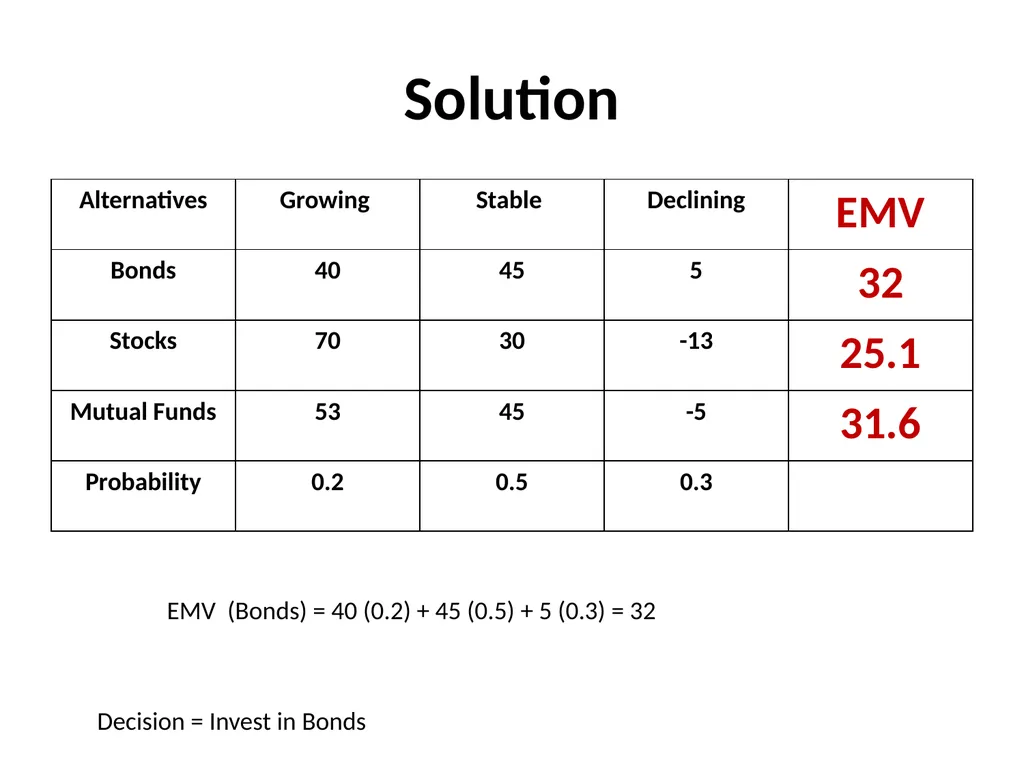
slide50. Solution EMV (Bonds) = 40 (0.2) + 45 (0.5) + 5 (0.3) = 32 Decision = Invest in Bonds<br>
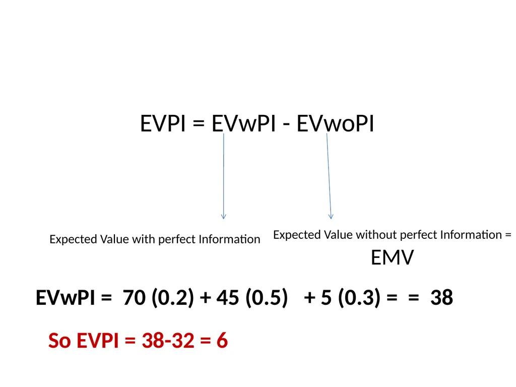
slide51. EVPI = EVwPI - EVwoPI Expected Value without perfect Information =
EMV Expected Value with perfect Information EVwPI = 70 (0.2) + 45 (0.5) + 5 (0.3) = = 38 So EVPI = 38-32 = 6<br>
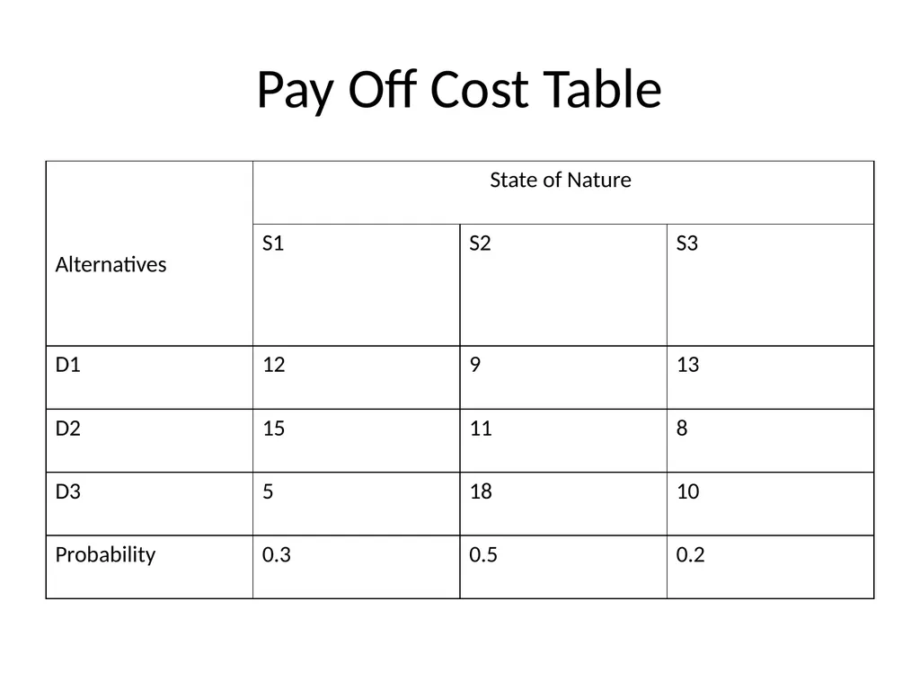
slide52. Pay Off Cost Table<br>
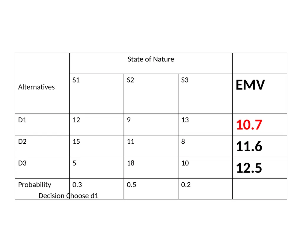
slide53. Decision Choose d1<br>
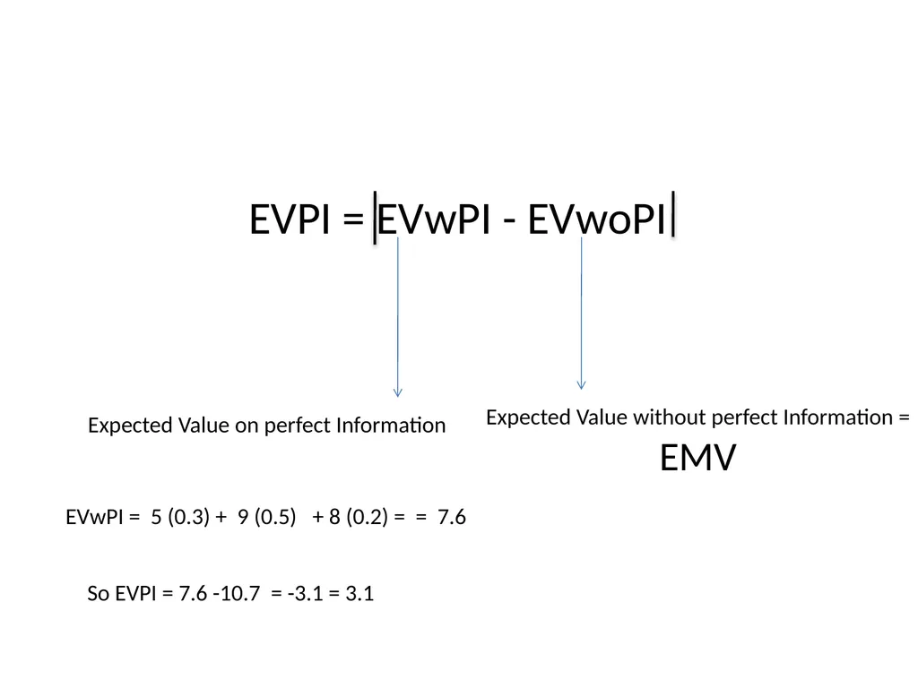
slide54. EVPI = EVwPI - EVwoPI Expected Value without perfect Information =
EMV Expected Value on perfect Information EVwPI = 5 (0.3) + 9 (0.5) + 8 (0.2) = = 7.6 So EVPI = 7.6 -10.7 = -3.1 = 3.1<br>
slide55. Decision Tree<br>
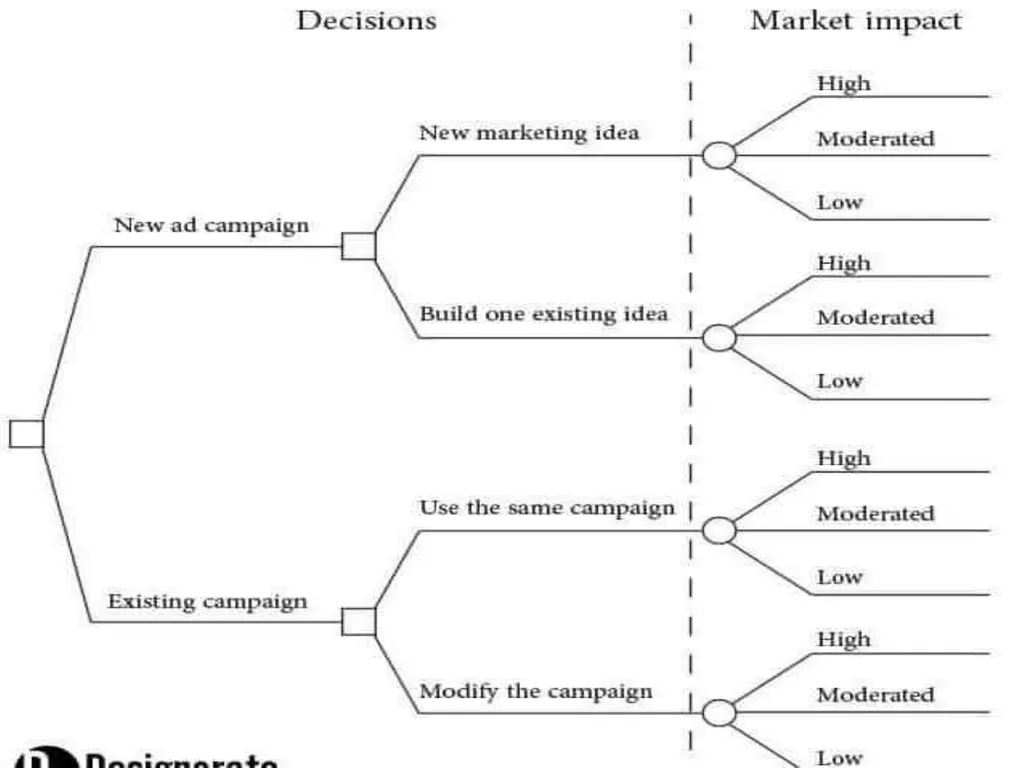
slide56. Definition A decision tree analysis involves the construction of a diagram that shows, at a glance, when decision are expected to be made – in what sequence, their possible consequences and what are the resultant payoff. The result of the computations can be shown directly on the trees.<br>
slide57. Decision Tree A decision tree is made of nodes, branches, probability estimates and payoffs. There are two types of nodes:
Decision nodes
Chance Nodes<br>
slide58. Decision nodes It is represented by a square and represent places where a decision maker must make a decision. Each branch leading away from the node indicates one of the several possible courses of action available to the decision maker.<br>
slide59. Chance Node The Chance node is indicated by a circle and represents a point at which the decision maker will discover the different possible outcomes (state of nature, competitor action etc.).
A branch leading away from a chance node represents the state of nature of a set of chance events.<br>
slide60. Decision Tree Decision Tree depicts decision making under risk, the assumed probabilities of the states of nature are written alongside their respective chance branch.<br>
slide61. Decision Tree The payoff can be positive (revenue or sales) or negative (expenditure or cost) and it can be associated either with decision or chance branches.<br>
slide63. Decision Tree Analysis The optimal sequence of decision in a tree is found by starting at the right hand side and rolling backwards. The aim of this operation is to maximize the return from the decision situation. At each node an expected return is calculated (called positional value. ).
If the node is a chance node, then the position value is calculated as the sum of the products of the probabilities or the branches emanating from the chance node and their respective position values.<br>
slide64. Decision Tree Analysis… If the node is decision node, then the expected return is calculated for each of its branches and the highest return is selected. The procedure continues until the initial node is reached.
The positional values for this node correspond to the maximum expected return obtained from the decision sequence.<br>
slide65. References Operation Research by J K Sharma<br>
by:
Dr. Pravin Kumar Agrawal
Assistant Professor
CSJMU<br>
slide2. Decision-Making Decision-making is needed whenever an individual or an organization (private or public) is faced with a situation of selecting an optimal (or best in view of certain objectives) course of action from among several available alternatives.
For example, an individual may have to decide whether to build a house or to purchase a flat or live in a rented accommodation; whether to join a service or to start own business; which company's car should be purchased, etc. Similarly, a business firm may have to decide the type of technique to be used in production, what is the most appropriate method of advertising its product, etc.
The decision analysis provides certain criteria for the selection of a course of action such that the objective of the decision-maker is satisfied. The course of action selected on the basis of such criteria is termed as the optimal course of action.<br>
slide3. Decision Alternatives Every decision-maker is faced with a set of several alternative courses of action A1, A2, ...... Am and he has to select one of them in view of the objectives to be fulfilled.<br>
slide4. States of Nature These are the future conditions that are not under the control of decision – maker.
A state of nature can be the state of economy (e.g. inflation), a weather condition etc. The state of nature are usually not determined by the action of an individual or an organization, These are the results of an “act of GOD”<br>
slide5. Payoff A numerical value (outcome) resulting from each possible combination of alternatives and state of nature is called pay The payoff values are always conditional values because of unknown states of nature.
Measured within a specified period (e.g. after one year). This period is called as the decision horizon.<br>
slide6. Payoff matrix<br>
slide7. Steps of Decision Making Process Identify and define the Problem.
List all possible future events, called state of nature, which can occur in the context of the decision problem. Such events are not under the control of decision maker because they are erratic in nature.
Identify all the courses of action (alternatives or decision choices) that are available to decision maker. The decision maker has control over these courses of action.
Express the payoffs (pij) resulting from each pair of course of action and state of nature. These payoffs are normally expressed in monetary value.
Apply an appropriate mathematical decision theory model to select the best course of action from the given list on the basis of some criterion (measure of effectiveness) that results in the optimal (desired) payoff.<br>
slide8. Types of Decision Making Environments<br>
slide9. Decision Making under Certainty In this case decision maker has the complete knowledge of consequences of every decision choice (course of action or alternative). Obviously, he will select an alternative that yields the largest return (payoff) for the known future (state of nature).
Eg: the decision to purchase either NSC, KVP, FDs is one in which it is reasonable to assume complete information about the future because there is no doubt that the Indian government will pay the interest when it is due and the principal at maturity<br>
slide10. Decision Making under Risk In this case the decision maker has less than complete knowledge of the consequences of every decision choice (course of action). This is because it is not definitely known which outcome will occur. This means there is one state of nature (future) and for which he makes an assumption of the probability with which each state of nature will occur. Eg product demand high, low, medium.<br>
slide11. Decision Making under Uncertainty A decision problem, where a decision-maker is aware of various possible states of nature but has insufficient information to assign any probabilities of occurrence to them, is termed as decision-making under uncertainty.
A situation of uncertainty arises when there can be more than one possible consequences of selecting any course of action. In terms of the payoff matrix, if the decision-maker selects A1, his payoff can be X11, X12, X13, etc., depending upon which state of nature S1, S2, S3, etc., is going to occur.<br>
slide12. Most significant decisions made in today’s complex environment are formulated under a state of uncertainty. Conditions of uncertainty exist when the future environment is unpredictable. The decision-maker is not aware of all available alternatives, the risks associated with each, and the consequences of each alternative or their probabilities.
The manager does not possess complete information about the alternatives and whatever information is available, may not be completely reliable. In the face of such uncertainty, managers need to make certain assumptions about the situation in order to provide a reasonable framework for decision-making. They have to depend upon their judgment and experience for making decisions.<br>
slide13. Decision making under Uncertainty Optimism (Maximax or Minimin) criterion (2018-19)
Pessimism (Maximin or Minimax) criterion (2018-19)
Equal Probabilities (Laplace) criterion
Coefficeint of optimism (Hurwicz) criterion
Regret (Salvage) criterion<br>
slide14. Optimism (Maximax or Minimin) Criterion In this criterion the decision–maker ensures that he/she should not miss the opportunity to achieve the largest possible profit (maximax) or the lowest possible cost (minimin). Thus he selects the alternative (decision choice or course of action) that represents the maximum of the maxima (or minimum of the minima) payoffs . The working method is as follows:
Locate the maximum (or minimum) payoffs values corresponding to each alternatives (or course of action).
Select an alternative with best anticipated payoff value (maximum for profit and minimum for cost).<br>
slide15. Pessimism (Maximin or Minimax) Criterion In this criterion the decision–maker ensures that he/she would earn no less (or pay no more) than some specified amount. Thus he/she selects the alternative that represents the maximum of the minima (or minimum of the maxima in case of loss) payoffs in case of profits. The working method is as follows:
Locate the minimum (or maximum in case of profit) payoff value in case of loss (or cost) data corresponding to each alternatives.
Select an alternative with the best anticipated payoff value (maximum for profit and minimum for cost).<br>
slide16. Pessimism (Maximin or Minimax) Criterion Since in this criterion the decision-maker is conservative about the future and always anticipates the worst possible outcome (minimum for profit and maximum for cost or loss), it is called a pessimistic decision criterion. This is also known as Wald’s Criterion.<br>
slide17. Equal Probabilities (Laplace) Criterion This criterion is based on, what is known as the principle of insufficient reason. Since the probabilities associated with the occurrence of various events are unknown, there is not enough information to conclude that these probabilities will be different (this is because except in few cases, some information of the likelihood of occurences of states of nature is available). Hence it is assumed that all states of nature will occur with equal probability. That is, each state of nature is assigned an equal probability. As states of nature of mutually exclusive and collectively exhaustive, the probability of each of these must be 1/(number of states of nature)
This criterion involves following steps
Step I Assign equal probabilities 1/(number of states of nature) to each pay off a strategy.
Step II Determine the expected pay off value for each alternative
Step III Select that alternative which corresponds to the maximum (and minimum for cost) of the above expected pay offs.<br>
slide18. Coefficient of Optimism (Hurwicz) Criterion This criterion suggests that a rational decision maker should neither be completely optimistic nor be pessimistic and therefore, must display a mixture of both. Hurwicz, who suggests this criterion, introduced the idea of a coefficient of optimism (denoted by α) to measure the decision maker’s degree of optimism. This coefficient lies between 0 and 1, where 0 represents a completely pessimistic attitude about the future and 1, completely optimistic attitude about the future. Thus, if it is the coefficient of optimism, then (1- α ) will represent the coefficient of pessimism. The working procedure is –<br>
slide19. Hurwicz Formula H (Criterion of Realism) = ᾀ (Maximum in Column) + (1- ᾀ) (Minimum in column) The hurwicz approach suggest that the decision maker must select an alternative that
maximizes<br>
slide20. Coefficient of Optimism (Hurwicz) Criterion Select an alternative with value of H as maximum.
For α=1, the Hurwitz criteria is equal to the maximin or minimax criteria.
For α = 0, it is equal to maximax or minimin criteria.
A difficulty with this criteria is the appropriate selection of α between 0 and 1<br>
slide21. Regret (Salvage) Criterion While the above criterions do not take into account the cost of opportunity loses by making the wrong decision, the Savage criterion does so. The savage criterion is based on the concept of regret (or opportunity loss) and calls for selecting the course of action that minimizes the maximum regret. This criterion is assume that decision maker feels regret after adopting a wrong course of action (alternative) resulting in an opportunity loss of pay off. The working method is as follows:<br>
slide22. Regret (Salvage) Criterion Step I From the given pay off matrix, develop an opportunity loss (or regret) matrix as follows
(a) Find the best pay off corresponding to each state of nature.
(b) Subtract all other entries (payoff values) in that row from this value.
Step II: For each course of action (Strategy or alternative) identify the worst or maximum regret value. Record this number in a new row.
Step III: Select the course of action (alternative) with the smallest anticipated opportunity – loss value<br>
slide23. Numerical A food Product company is contemplating the introduction of a revolutionary new product with new packaging or replacing the existing product at much higher price (S1). It may even make a moderate change in the composition of existing product, with a new packaging at a small increase in price (S2), or may a small change in the composition of the existing product, backing it with the word new and the negligible increase in price (S3). The three possible state of Nature or events are:
(i) High increase in Sale N1
(ii) No Change in Sale N2
(iii) decrese in Sale N3.<br>
slide24. The marketing department of the company worked out the payoffs in terms of yearly net profits for each of the strategies of three events (expected sales). This is represented in the following table:<br>
slide25. Which Strategy Should be concerned executive choose on the basis of: Maximin Criterion
Maximax Criterion
Minimax Regret Criterion
Laplace Criterion<br>
slide26. Numerical Which Strategy Should be concerned executive choose on the basis of: Maximin Criterion
Maximax Criterion
Minimax Regret Criterion
Laplace Criterion<br>
slide27. (a) Maximin Criterian The maximum of column minima is 3,00,000 . Hence the company should adopt
Strategy S3<br>
slide28. (a) Maximax Criterian The maximum of column maxima is 7,00,000 . Hence the company should adopt
Strategy S1.<br>
slide29. Minimax Regret Criterion<br>
slide30. Minimax Regret Criterion Hence the company should adopt minimum opportunity loss Strategy S1. Minimax Regret<br>
slide31. Laplace Criterion Since we do not know the probabilities of State of nature, assume that they are equal. In this example we assume that each state of nature has a probability of 1/3 occurrence. Thus<br>
slide32. Minimax Regret Criterion<br>
slide33. Minimax Regret Criterion Since the largest expected return is from strategy S1, the executive must select strategy S1.<br>
slide34. Decision Making Under Risk A probabilistic decision situation in which more than one state of nature exists and the decision maker has sufficient information to assign probability values to the likely occurrences of each of these states.
The best decision is to select that course of action which has the largest expected pay off value.
The expected (average) payoff of an alternative is sum of all possible payoffs of that alternative, weighted by the probabilities of the occurrence of those payoffs.
The most widely used criterion for evaluating various course of action (alternatives) under risk is the Expected Monetary Value (EMV).<br>
slide35. Expected Monetary Value (EMV) (2018-19) The expected monetary value (EMV) for a given course of action is the weighted sum of possible payoffs for each alternative. The expected (or mean) value is the long run average value that would result of the decision were repeated a large no. of times. Mathematically EMV is stated as follows:
EMV = Ʃ pijpj
Where,
m = no. of possible state of nature
pi = Probability of occurrence of state of nature, Ni
pij = payoff associated with state of nature Ni and course of action Sj.<br>
slide36. Expected Monetary Value Example I You are managing a software development project and identified a risk related to market demand. The possibility of risk is 20% and if it occurs you will lose Rs. 10,000. Now we will calculate the EMV of this risk.<br>
slide37. Example I Probability of occurrence: 20%
Impact of risk : Rs. – 10,000
EMV = 0.2 x -10,000 = Rs. – 2,000<br>
slide38. Expected Monetary Value Example II You are managing an IT project and identified a risk related to customer’s demand. However, you also identified an opportunity which increases the sales price. The possibility of risk is 10% and if it occurs you will lose 50,000 USD, on the other hand, the possibility of opportunity is 15% and if it occurs you gain 30,000 USD. Now we will calculate the EMV of this situation.<br>
slide39. I Case
Probability of occurrence : 10%
Impact of risk : – 50,000 USD
EMV = 0.1 x -50,000 = – 5,000 USD
II Case
Probability of occurrence: 15%
Impact of risk : 30,000 USD
EMV = 0.15 x 30,000 = 4,500 USD
The Expected Monetary Value of this situation is – 5,000 USD + 4,500 USD = 500 USD<br>
slide40. Suppose you are a project manager of a pipeline project and your project have some risks that may cause delay and cost overruns.
Project Risk 1: There is a 25% possibility of heavy rain. This will cause a delay in the project for 3 weeks and cost Rs. 100,000.
Project Risk 2: There is a 15% percent probability of the price of rental equipment increasing, which will cost Rs. 200,000.
Project Risk 3: There is a 10% percent probability of the price of labor increases, which will cost Rs. 90,000.
Project Risk 4: There is a 30% possibility of increasing the productivity of excavators due to the ground conditions. This will enable to complete the project 2 weeks before and save Rs. 50,000.<br>
slide41. Now Let’s calculate the EMV of the project In this scenario, the project manager should add Rs. 49,000 to the project budget to
manage those risks.<br>
slide42. Benefits of Expected Monetary Value (EMV) Analysis Enables to calculate contingency reserve.
Improves statistical thinking
Improves decision making
This technique gives realistic results when there is a large number of risks in the project.
Helps to select the risk management alternative which requires less cost.
This technique does not require additional cost, it only requires an expert to make risk calculations.
It can be used in conjunction with decision tree analysis.<br>
slide43. Limitations of Expected Monetary Value (EMV) Analysis Although the EMV is a useful technique to perform a quantitative risk analysis, it has some limitations.
If the positive and negative risks are not identified properly, the result would be misleading.
The impact of risk calculation as a monetary value may be difficult in some cases.<br>
slide44. Expected Opportunity Loss One more way of maximizing monitory value is to minimize the expected opportunity loss or expected value of regret. The conditional EOL or regret function for a particular course of action is determined by taking the difference between payoff value of the most favorable course of action i.e. maximum pay off and pay off for each Course of action for a given state of nature. The course of action for which EOL is minimum is recommended.
EOL = Ʃ lij pi
lij = opportunity loss due to state of nature Ni and Course of Action Sj
Pi = Probability of occurrences of state of nature, Ni<br>
slide45. https://www.coursehero.com/file/p2losa4/Decision-Making-under-Risk-Expected-Opportunity-Loss-EOL-Another-useful-way-of/<br>
slide46. Expected Value of Perfect Information(EVPI) EVPI is the maximum amount which the decision maker can spend to obtain the perfect information on which to base a given decision is called expected value of perfect information.
EVPI = Expected Profit with perfect information[EPPI]
– Expected Monetary value<br>
slide47. Expected Value of Perfect Information(EVPI) THE EVPI indicates the expected or the average return in the long run, of the best possible decision, If we have the perfect information before a decision is made .
In order to maximize his profits or minimized his losses the decision maker would be interested in basing his decisions on a perfect predictor.
In order to look out for perfect predictor, The decision maker will be interested together in some additional information about the different state of nature. This would involve some expenditure in the form of the cost of conducting some experiments or survey to obtain the perfect information. This perfect information will reduce the opportunity losses due to uncertainty to zero.<br>
slide48. Expected Value of Perfect Information(EVPI) By perfect information we mean complete and accurate information about the various states of nature in the future.
If the businessman, say, the retailer, knows in advance about the exact demand for his daily/ weekly/monthly/ product, he will store the exact no . of goods as per demand and consequently will not incur any loses on the unsold stock.
The expected value of perfect information is the difference between the expected profit with perfect information and without perfect information.<br>
slide49. Pay off Table<br>
slide50. Solution EMV (Bonds) = 40 (0.2) + 45 (0.5) + 5 (0.3) = 32 Decision = Invest in Bonds<br>
slide51. EVPI = EVwPI - EVwoPI Expected Value without perfect Information =
EMV Expected Value with perfect Information EVwPI = 70 (0.2) + 45 (0.5) + 5 (0.3) = = 38 So EVPI = 38-32 = 6<br>
slide52. Pay Off Cost Table<br>
slide53. Decision Choose d1<br>
slide54. EVPI = EVwPI - EVwoPI Expected Value without perfect Information =
EMV Expected Value on perfect Information EVwPI = 5 (0.3) + 9 (0.5) + 8 (0.2) = = 7.6 So EVPI = 7.6 -10.7 = -3.1 = 3.1<br>
slide55. Decision Tree<br>
slide56. Definition A decision tree analysis involves the construction of a diagram that shows, at a glance, when decision are expected to be made – in what sequence, their possible consequences and what are the resultant payoff. The result of the computations can be shown directly on the trees.<br>
slide57. Decision Tree A decision tree is made of nodes, branches, probability estimates and payoffs. There are two types of nodes:
Decision nodes
Chance Nodes<br>
slide58. Decision nodes It is represented by a square and represent places where a decision maker must make a decision. Each branch leading away from the node indicates one of the several possible courses of action available to the decision maker.<br>
slide59. Chance Node The Chance node is indicated by a circle and represents a point at which the decision maker will discover the different possible outcomes (state of nature, competitor action etc.).
A branch leading away from a chance node represents the state of nature of a set of chance events.<br>
slide60. Decision Tree Decision Tree depicts decision making under risk, the assumed probabilities of the states of nature are written alongside their respective chance branch.<br>
slide61. Decision Tree The payoff can be positive (revenue or sales) or negative (expenditure or cost) and it can be associated either with decision or chance branches.<br>
slide63. Decision Tree Analysis The optimal sequence of decision in a tree is found by starting at the right hand side and rolling backwards. The aim of this operation is to maximize the return from the decision situation. At each node an expected return is calculated (called positional value. ).
If the node is a chance node, then the position value is calculated as the sum of the products of the probabilities or the branches emanating from the chance node and their respective position values.<br>
slide64. Decision Tree Analysis… If the node is decision node, then the expected return is calculated for each of its branches and the highest return is selected. The procedure continues until the initial node is reached.
The positional values for this node correspond to the maximum expected return obtained from the decision sequence.<br>
slide65. References Operation Research by J K Sharma<br>