04
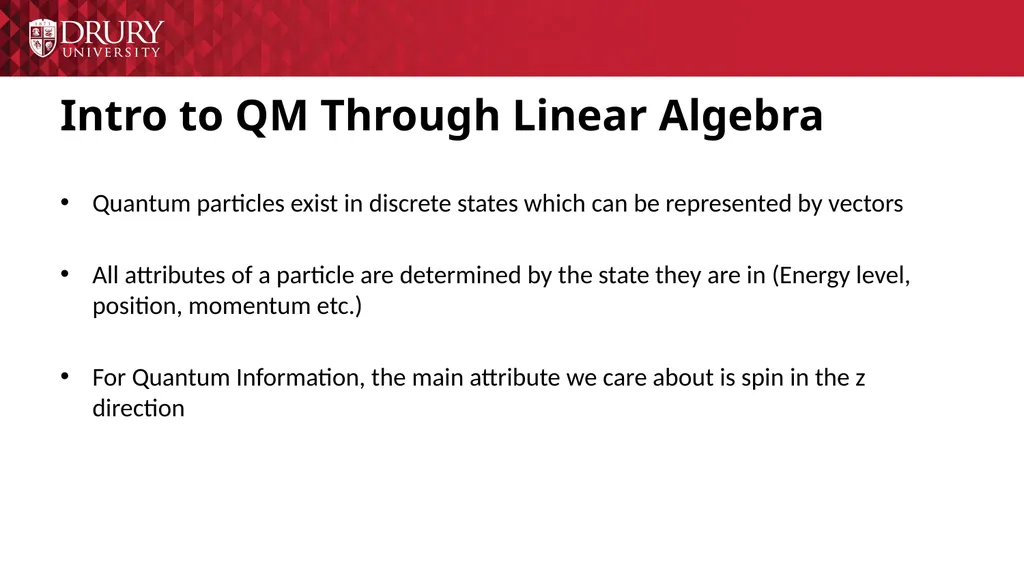
In Quantum Mechanics, our vectors are complex, and all lie in L2 (-∞,∞) (Hilbert Space)
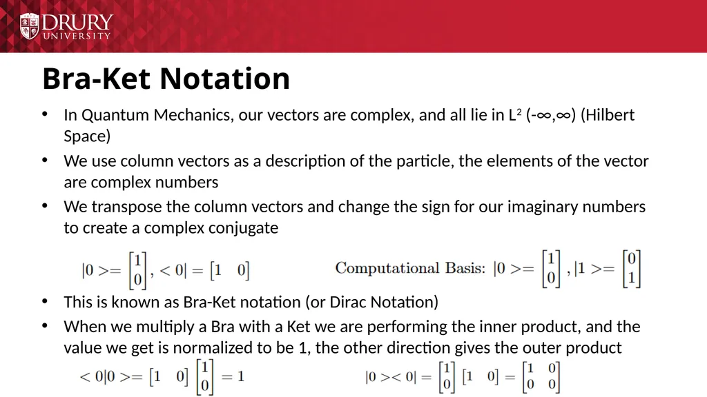
We use column vectors as a description of the particle, the elements of the vector are complex numbers
We transpose the column vectors and change the sign for our imaginary numbers to create a complex conjugate
This is known as Bra-Ket notation (or Dirac Notation)
When we multiply a Bra with a Ket we are performing the inner product, and the value we get is normalized to be 1, the other direction gives the outer product Bra-Ket Notation<br>
05
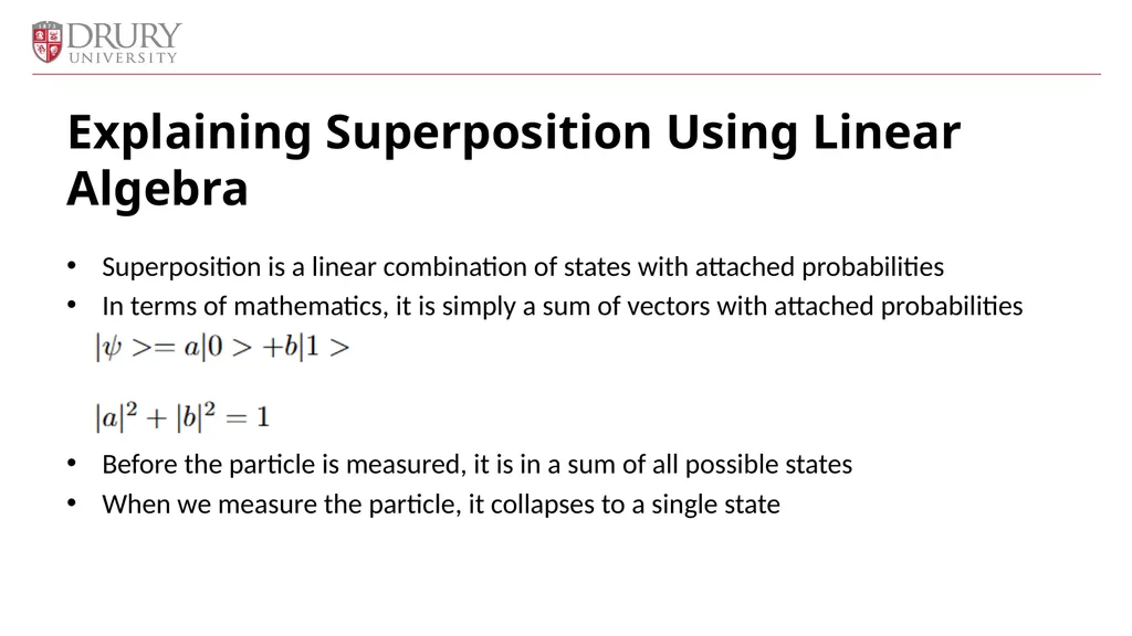
Superposition is a linear combination of states with attached probabilities
In terms of mathematics, it is simply a sum of vectors with attached probabilities
Before the particle is measured, it is in a sum of all possible states
When we measure the particle, it collapses to a single state Explaining Superposition Using Linear Algebra<br>
06
In Quantum Information Theory the main aspect of a particle we focus on is its spin in the z direction
For particles such as electrons, they only have 2 spin states, spin up or spin down ½
This is convenient because of how it parallels a classical bit, which has two different possible values, 0 or 1
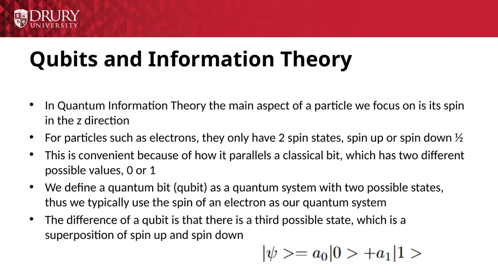
We define a quantum bit (qubit) as a quantum system with two possible states, thus we typically use the spin of an electron as our quantum system
The difference of a qubit is that there is a third possible state, which is a superposition of spin up and spin down Qubits and Information Theory<br>
07
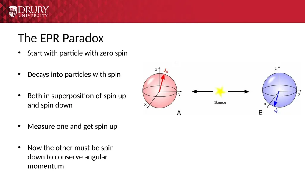
Start with particle with zero spin
Decays into particles with spin
Both in superposition of spin up and spin down
Measure one and get spin up
Now the other must be spin down to conserve angular momentum The EPR Paradox<br>
08
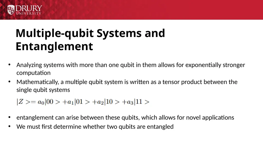
Analyzing systems with more than one qubit in them allows for exponentially stronger computation
Mathematically, a multiple qubit system is written as a tensor product between the single qubit systems
entanglement can arise between these qubits, which allows for novel applications
We must first determine whether two qubits are entangled Multiple-qubit Systems and Entanglement<br>
09
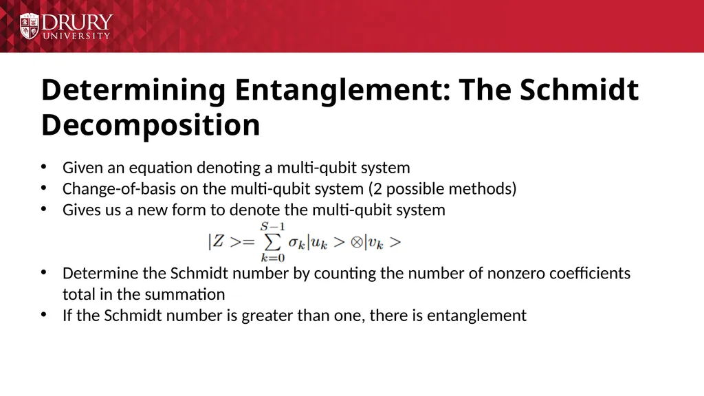
Determining Entanglement: The Schmidt Decomposition Given an equation denoting a multi-qubit system
Change-of-basis on the multi-qubit system (2 possible methods)
Gives us a new form to denote the multi-qubit system
Determine the Schmidt number by counting the number of nonzero coefficients total in the summation
If the Schmidt number is greater than one, there is entanglement<br>
10
Conceptual Explanation of The Schmidt Decomposition The Schmidt decomposition analyzes a vector space that is a tensor product of two separate subspaces
The newly constructed equation dictates how many axis the two subspaces share
All subspaces will share at least one axis with each other
If more than one axis is shared, it means that the two subspaces are entangled with each other, since an output in one subspace will dictate the output in the other<br>
11
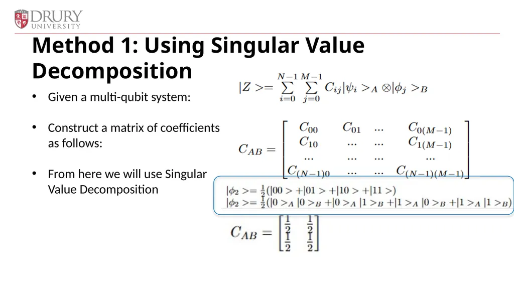
Method 1: Using Singular Value Decomposition Given a multi-qubit system:
Construct a matrix of coefficients as follows:
From here we will use Singular Value Decomposition<br>
12
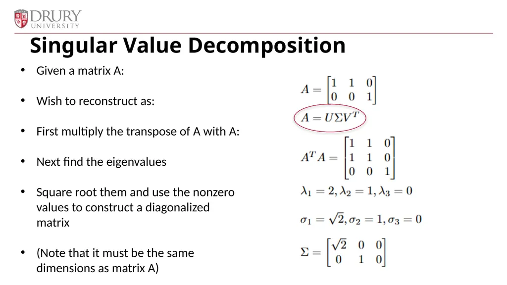
Singular Value Decomposition Given a matrix A:
Wish to reconstruct as:
First multiply the transpose of A with A:
Next find the eigenvalues
Square root them and use the nonzero values to construct a diagonalized matrix
(Note that it must be the same dimensions as matrix A)<br>
13
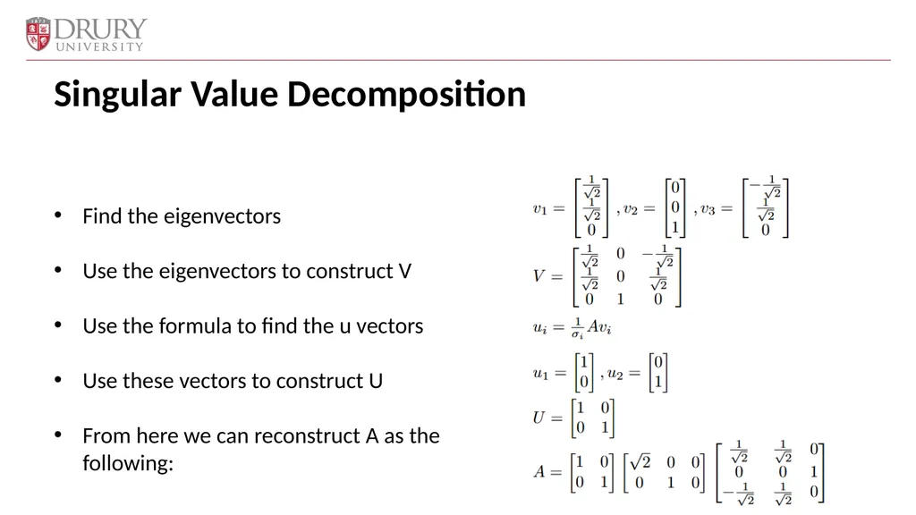
Find the eigenvectors
Use the eigenvectors to construct V
Use the formula to find the u vectors
Use these vectors to construct U
From here we can reconstruct A as the following: Singular Value Decomposition<br>
14
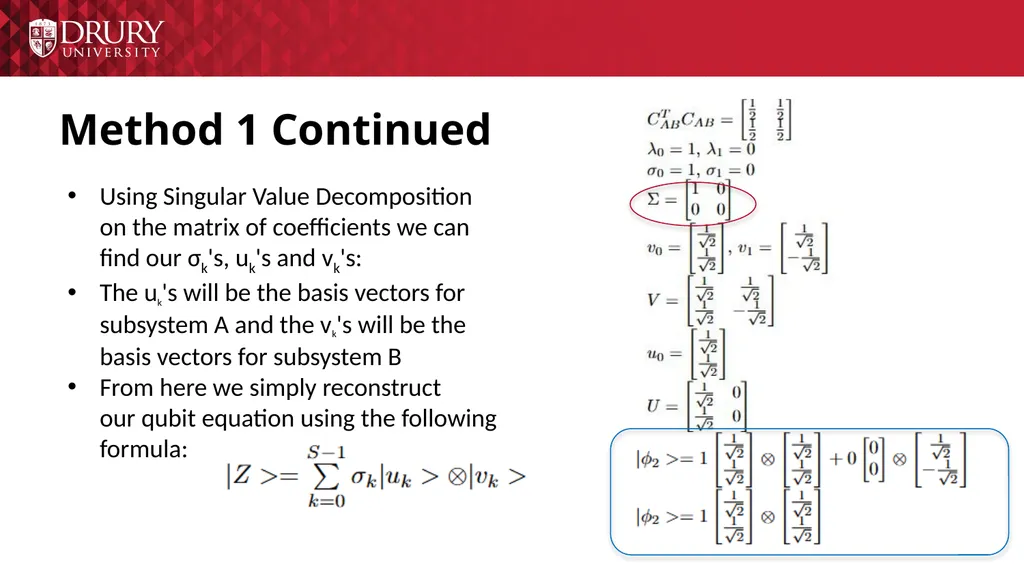
Method 1 Continued Using Singular Value Decomposition on the matrix of coefficients we can find our σk's, uk's and vk's:
The uk's will be the basis vectors for subsystem A and the vk's will be the basis vectors for subsystem B
From here we simply reconstruct our qubit equation using the following formula:<br>
15
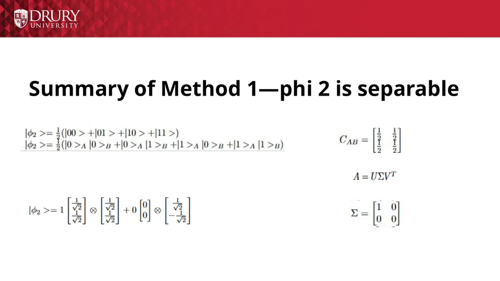
Summary of Method 1—phi 2 is separable<br>
16
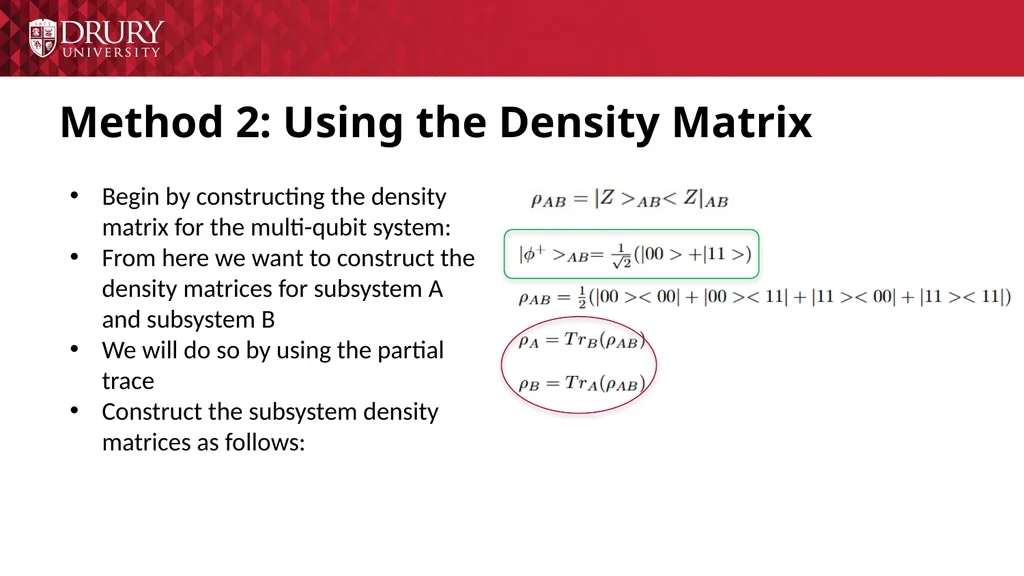
Method 2: Using the Density Matrix Begin by constructing the density matrix for the multi-qubit system:
From here we want to construct the density matrices for subsystem A and subsystem B
We will do so by using the partial trace
Construct the subsystem density matrices as follows:<br>
17
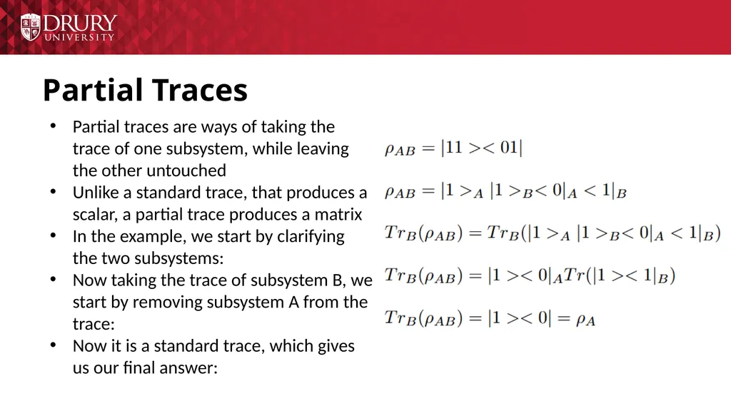
Partial Traces Partial traces are ways of taking the trace of one subsystem, while leaving the other untouched
Unlike a standard trace, that produces a scalar, a partial trace produces a matrix
In the example, we start by clarifying the two subsystems:
Now taking the trace of subsystem B, we start by removing subsystem A from the trace:
Now it is a standard trace, which gives us our final answer:<br>
18
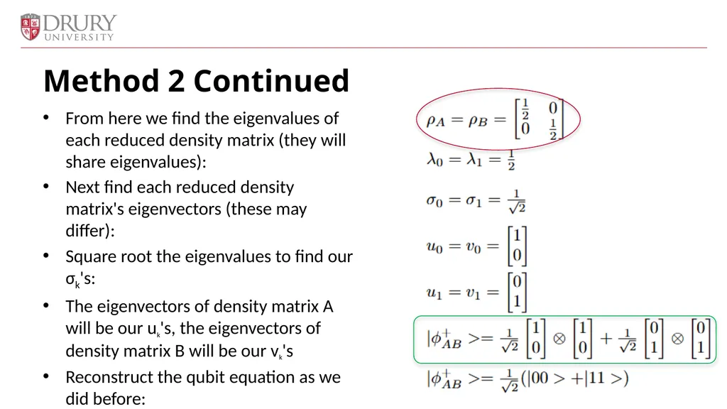
From here we find the eigenvalues of each reduced density matrix (they will share eigenvalues):
Next find each reduced density matrix's eigenvectors (these may differ):
Square root the eigenvalues to find our σk's:
The eigenvectors of density matrix A will be our uk's, the eigenvectors of density matrix B will be our vk's
Reconstruct the qubit equation as we did before: Method 2 Continued<br>
19
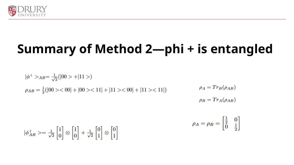
Summary of Method 2—phi + is entangled<br>
20
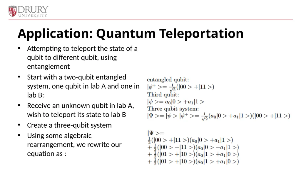
Attempting to teleport the state of a qubit to different qubit, using entanglement
Start with a two-qubit entangled system, one qubit in lab A and one in lab B:
Receive an unknown qubit in lab A, wish to teleport its state to lab B
Create a three-qubit system
Using some algebraic rearrangement, we rewrite our equation as : Application: Quantum Teleportation<br>
21
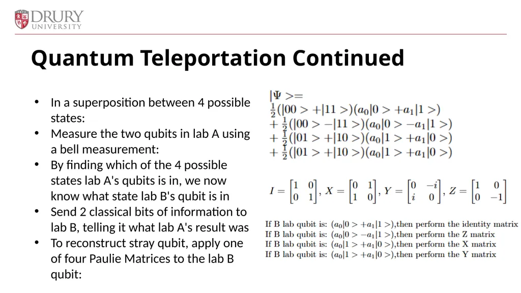
Quantum Teleportation Continued In a superposition between 4 possible states:
Measure the two qubits in lab A using a bell measurement:
By finding which of the 4 possible states lab A's qubits is in, we now know what state lab B's qubit is in
Send 2 classical bits of information to lab B, telling it what lab A's result was
To reconstruct stray qubit, apply one of four Paulie Matrices to the lab B qubit:<br>
22
Investigate the connection between the two Schmidt Decomposition methods
Determine correlation between reduced density matrices and maximal entanglement Future work<br>
23
Bradley, T. D. (2020). At the interface of algebra and statistics (Doctoral dissertation, City University of New York).
Cavalcanti, E. G., Drummond, P. D., Bachor, H. A., & Reid, M. D. (2009). Spin entanglement, decoherence and Bohm’s EPR paradox. Optics Express, 17(21), 18693-18702.
Griffiths, D. J., & Schroeter, D. F. (2018). Introduction to quantum mechanics. Cambridge university press.
Jaeger, G. (2007). Quantum information (pp. 81-89). Springer New York. Works Cited<br>
24
Thank you! lboswell@drury.edu<br>