
Valuation: Packet 3 Real Options, Acquisition
PM
Published · 159 slides · 0 views

1 / 1







Description
Valuation: Packet 3 Real Options, Acquisition Valuation and Value Enhancement Updated: January 2025 Aswath Damodaran 1 Real Options: Fact and Fantasy Aswath Damodaran 2 Underlying Theme: Searching for an Elusive Premium Traditional
Related Topics
Share
Embed code
Download this presentation From Below
"Valuation: Packet 3 Real Options, Acquisition" is the property of its rightful owner. Permission is granted to download and print the materials on this website for personal, non-commercial use only, and to display it on your personal computer provided you do not modify the materials and that you retain all copyright notices contained in the materials. By downloading content from our website, you accept the terms of this agreement.
Presentation Transcript
01
Valuation: Packet 3
Real Options, Acquisition Valuation and Value Enhancement Updated: January 2025 Aswath Damodaran 1<br>
02
Real Options: Fact and Fantasy Aswath Damodaran 2<br>
03
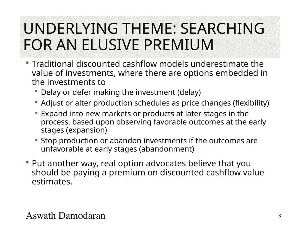
Underlying Theme: Searching for an Elusive Premium Traditional discounted cashflow models underestimate the value of investments, where there are options embedded in the investments to
Delay or defer making the investment (delay)
Adjust or alter production schedules as price changes (flexibility)
Expand into new markets or products at later stages in the process, based upon observing favorable outcomes at the early stages (expansion)
Stop production or abandon investments if the outcomes are unfavorable at early stages (abandonment)
Put another way, real option advocates believe that you should be paying a premium on discounted cashflow value estimates. Aswath Damodaran 3<br>
Delay or defer making the investment (delay)
Adjust or alter production schedules as price changes (flexibility)
Expand into new markets or products at later stages in the process, based upon observing favorable outcomes at the early stages (expansion)
Stop production or abandon investments if the outcomes are unfavorable at early stages (abandonment)
Put another way, real option advocates believe that you should be paying a premium on discounted cashflow value estimates. Aswath Damodaran 3<br>
04
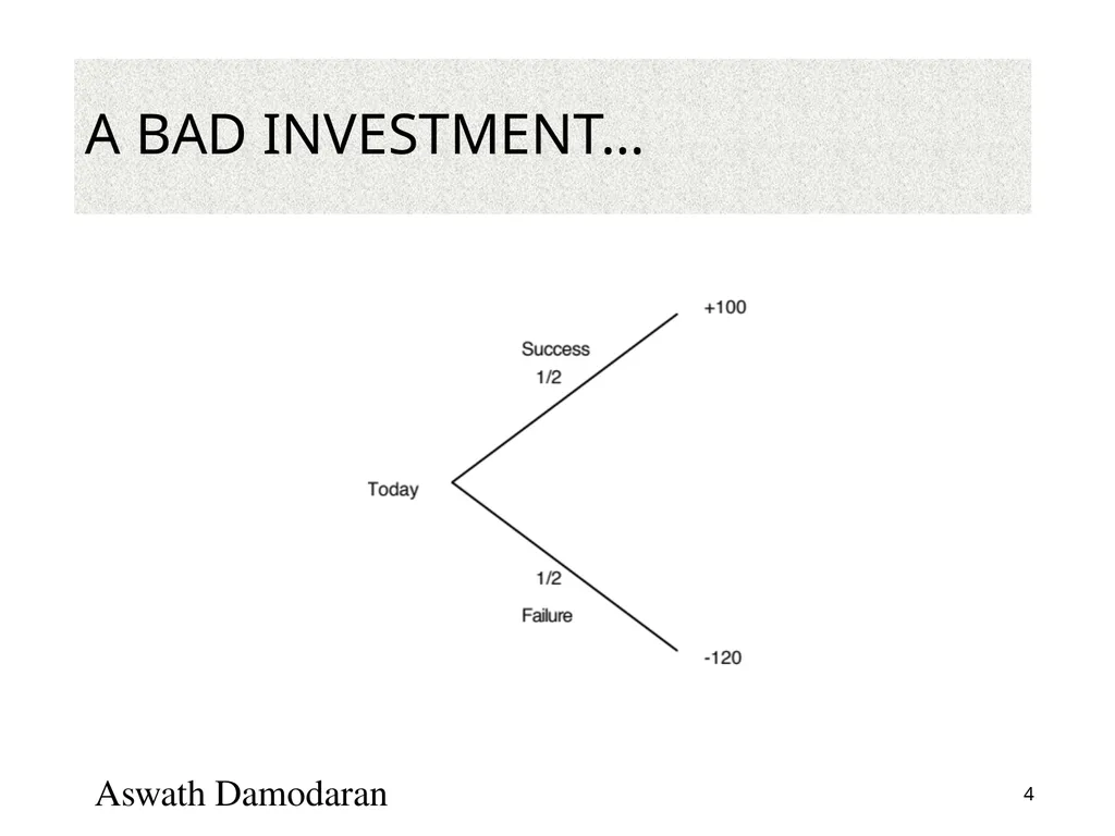
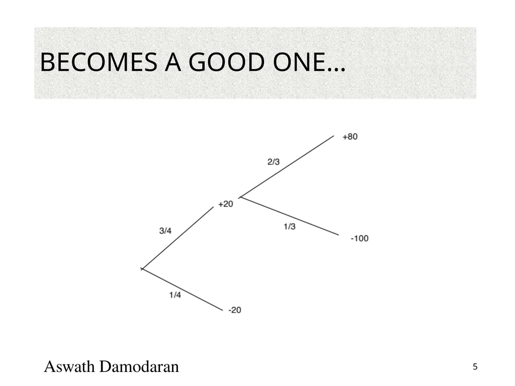
A bad investment… Aswath Damodaran 4<br>
05
Becomes a good one… Aswath Damodaran 5<br>
06
Three Basic Questions When is there a real option embedded in a decision or an asset?
When does that real option have significant economic value?
Can that value be estimated using an option pricing model? Aswath Damodaran 6<br>
When does that real option have significant economic value?
Can that value be estimated using an option pricing model? Aswath Damodaran 6<br>
07
When is there an option embedded in an action? An option provides the holder with the right to buy or sell a specified quantity of an underlying asset at a fixed price (called a strike price or an exercise price) at or before the expiration date of the option.
There has to be a clearly defined underlying asset whose value changes over time in unpredictable ways.
The payoffs on this asset (real option) have to be contingent on a specified event occurring within a finite period. Aswath Damodaran 7<br>
There has to be a clearly defined underlying asset whose value changes over time in unpredictable ways.
The payoffs on this asset (real option) have to be contingent on a specified event occurring within a finite period. Aswath Damodaran 7<br>
08
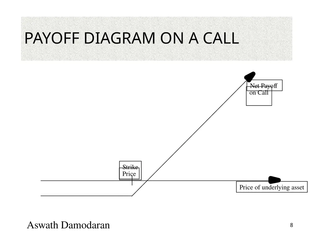
Payoff Diagram on a Call Aswath Damodaran 8 Price of underlying asset Strike Price Net Payoff on Call<br>
09
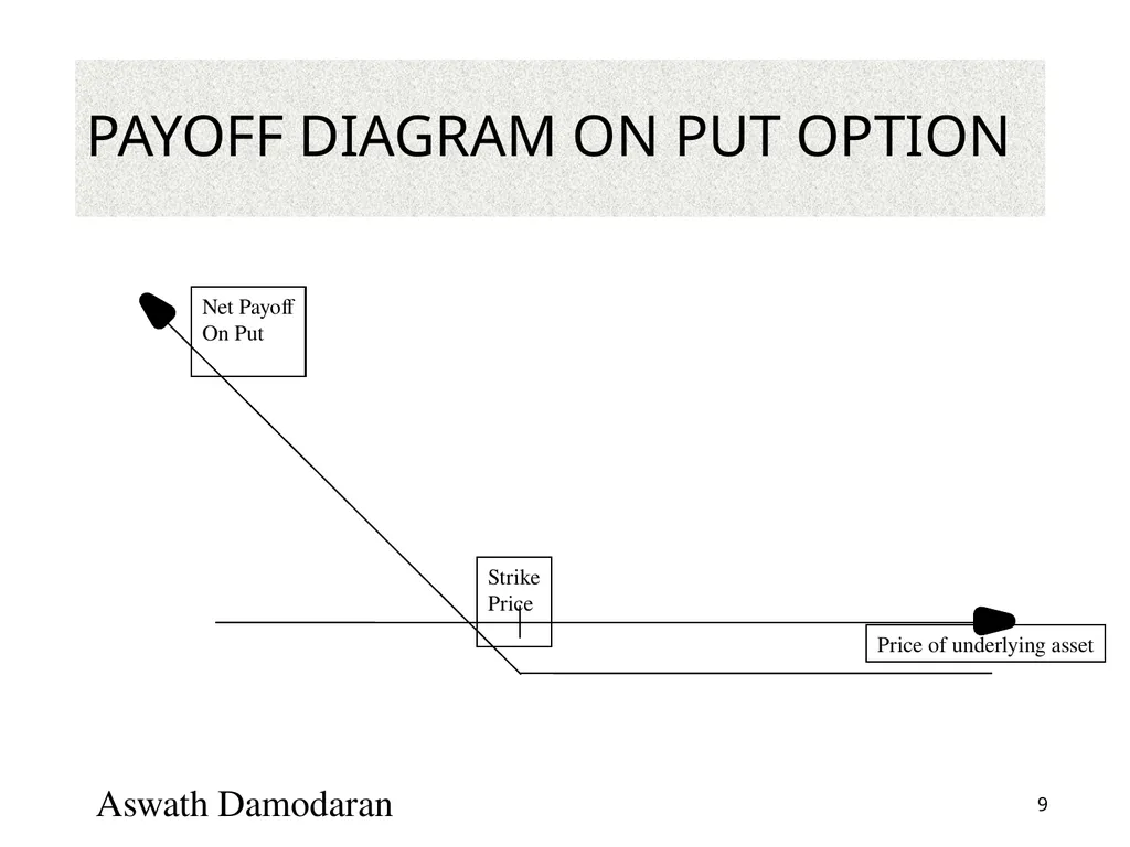
Payoff Diagram on Put Option Aswath Damodaran 9 Price of underlying asset Strike
Price Net Payoff
On Put<br>
Price Net Payoff
On Put<br>
10
When does the option have significant economic value? For an option to have significant economic value, there has to be a restriction on competition in the event of the contingency. In a perfectly competitive product market, no contingency, no matter how positive, will generate positive net present value.
At the limit, real options are most valuable when you have exclusivity - you and only you can take advantage of the contingency. They become less valuable as the barriers to competition become less steep. Aswath Damodaran 10<br>
At the limit, real options are most valuable when you have exclusivity - you and only you can take advantage of the contingency. They become less valuable as the barriers to competition become less steep. Aswath Damodaran 10<br>
11
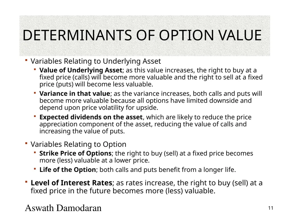
Determinants of option value Variables Relating to Underlying Asset
Value of Underlying Asset; as this value increases, the right to buy at a fixed price (calls) will become more valuable and the right to sell at a fixed price (puts) will become less valuable.
Variance in that value; as the variance increases, both calls and puts will become more valuable because all options have limited downside and depend upon price volatility for upside.
Expected dividends on the asset, which are likely to reduce the price appreciation component of the asset, reducing the value of calls and increasing the value of puts.
Variables Relating to Option
Strike Price of Options; the right to buy (sell) at a fixed price becomes more (less) valuable at a lower price.
Life of the Option; both calls and puts benefit from a longer life.
Level of Interest Rates; as rates increase, the right to buy (sell) at a fixed price in the future becomes more (less) valuable. Aswath Damodaran 11<br>
Value of Underlying Asset; as this value increases, the right to buy at a fixed price (calls) will become more valuable and the right to sell at a fixed price (puts) will become less valuable.
Variance in that value; as the variance increases, both calls and puts will become more valuable because all options have limited downside and depend upon price volatility for upside.
Expected dividends on the asset, which are likely to reduce the price appreciation component of the asset, reducing the value of calls and increasing the value of puts.
Variables Relating to Option
Strike Price of Options; the right to buy (sell) at a fixed price becomes more (less) valuable at a lower price.
Life of the Option; both calls and puts benefit from a longer life.
Level of Interest Rates; as rates increase, the right to buy (sell) at a fixed price in the future becomes more (less) valuable. Aswath Damodaran 11<br>
12
When can you use option pricing models to value real options? The notion of a replicating portfolio that drives option pricing models makes them most suited for valuing real options where
The underlying asset is traded - this yield not only observable prices and volatility as inputs to option pricing models but allows for the possibility of creating replicating portfolios
An active marketplace exists for the option itself.
The cost of exercising the option is known with some degree of certainty.
When option pricing models are used to value real assets, we have to accept the fact that
The value estimates that emerge will be far more imprecise.
The value can deviate much more dramatically from market price because of the difficulty of arbitrage. Aswath Damodaran 12<br>
The underlying asset is traded - this yield not only observable prices and volatility as inputs to option pricing models but allows for the possibility of creating replicating portfolios
An active marketplace exists for the option itself.
The cost of exercising the option is known with some degree of certainty.
When option pricing models are used to value real assets, we have to accept the fact that
The value estimates that emerge will be far more imprecise.
The value can deviate much more dramatically from market price because of the difficulty of arbitrage. Aswath Damodaran 12<br>
13
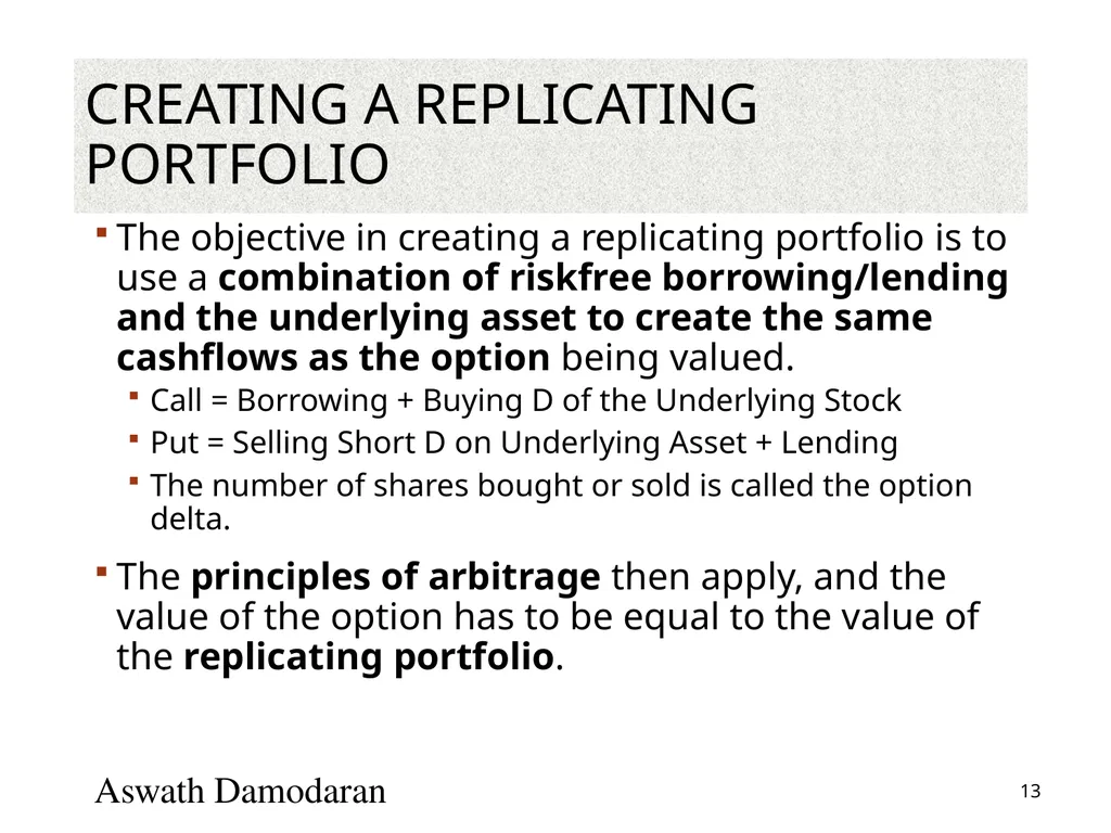
Creating a replicating portfolio The objective in creating a replicating portfolio is to use a combination of riskfree borrowing/lending and the underlying asset to create the same cashflows as the option being valued.
Call = Borrowing + Buying D of the Underlying Stock
Put = Selling Short D on Underlying Asset + Lending
The number of shares bought or sold is called the option delta.
The principles of arbitrage then apply, and the value of the option has to be equal to the value of the replicating portfolio. Aswath Damodaran 13<br>
Call = Borrowing + Buying D of the Underlying Stock
Put = Selling Short D on Underlying Asset + Lending
The number of shares bought or sold is called the option delta.
The principles of arbitrage then apply, and the value of the option has to be equal to the value of the replicating portfolio. Aswath Damodaran 13<br>
14
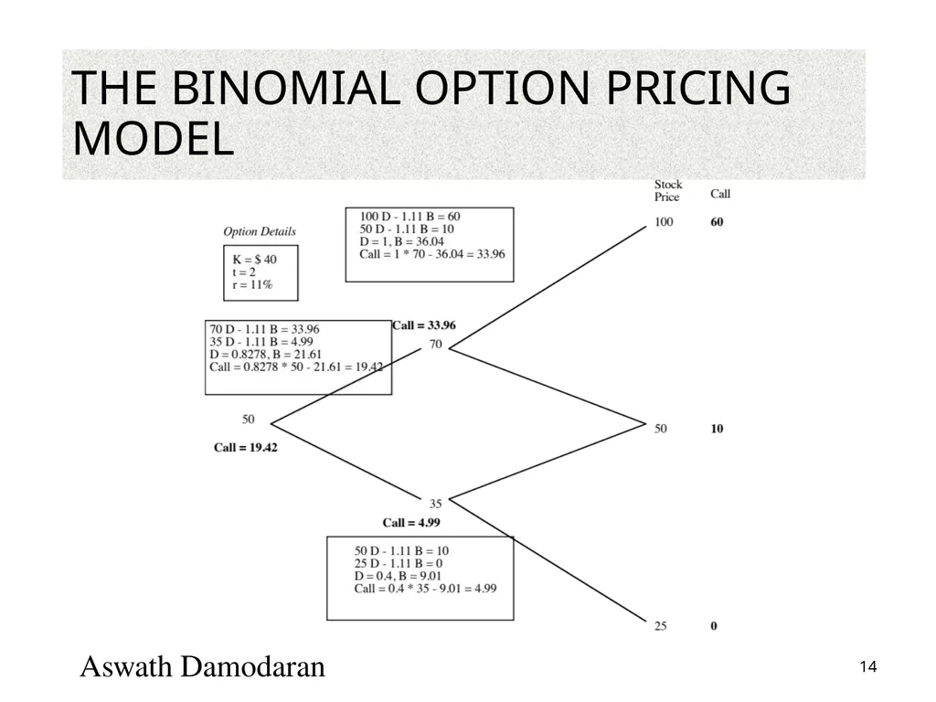
The Binomial Option Pricing Model Aswath Damodaran 14<br>
15
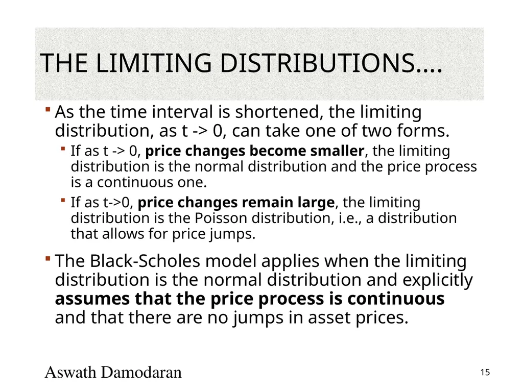
The Limiting Distributions…. As the time interval is shortened, the limiting distribution, as t -> 0, can take one of two forms.
If as t -> 0, price changes become smaller, the limiting distribution is the normal distribution and the price process is a continuous one.
If as t->0, price changes remain large, the limiting distribution is the Poisson distribution, i.e., a distribution that allows for price jumps.
The Black-Scholes model applies when the limiting distribution is the normal distribution and explicitly assumes that the price process is continuous and that there are no jumps in asset prices. Aswath Damodaran 15<br>
If as t -> 0, price changes become smaller, the limiting distribution is the normal distribution and the price process is a continuous one.
If as t->0, price changes remain large, the limiting distribution is the Poisson distribution, i.e., a distribution that allows for price jumps.
The Black-Scholes model applies when the limiting distribution is the normal distribution and explicitly assumes that the price process is continuous and that there are no jumps in asset prices. Aswath Damodaran 15<br>
16
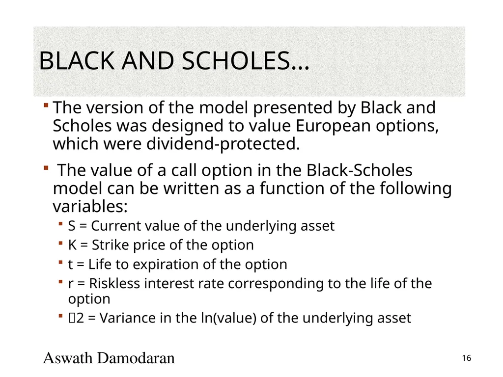
Black and Scholes… The version of the model presented by Black and Scholes was designed to value European options, which were dividend-protected.
The value of a call option in the Black-Scholes model can be written as a function of the following variables:
S = Current value of the underlying asset
K = Strike price of the option
t = Life to expiration of the option
r = Riskless interest rate corresponding to the life of the option
2 = Variance in the ln(value) of the underlying asset Aswath Damodaran 16<br>
The value of a call option in the Black-Scholes model can be written as a function of the following variables:
S = Current value of the underlying asset
K = Strike price of the option
t = Life to expiration of the option
r = Riskless interest rate corresponding to the life of the option
2 = Variance in the ln(value) of the underlying asset Aswath Damodaran 16<br>
17
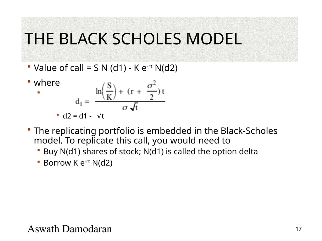
The Black Scholes Model Value of call = S N (d1) - K e-rt N(d2)
where
d2 = d1 - √t
The replicating portfolio is embedded in the Black-Scholes model. To replicate this call, you would need to
Buy N(d1) shares of stock; N(d1) is called the option delta
Borrow K e-rt N(d2) Aswath Damodaran 17<br>
where
d2 = d1 - √t
The replicating portfolio is embedded in the Black-Scholes model. To replicate this call, you would need to
Buy N(d1) shares of stock; N(d1) is called the option delta
Borrow K e-rt N(d2) Aswath Damodaran 17<br>
18
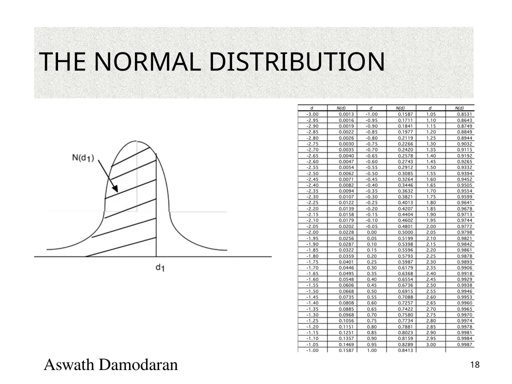
The Normal Distribution Aswath Damodaran 18<br>
19
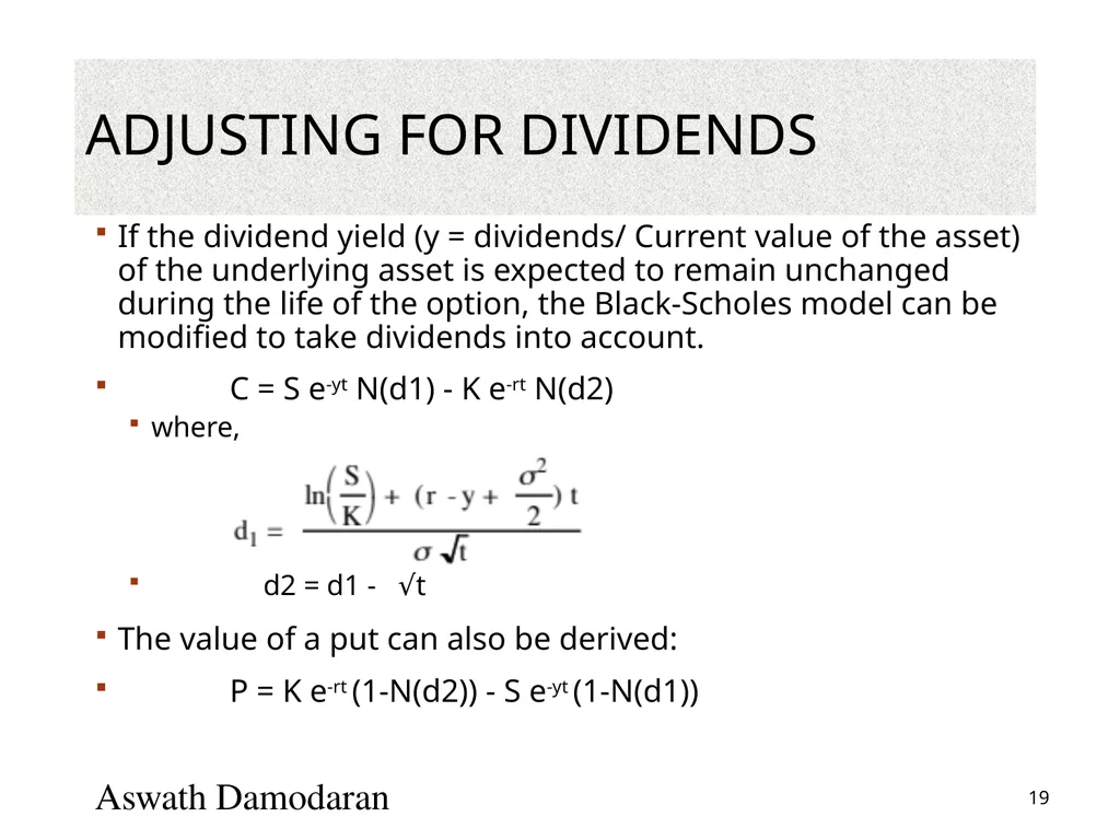
Adjusting for Dividends If the dividend yield (y = dividends/ Current value of the asset) of the underlying asset is expected to remain unchanged during the life of the option, the Black-Scholes model can be modified to take dividends into account.
C = S e-yt N(d1) - K e-rt N(d2)
where,
d2 = d1 - √t
The value of a put can also be derived:
P = K e-rt (1-N(d2)) - S e-yt (1-N(d1)) Aswath Damodaran 19<br>
C = S e-yt N(d1) - K e-rt N(d2)
where,
d2 = d1 - √t
The value of a put can also be derived:
P = K e-rt (1-N(d2)) - S e-yt (1-N(d1)) Aswath Damodaran 19<br>
20
Dividend Yield = Cost of Delay Options have time premiums, and when they are traded, you very seldom get early exercise, with one exception being calls before big ex-dividend dates. The trade off that drives early exercise is:
Loss of the time premium of the option from exercising early (against)
Dividends you will receive, if you exercise early
If the dividend exceeds the time premium, you will see early exercise.
Put differently, the dividends foregone become the cost of delaying exercise and leaving the option live.
Thus, having a cost of delay in an option will require that you use a dividend-adjusted version of the option pricing model. Aswath Damodaran 20<br>
Loss of the time premium of the option from exercising early (against)
Dividends you will receive, if you exercise early
If the dividend exceeds the time premium, you will see early exercise.
Put differently, the dividends foregone become the cost of delaying exercise and leaving the option live.
Thus, having a cost of delay in an option will require that you use a dividend-adjusted version of the option pricing model. Aswath Damodaran 20<br>
21
Choice of Option Pricing Models Most practitioners who use option pricing models to value real options argue for the binomial model over the Black-Scholes and justify this choice by noting that
Early exercise is the rule rather than the exception with real options
Underlying asset values are generally discontinous.
If you can develop a binomial tree with outcomes at each node, it looks a great deal like a decision tree from capital budgeting. The question then becomes when and why the two approaches yield different estimates of value. Aswath Damodaran 21<br>
Early exercise is the rule rather than the exception with real options
Underlying asset values are generally discontinous.
If you can develop a binomial tree with outcomes at each node, it looks a great deal like a decision tree from capital budgeting. The question then becomes when and why the two approaches yield different estimates of value. Aswath Damodaran 21<br>
22
The Decision Tree Alternative Traditional decision tree analysis tends to use
One cost of capital to discount cashflows in each branch to the present
Probabilities to compute an expected value
These values will generally be different from option pricing model values
If you modified decision tree analysis to
Use different discount rates at each node to reflect where you are in the decision tree (This is the Copeland solution) (or)
Use the riskfree rate to discount cashflows in each branch, estimate the probabilities to estimate an expected value and adjust the expected value for the market risk in the investment
Decision Trees could yield the same values as option pricing models Aswath Damodaran 22<br>
One cost of capital to discount cashflows in each branch to the present
Probabilities to compute an expected value
These values will generally be different from option pricing model values
If you modified decision tree analysis to
Use different discount rates at each node to reflect where you are in the decision tree (This is the Copeland solution) (or)
Use the riskfree rate to discount cashflows in each branch, estimate the probabilities to estimate an expected value and adjust the expected value for the market risk in the investment
Decision Trees could yield the same values as option pricing models Aswath Damodaran 22<br>
23
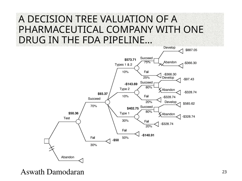
A decision tree valuation of a pharmaceutical company with one drug in the FDA pipeline… Aswath Damodaran 23<br>
24
Key Tests for Real Options Is there an option embedded in this asset/ decision?
Can you identify the underlying asset?
Can you specify the contingency under which you will get payoff?
Is there exclusivity?
If yes, there is option value.
If no, there is none.
If in between, you have to scale value.
Can you use an option pricing model to value the real option?
Is the underlying asset traded?
Can the option be bought and sold?
Is the cost of exercising the option known and clear? Aswath Damodaran 24<br>
Can you identify the underlying asset?
Can you specify the contingency under which you will get payoff?
Is there exclusivity?
If yes, there is option value.
If no, there is none.
If in between, you have to scale value.
Can you use an option pricing model to value the real option?
Is the underlying asset traded?
Can the option be bought and sold?
Is the cost of exercising the option known and clear? Aswath Damodaran 24<br>
25
I. Options in Projects/Investments/Acquisitions One of the limitations of traditional investment analysis is that it is static and does not do a good job of capturing the options embedded in investment.
The first of these options is the option to delay taking a investment, when a firm has exclusive rights to it, until a later date.
The second of these options is taking one investment may allow us to take advantage of other opportunities (investments) in the future
The last option that is embedded in projects is the option to abandon an investment, if the cash flows do not measure up.
These options all add value to projects and may make a “bad” investment (from traditional analysis) into a good one. Aswath Damodaran 25<br>
The first of these options is the option to delay taking a investment, when a firm has exclusive rights to it, until a later date.
The second of these options is taking one investment may allow us to take advantage of other opportunities (investments) in the future
The last option that is embedded in projects is the option to abandon an investment, if the cash flows do not measure up.
These options all add value to projects and may make a “bad” investment (from traditional analysis) into a good one. Aswath Damodaran 25<br>
26
A. The Option to Delay When a firm has exclusive rights to a project or product for a specific period, it can delay taking this project or product until a later date.
A traditional investment analysis just answers the question of whether the project is a “good” one if taken today.
Thus, the fact that a project does not pass muster today (because its NPV is negative, or its IRR is less than its hurdle rate) does not mean that the rights to this project are not valuable. Aswath Damodaran 26<br>
A traditional investment analysis just answers the question of whether the project is a “good” one if taken today.
Thus, the fact that a project does not pass muster today (because its NPV is negative, or its IRR is less than its hurdle rate) does not mean that the rights to this project are not valuable. Aswath Damodaran 26<br>
27
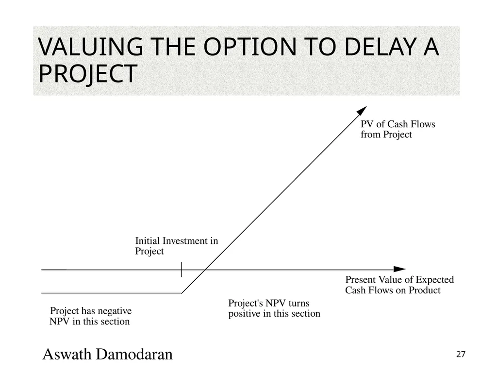
Valuing the Option to Delay a Project Aswath Damodaran 27 Present Value of Expected Cash Flows on Product PV of Cash Flows from Project Initial Investment in Project Project has negative NPV in this section Project's NPV turns positive in this section<br>
28
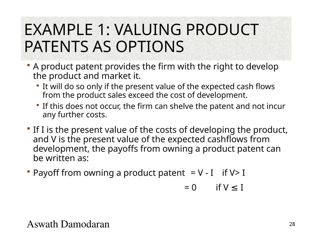
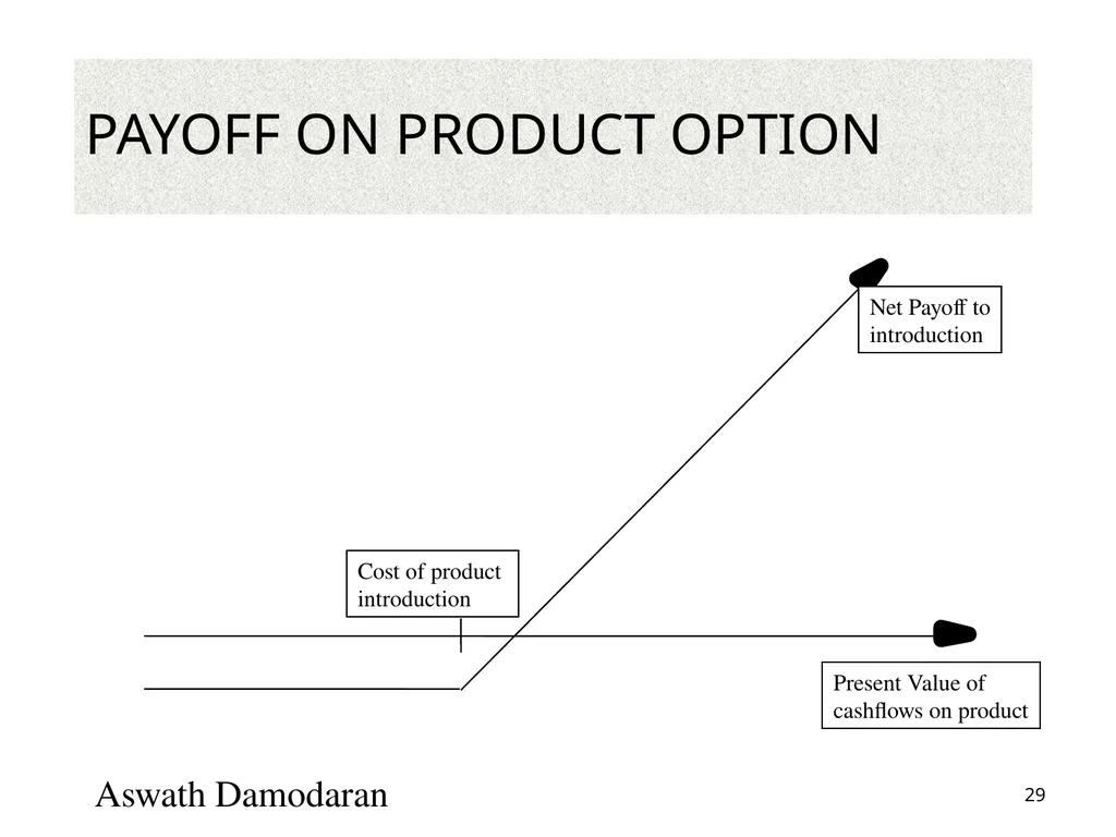
Example 1: Valuing product patents as options A product patent provides the firm with the right to develop the product and market it.
It will do so only if the present value of the expected cash flows from the product sales exceed the cost of development.
If this does not occur, the firm can shelve the patent and not incur any further costs.
If I is the present value of the costs of developing the product, and V is the present value of the expected cashflows from development, the payoffs from owning a product patent can be written as:
Payoff from owning a product patent = V - I if V> I
= 0 if V ≤ I Aswath Damodaran 28<br>
It will do so only if the present value of the expected cash flows from the product sales exceed the cost of development.
If this does not occur, the firm can shelve the patent and not incur any further costs.
If I is the present value of the costs of developing the product, and V is the present value of the expected cashflows from development, the payoffs from owning a product patent can be written as:
Payoff from owning a product patent = V - I if V> I
= 0 if V ≤ I Aswath Damodaran 28<br>
29
Payoff on Product Option Aswath Damodaran 29 Present Value of
cashflows on product Net Payoff to
introduction Cost of product
introduction<br>
cashflows on product Net Payoff to
introduction Cost of product
introduction<br>
30
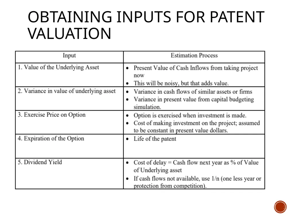
Obtaining Inputs for Patent Valuation<br>
31
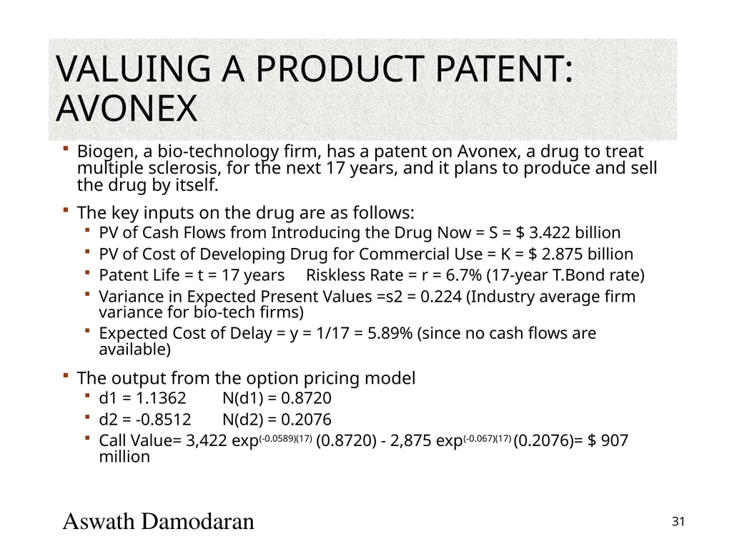
Valuing a Product Patent: Avonex Biogen, a bio-technology firm, has a patent on Avonex, a drug to treat multiple sclerosis, for the next 17 years, and it plans to produce and sell the drug by itself.
The key inputs on the drug are as follows:
PV of Cash Flows from Introducing the Drug Now = S = $ 3.422 billion
PV of Cost of Developing Drug for Commercial Use = K = $ 2.875 billion
Patent Life = t = 17 years Riskless Rate = r = 6.7% (17-year T.Bond rate)
Variance in Expected Present Values =s2 = 0.224 (Industry average firm variance for bio-tech firms)
Expected Cost of Delay = y = 1/17 = 5.89% (since no cash flows are available)
The output from the option pricing model
d1 = 1.1362 N(d1) = 0.8720
d2 = -0.8512 N(d2) = 0.2076
Call Value= 3,422 exp(-0.0589)(17) (0.8720) - 2,875 exp(-0.067)(17) (0.2076)= $ 907 million Aswath Damodaran 31<br>
The key inputs on the drug are as follows:
PV of Cash Flows from Introducing the Drug Now = S = $ 3.422 billion
PV of Cost of Developing Drug for Commercial Use = K = $ 2.875 billion
Patent Life = t = 17 years Riskless Rate = r = 6.7% (17-year T.Bond rate)
Variance in Expected Present Values =s2 = 0.224 (Industry average firm variance for bio-tech firms)
Expected Cost of Delay = y = 1/17 = 5.89% (since no cash flows are available)
The output from the option pricing model
d1 = 1.1362 N(d1) = 0.8720
d2 = -0.8512 N(d2) = 0.2076
Call Value= 3,422 exp(-0.0589)(17) (0.8720) - 2,875 exp(-0.067)(17) (0.2076)= $ 907 million Aswath Damodaran 31<br>
32
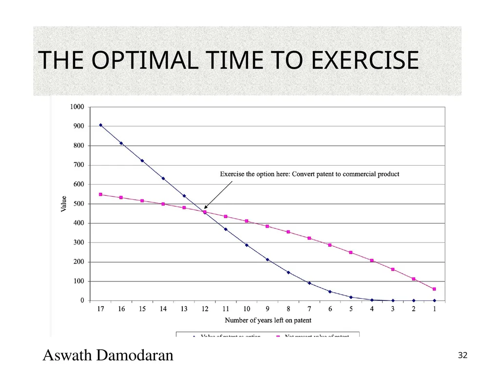
The Optimal Time to Exercise Aswath Damodaran 32<br>
33
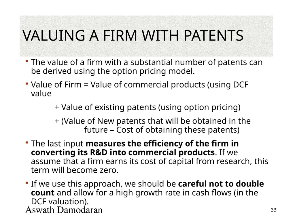
Valuing a firm with patents The value of a firm with a substantial number of patents can be derived using the option pricing model.
Value of Firm = Value of commercial products (using DCF value
+ Value of existing patents (using option pricing)
+ (Value of New patents that will be obtained in the future – Cost of obtaining these patents)
The last input measures the efficiency of the firm in converting its R&D into commercial products. If we assume that a firm earns its cost of capital from research, this term will become zero.
If we use this approach, we should be careful not to double count and allow for a high growth rate in cash flows (in the DCF valuation). Aswath Damodaran 33<br>
Value of Firm = Value of commercial products (using DCF value
+ Value of existing patents (using option pricing)
+ (Value of New patents that will be obtained in the future – Cost of obtaining these patents)
The last input measures the efficiency of the firm in converting its R&D into commercial products. If we assume that a firm earns its cost of capital from research, this term will become zero.
If we use this approach, we should be careful not to double count and allow for a high growth rate in cash flows (in the DCF valuation). Aswath Damodaran 33<br>
34
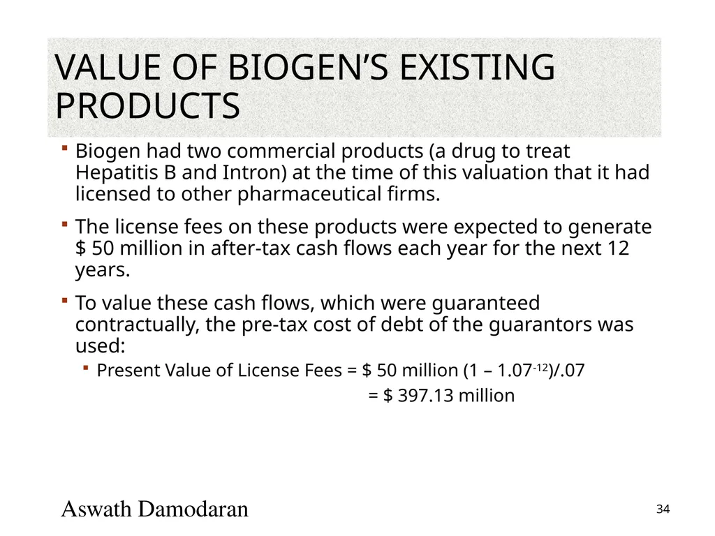
Value of Biogen’s existing products Biogen had two commercial products (a drug to treat Hepatitis B and Intron) at the time of this valuation that it had licensed to other pharmaceutical firms.
The license fees on these products were expected to generate $ 50 million in after-tax cash flows each year for the next 12 years.
To value these cash flows, which were guaranteed contractually, the pre-tax cost of debt of the guarantors was used:
Present Value of License Fees = $ 50 million (1 – 1.07-12)/.07
= $ 397.13 million Aswath Damodaran 34<br>
The license fees on these products were expected to generate $ 50 million in after-tax cash flows each year for the next 12 years.
To value these cash flows, which were guaranteed contractually, the pre-tax cost of debt of the guarantors was used:
Present Value of License Fees = $ 50 million (1 – 1.07-12)/.07
= $ 397.13 million Aswath Damodaran 34<br>
35
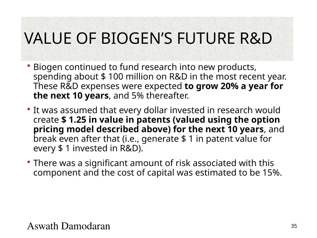
Value of Biogen’s Future R&D Biogen continued to fund research into new products, spending about $ 100 million on R&D in the most recent year. These R&D expenses were expected to grow 20% a year for the next 10 years, and 5% thereafter.
It was assumed that every dollar invested in research would create $ 1.25 in value in patents (valued using the option pricing model described above) for the next 10 years, and break even after that (i.e., generate $ 1 in patent value for every $ 1 invested in R&D).
There was a significant amount of risk associated with this component and the cost of capital was estimated to be 15%. Aswath Damodaran 35<br>
It was assumed that every dollar invested in research would create $ 1.25 in value in patents (valued using the option pricing model described above) for the next 10 years, and break even after that (i.e., generate $ 1 in patent value for every $ 1 invested in R&D).
There was a significant amount of risk associated with this component and the cost of capital was estimated to be 15%. Aswath Damodaran 35<br>
36
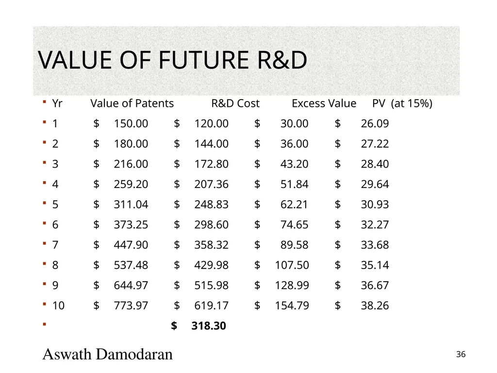
Value of Future R&D Yr Value of Patents R&D Cost Excess Value PV (at 15%)
1 $ 150.00 $ 120.00 $ 30.00 $ 26.09
2 $ 180.00 $ 144.00 $ 36.00 $ 27.22
3 $ 216.00 $ 172.80 $ 43.20 $ 28.40
4 $ 259.20 $ 207.36 $ 51.84 $ 29.64
5 $ 311.04 $ 248.83 $ 62.21 $ 30.93
6 $ 373.25 $ 298.60 $ 74.65 $ 32.27
7 $ 447.90 $ 358.32 $ 89.58 $ 33.68
8 $ 537.48 $ 429.98 $ 107.50 $ 35.14
9 $ 644.97 $ 515.98 $ 128.99 $ 36.67
10 $ 773.97 $ 619.17 $ 154.79 $ 38.26
$ 318.30 Aswath Damodaran 36<br>
1 $ 150.00 $ 120.00 $ 30.00 $ 26.09
2 $ 180.00 $ 144.00 $ 36.00 $ 27.22
3 $ 216.00 $ 172.80 $ 43.20 $ 28.40
4 $ 259.20 $ 207.36 $ 51.84 $ 29.64
5 $ 311.04 $ 248.83 $ 62.21 $ 30.93
6 $ 373.25 $ 298.60 $ 74.65 $ 32.27
7 $ 447.90 $ 358.32 $ 89.58 $ 33.68
8 $ 537.48 $ 429.98 $ 107.50 $ 35.14
9 $ 644.97 $ 515.98 $ 128.99 $ 36.67
10 $ 773.97 $ 619.17 $ 154.79 $ 38.26
$ 318.30 Aswath Damodaran 36<br>
37
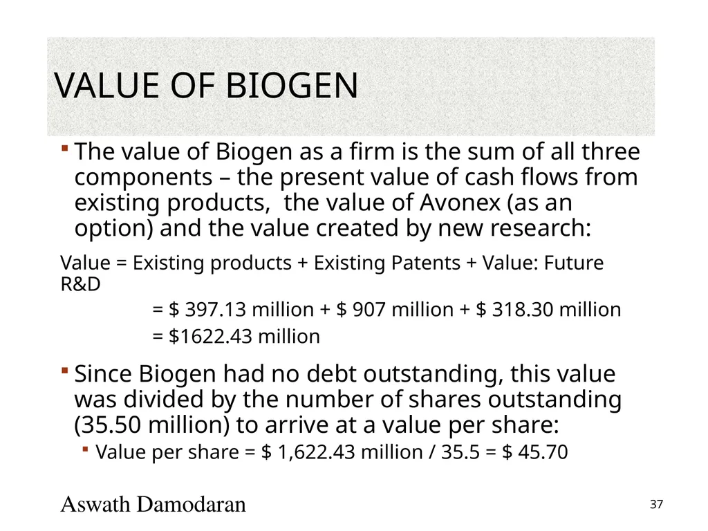
Value of Biogen The value of Biogen as a firm is the sum of all three components – the present value of cash flows from existing products, the value of Avonex (as an option) and the value created by new research:
Value = Existing products + Existing Patents + Value: Future R&D
= $ 397.13 million + $ 907 million + $ 318.30 million
= $1622.43 million
Since Biogen had no debt outstanding, this value was divided by the number of shares outstanding (35.50 million) to arrive at a value per share:
Value per share = $ 1,622.43 million / 35.5 = $ 45.70 Aswath Damodaran 37<br>
Value = Existing products + Existing Patents + Value: Future R&D
= $ 397.13 million + $ 907 million + $ 318.30 million
= $1622.43 million
Since Biogen had no debt outstanding, this value was divided by the number of shares outstanding (35.50 million) to arrive at a value per share:
Value per share = $ 1,622.43 million / 35.5 = $ 45.70 Aswath Damodaran 37<br>
38
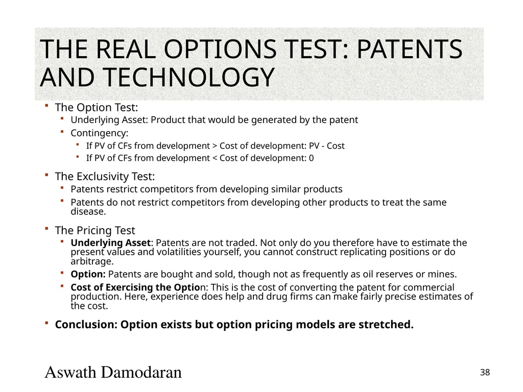
The Real Options Test: Patents and Technology The Option Test:
Underlying Asset: Product that would be generated by the patent
Contingency:
If PV of CFs from development > Cost of development: PV - Cost
If PV of CFs from development < Cost of development: 0
The Exclusivity Test:
Patents restrict competitors from developing similar products
Patents do not restrict competitors from developing other products to treat the same disease.
The Pricing Test
Underlying Asset: Patents are not traded. Not only do you therefore have to estimate the present values and volatilities yourself, you cannot construct replicating positions or do arbitrage.
Option: Patents are bought and sold, though not as frequently as oil reserves or mines.
Cost of Exercising the Option: This is the cost of converting the patent for commercial production. Here, experience does help and drug firms can make fairly precise estimates of the cost.
Conclusion: Option exists but option pricing models are stretched. Aswath Damodaran 38<br>
Underlying Asset: Product that would be generated by the patent
Contingency:
If PV of CFs from development > Cost of development: PV - Cost
If PV of CFs from development < Cost of development: 0
The Exclusivity Test:
Patents restrict competitors from developing similar products
Patents do not restrict competitors from developing other products to treat the same disease.
The Pricing Test
Underlying Asset: Patents are not traded. Not only do you therefore have to estimate the present values and volatilities yourself, you cannot construct replicating positions or do arbitrage.
Option: Patents are bought and sold, though not as frequently as oil reserves or mines.
Cost of Exercising the Option: This is the cost of converting the patent for commercial production. Here, experience does help and drug firms can make fairly precise estimates of the cost.
Conclusion: Option exists but option pricing models are stretched. Aswath Damodaran 38<br>
39
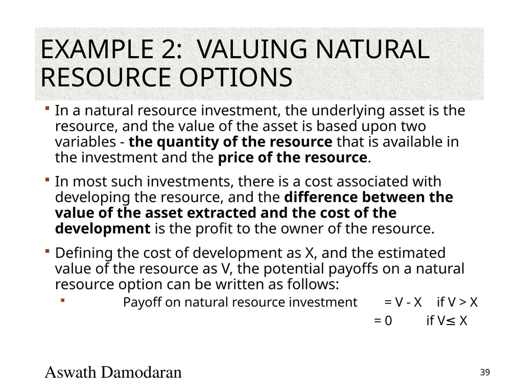
Example 2: Valuing Natural Resource Options In a natural resource investment, the underlying asset is the resource, and the value of the asset is based upon two variables - the quantity of the resource that is available in the investment and the price of the resource.
In most such investments, there is a cost associated with developing the resource, and the difference between the value of the asset extracted and the cost of the development is the profit to the owner of the resource.
Defining the cost of development as X, and the estimated value of the resource as V, the potential payoffs on a natural resource option can be written as follows:
Payoff on natural resource investment = V - X if V > X
= 0 if V≤ X Aswath Damodaran 39<br>
In most such investments, there is a cost associated with developing the resource, and the difference between the value of the asset extracted and the cost of the development is the profit to the owner of the resource.
Defining the cost of development as X, and the estimated value of the resource as V, the potential payoffs on a natural resource option can be written as follows:
Payoff on natural resource investment = V - X if V > X
= 0 if V≤ X Aswath Damodaran 39<br>
40
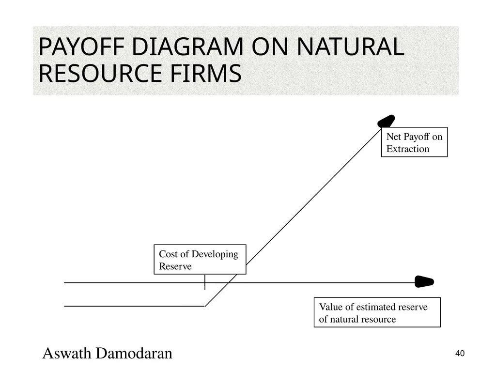
Payoff Diagram on Natural Resource Firms Aswath Damodaran 40 Value of estimated reserve of natural resource Net Payoff on
Extraction Cost of Developing
Reserve<br>
Extraction Cost of Developing
Reserve<br>
41
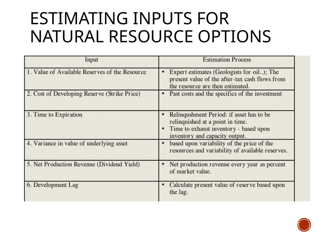
Estimating Inputs for Natural Resource Options<br>
42
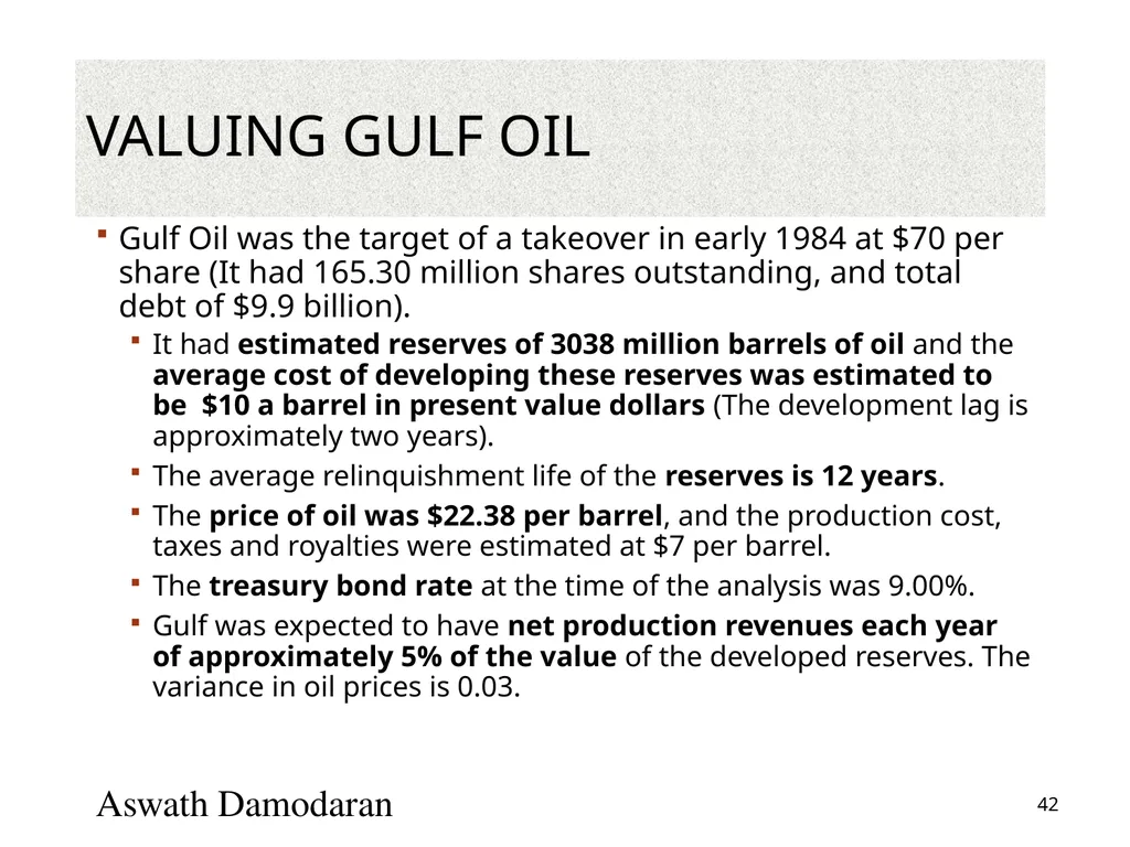
Valuing Gulf Oil Gulf Oil was the target of a takeover in early 1984 at $70 per share (It had 165.30 million shares outstanding, and total debt of $9.9 billion).
It had estimated reserves of 3038 million barrels of oil and the average cost of developing these reserves was estimated to be $10 a barrel in present value dollars (The development lag is approximately two years).
The average relinquishment life of the reserves is 12 years.
The price of oil was $22.38 per barrel, and the production cost, taxes and royalties were estimated at $7 per barrel.
The treasury bond rate at the time of the analysis was 9.00%.
Gulf was expected to have net production revenues each year of approximately 5% of the value of the developed reserves. The variance in oil prices is 0.03. Aswath Damodaran 42<br>
It had estimated reserves of 3038 million barrels of oil and the average cost of developing these reserves was estimated to be $10 a barrel in present value dollars (The development lag is approximately two years).
The average relinquishment life of the reserves is 12 years.
The price of oil was $22.38 per barrel, and the production cost, taxes and royalties were estimated at $7 per barrel.
The treasury bond rate at the time of the analysis was 9.00%.
Gulf was expected to have net production revenues each year of approximately 5% of the value of the developed reserves. The variance in oil prices is 0.03. Aswath Damodaran 42<br>
43
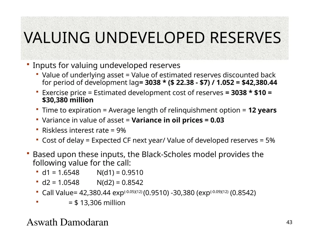
Valuing Undeveloped Reserves Inputs for valuing undeveloped reserves
Value of underlying asset = Value of estimated reserves discounted back for period of development lag= 3038 * ($ 22.38 - $7) / 1.052 = $42,380.44
Exercise price = Estimated development cost of reserves = 3038 * $10 = $30,380 million
Time to expiration = Average length of relinquishment option = 12 years
Variance in value of asset = Variance in oil prices = 0.03
Riskless interest rate = 9%
Cost of delay = Expected CF next year/ Value of developed reserves = 5%
Based upon these inputs, the Black-Scholes model provides the following value for the call:
d1 = 1.6548 N(d1) = 0.9510
d2 = 1.0548 N(d2) = 0.8542
Call Value= 42,380.44 exp(-0.05)(12) (0.9510) -30,380 (exp(-0.09)(12) (0.8542)
= $ 13,306 million Aswath Damodaran 43<br>
Value of underlying asset = Value of estimated reserves discounted back for period of development lag= 3038 * ($ 22.38 - $7) / 1.052 = $42,380.44
Exercise price = Estimated development cost of reserves = 3038 * $10 = $30,380 million
Time to expiration = Average length of relinquishment option = 12 years
Variance in value of asset = Variance in oil prices = 0.03
Riskless interest rate = 9%
Cost of delay = Expected CF next year/ Value of developed reserves = 5%
Based upon these inputs, the Black-Scholes model provides the following value for the call:
d1 = 1.6548 N(d1) = 0.9510
d2 = 1.0548 N(d2) = 0.8542
Call Value= 42,380.44 exp(-0.05)(12) (0.9510) -30,380 (exp(-0.09)(12) (0.8542)
= $ 13,306 million Aswath Damodaran 43<br>
44
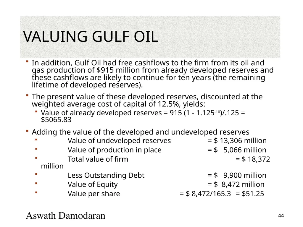
Valuing Gulf Oil In addition, Gulf Oil had free cashflows to the firm from its oil and gas production of $915 million from already developed reserves and these cashflows are likely to continue for ten years (the remaining lifetime of developed reserves).
The present value of these developed reserves, discounted at the weighted average cost of capital of 12.5%, yields:
Value of already developed reserves = 915 (1 - 1.125-10)/.125 = $5065.83
Adding the value of the developed and undeveloped reserves
Value of undeveloped reserves = $ 13,306 million
Value of production in place = $ 5,066 million
Total value of firm = $ 18,372 million
Less Outstanding Debt = $ 9,900 million
Value of Equity = $ 8,472 million
Value per share = $ 8,472/165.3 = $51.25 Aswath Damodaran 44<br>
The present value of these developed reserves, discounted at the weighted average cost of capital of 12.5%, yields:
Value of already developed reserves = 915 (1 - 1.125-10)/.125 = $5065.83
Adding the value of the developed and undeveloped reserves
Value of undeveloped reserves = $ 13,306 million
Value of production in place = $ 5,066 million
Total value of firm = $ 18,372 million
Less Outstanding Debt = $ 9,900 million
Value of Equity = $ 8,472 million
Value per share = $ 8,472/165.3 = $51.25 Aswath Damodaran 44<br>
45
B. The Option to Expand/Take Other Projects Taking a project today may allow access to other valuable projects in the future.
Thus, even though a project may have a negative NPV, it may be a project worth taking if the option it provides the firm (to take other projects in the future) provides a more-than-compensating value.
These are the options that firms often call “strategic options” and use as a rationale for taking on “negative NPV” or even “negative return” projects. Aswath Damodaran 45<br>
Thus, even though a project may have a negative NPV, it may be a project worth taking if the option it provides the firm (to take other projects in the future) provides a more-than-compensating value.
These are the options that firms often call “strategic options” and use as a rationale for taking on “negative NPV” or even “negative return” projects. Aswath Damodaran 45<br>
46
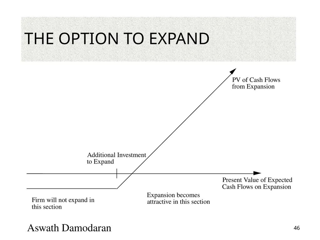
The Option to Expand Aswath Damodaran 46 Present Value of Expected Cash Flows on Expansion PV of Cash Flows from Expansion Additional Investment to Expand Firm will not expand in this section Expansion becomes attractive in this section<br>
47
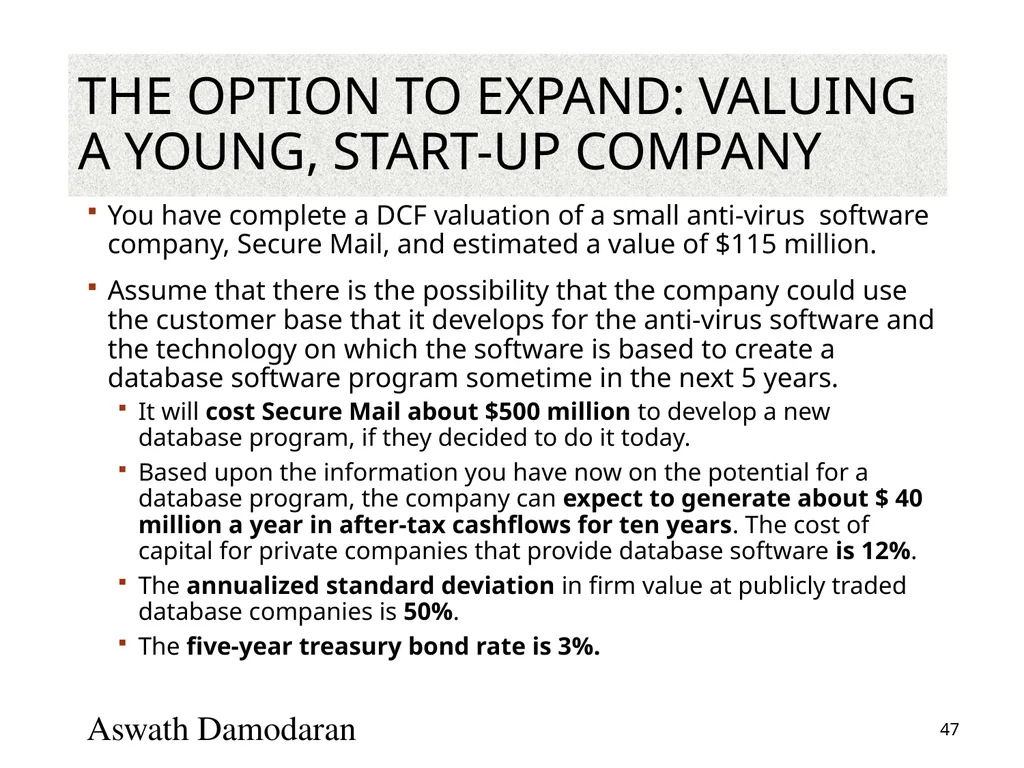
The option to expand: Valuing a young, start-up company You have complete a DCF valuation of a small anti-virus software company, Secure Mail, and estimated a value of $115 million.
Assume that there is the possibility that the company could use the customer base that it develops for the anti-virus software and the technology on which the software is based to create a database software program sometime in the next 5 years.
It will cost Secure Mail about $500 million to develop a new database program, if they decided to do it today.
Based upon the information you have now on the potential for a database program, the company can expect to generate about $ 40 million a year in after-tax cashflows for ten years. The cost of capital for private companies that provide database software is 12%.
The annualized standard deviation in firm value at publicly traded database companies is 50%.
The five-year treasury bond rate is 3%. Aswath Damodaran 47<br>
Assume that there is the possibility that the company could use the customer base that it develops for the anti-virus software and the technology on which the software is based to create a database software program sometime in the next 5 years.
It will cost Secure Mail about $500 million to develop a new database program, if they decided to do it today.
Based upon the information you have now on the potential for a database program, the company can expect to generate about $ 40 million a year in after-tax cashflows for ten years. The cost of capital for private companies that provide database software is 12%.
The annualized standard deviation in firm value at publicly traded database companies is 50%.
The five-year treasury bond rate is 3%. Aswath Damodaran 47<br>
48
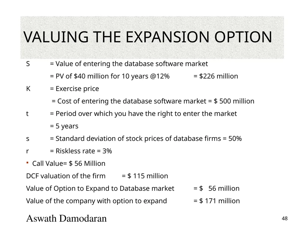
Valuing the Expansion Option S = Value of entering the database software market
= PV of $40 million for 10 years @12% = $226 million
K = Exercise price
= Cost of entering the database software market = $ 500 million
t = Period over which you have the right to enter the market
= 5 years
s = Standard deviation of stock prices of database firms = 50%
r = Riskless rate = 3%
Call Value= $ 56 Million
DCF valuation of the firm = $ 115 million
Value of Option to Expand to Database market = $ 56 million
Value of the company with option to expand = $ 171 million Aswath Damodaran 48<br>
= PV of $40 million for 10 years @12% = $226 million
K = Exercise price
= Cost of entering the database software market = $ 500 million
t = Period over which you have the right to enter the market
= 5 years
s = Standard deviation of stock prices of database firms = 50%
r = Riskless rate = 3%
Call Value= $ 56 Million
DCF valuation of the firm = $ 115 million
Value of Option to Expand to Database market = $ 56 million
Value of the company with option to expand = $ 171 million Aswath Damodaran 48<br>
49
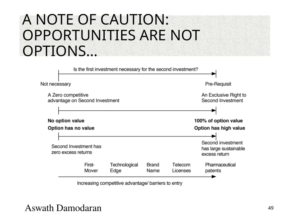
A note of caution: Opportunities are not options… Aswath Damodaran 49<br>
50
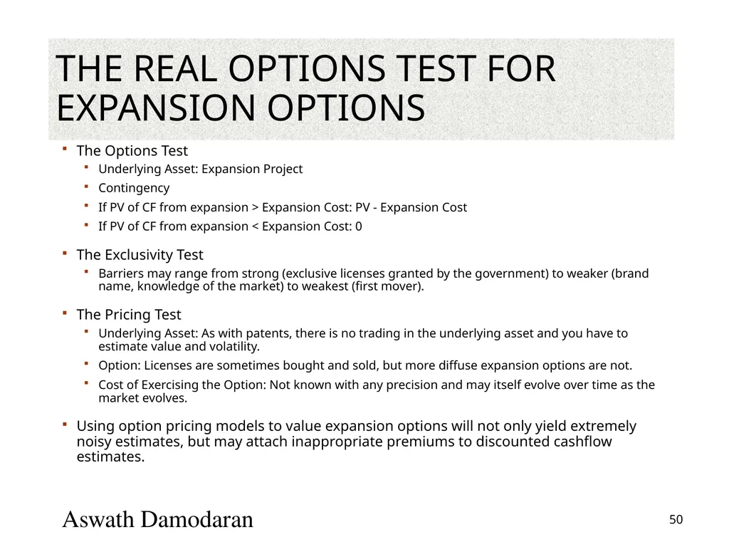
The Real Options Test for Expansion Options The Options Test
Underlying Asset: Expansion Project
Contingency
If PV of CF from expansion > Expansion Cost: PV - Expansion Cost
If PV of CF from expansion < Expansion Cost: 0
The Exclusivity Test
Barriers may range from strong (exclusive licenses granted by the government) to weaker (brand name, knowledge of the market) to weakest (first mover).
The Pricing Test
Underlying Asset: As with patents, there is no trading in the underlying asset and you have to estimate value and volatility.
Option: Licenses are sometimes bought and sold, but more diffuse expansion options are not.
Cost of Exercising the Option: Not known with any precision and may itself evolve over time as the market evolves.
Using option pricing models to value expansion options will not only yield extremely noisy estimates, but may attach inappropriate premiums to discounted cashflow estimates. Aswath Damodaran 50<br>
Underlying Asset: Expansion Project
Contingency
If PV of CF from expansion > Expansion Cost: PV - Expansion Cost
If PV of CF from expansion < Expansion Cost: 0
The Exclusivity Test
Barriers may range from strong (exclusive licenses granted by the government) to weaker (brand name, knowledge of the market) to weakest (first mover).
The Pricing Test
Underlying Asset: As with patents, there is no trading in the underlying asset and you have to estimate value and volatility.
Option: Licenses are sometimes bought and sold, but more diffuse expansion options are not.
Cost of Exercising the Option: Not known with any precision and may itself evolve over time as the market evolves.
Using option pricing models to value expansion options will not only yield extremely noisy estimates, but may attach inappropriate premiums to discounted cashflow estimates. Aswath Damodaran 50<br>
51
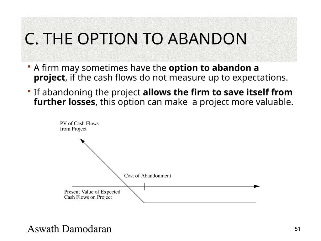
C. The Option to Abandon A firm may sometimes have the option to abandon a project, if the cash flows do not measure up to expectations.
If abandoning the project allows the firm to save itself from further losses, this option can make a project more valuable. Aswath Damodaran 51 Present Value of Expected Cash Flows on Project PV of Cash Flows from Project Cost of Abandonment<br>
If abandoning the project allows the firm to save itself from further losses, this option can make a project more valuable. Aswath Damodaran 51 Present Value of Expected Cash Flows on Project PV of Cash Flows from Project Cost of Abandonment<br>
52
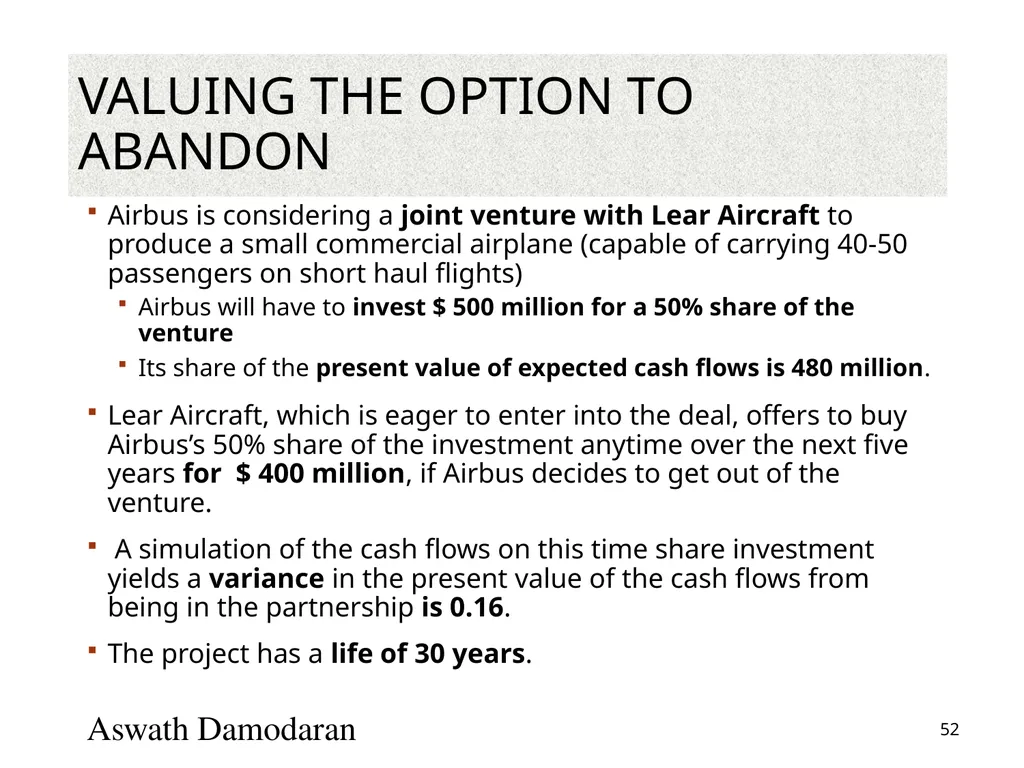
Valuing the Option to Abandon Airbus is considering a joint venture with Lear Aircraft to produce a small commercial airplane (capable of carrying 40-50 passengers on short haul flights)
Airbus will have to invest $ 500 million for a 50% share of the venture
Its share of the present value of expected cash flows is 480 million.
Lear Aircraft, which is eager to enter into the deal, offers to buy Airbus’s 50% share of the investment anytime over the next five years for $ 400 million, if Airbus decides to get out of the venture.
A simulation of the cash flows on this time share investment yields a variance in the present value of the cash flows from being in the partnership is 0.16.
The project has a life of 30 years. Aswath Damodaran 52<br>
Airbus will have to invest $ 500 million for a 50% share of the venture
Its share of the present value of expected cash flows is 480 million.
Lear Aircraft, which is eager to enter into the deal, offers to buy Airbus’s 50% share of the investment anytime over the next five years for $ 400 million, if Airbus decides to get out of the venture.
A simulation of the cash flows on this time share investment yields a variance in the present value of the cash flows from being in the partnership is 0.16.
The project has a life of 30 years. Aswath Damodaran 52<br>
53
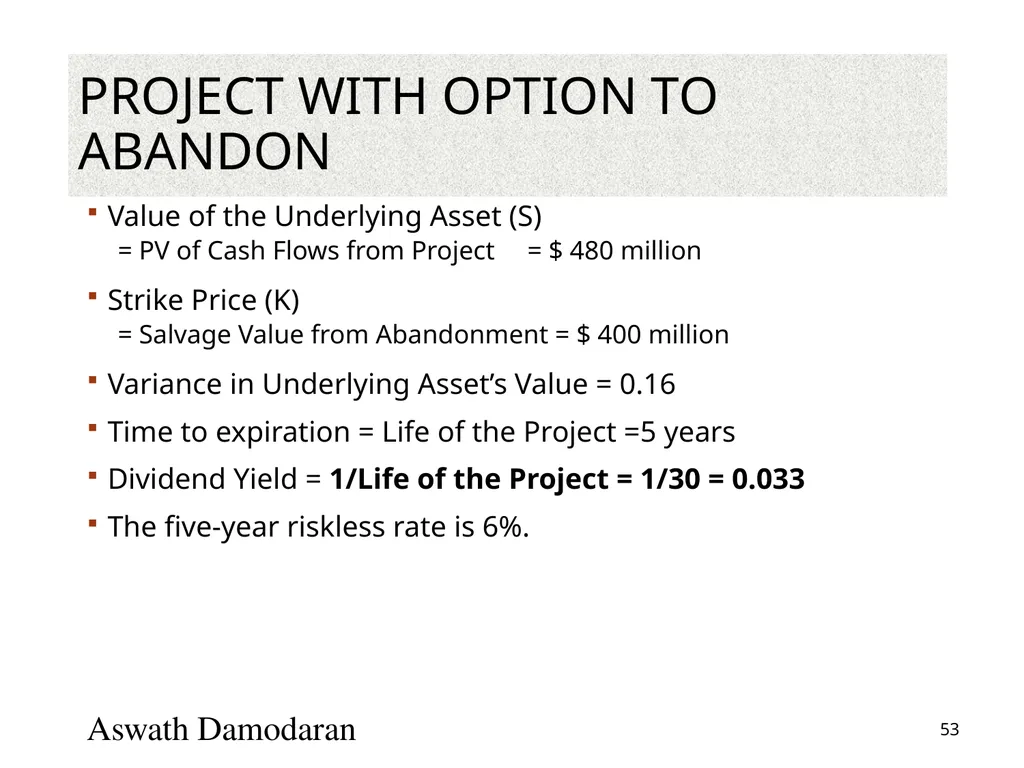
Project with Option to Abandon Value of the Underlying Asset (S)
= PV of Cash Flows from Project = $ 480 million
Strike Price (K)
= Salvage Value from Abandonment = $ 400 million
Variance in Underlying Asset’s Value = 0.16
Time to expiration = Life of the Project =5 years
Dividend Yield = 1/Life of the Project = 1/30 = 0.033
The five-year riskless rate is 6%. Aswath Damodaran 53<br>
= PV of Cash Flows from Project = $ 480 million
Strike Price (K)
= Salvage Value from Abandonment = $ 400 million
Variance in Underlying Asset’s Value = 0.16
Time to expiration = Life of the Project =5 years
Dividend Yield = 1/Life of the Project = 1/30 = 0.033
The five-year riskless rate is 6%. Aswath Damodaran 53<br>
54
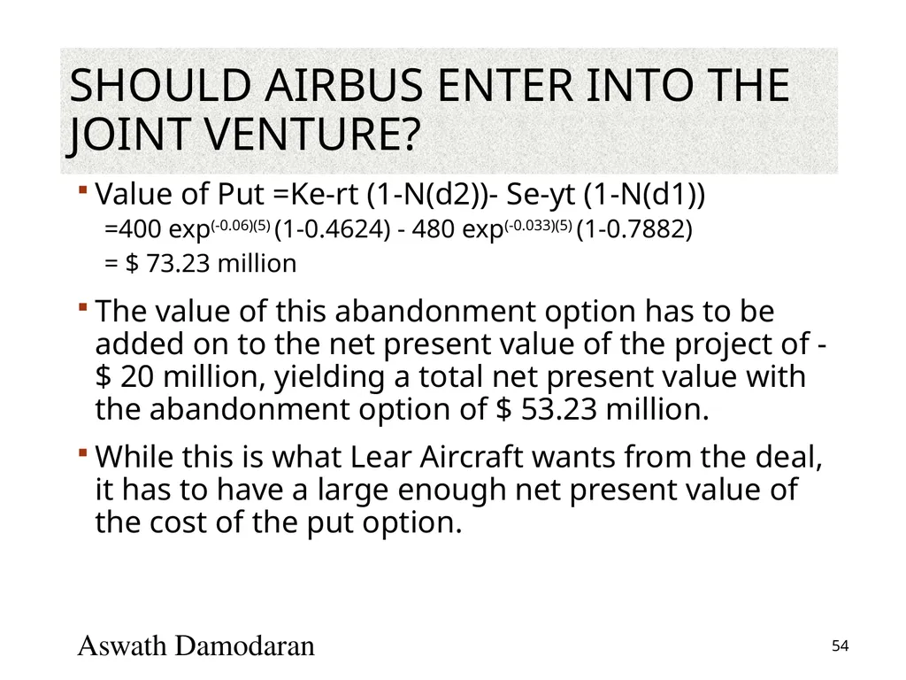
Should Airbus enter into the joint venture? Value of Put =Ke-rt (1-N(d2))- Se-yt (1-N(d1))
=400 exp(-0.06)(5) (1-0.4624) - 480 exp(-0.033)(5) (1-0.7882)
= $ 73.23 million
The value of this abandonment option has to be added on to the net present value of the project of -$ 20 million, yielding a total net present value with the abandonment option of $ 53.23 million.
While this is what Lear Aircraft wants from the deal, it has to have a large enough net present value of the cost of the put option. Aswath Damodaran 54<br>
=400 exp(-0.06)(5) (1-0.4624) - 480 exp(-0.033)(5) (1-0.7882)
= $ 73.23 million
The value of this abandonment option has to be added on to the net present value of the project of -$ 20 million, yielding a total net present value with the abandonment option of $ 53.23 million.
While this is what Lear Aircraft wants from the deal, it has to have a large enough net present value of the cost of the put option. Aswath Damodaran 54<br>
55
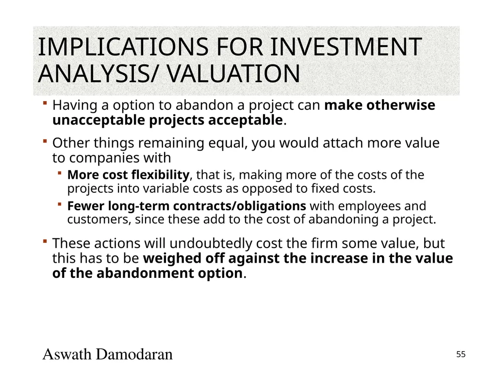
Implications for Investment Analysis/ Valuation Having a option to abandon a project can make otherwise unacceptable projects acceptable.
Other things remaining equal, you would attach more value to companies with
More cost flexibility, that is, making more of the costs of the projects into variable costs as opposed to fixed costs.
Fewer long-term contracts/obligations with employees and customers, since these add to the cost of abandoning a project.
These actions will undoubtedly cost the firm some value, but this has to be weighed off against the increase in the value of the abandonment option. Aswath Damodaran 55<br>
Other things remaining equal, you would attach more value to companies with
More cost flexibility, that is, making more of the costs of the projects into variable costs as opposed to fixed costs.
Fewer long-term contracts/obligations with employees and customers, since these add to the cost of abandoning a project.
These actions will undoubtedly cost the firm some value, but this has to be weighed off against the increase in the value of the abandonment option. Aswath Damodaran 55<br>
56
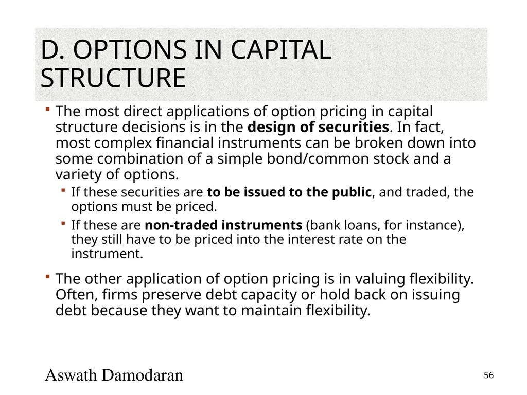
D. Options in Capital Structure The most direct applications of option pricing in capital structure decisions is in the design of securities. In fact, most complex financial instruments can be broken down into some combination of a simple bond/common stock and a variety of options.
If these securities are to be issued to the public, and traded, the options must be priced.
If these are non-traded instruments (bank loans, for instance), they still have to be priced into the interest rate on the instrument.
The other application of option pricing is in valuing flexibility. Often, firms preserve debt capacity or hold back on issuing debt because they want to maintain flexibility. Aswath Damodaran 56<br>
If these securities are to be issued to the public, and traded, the options must be priced.
If these are non-traded instruments (bank loans, for instance), they still have to be priced into the interest rate on the instrument.
The other application of option pricing is in valuing flexibility. Often, firms preserve debt capacity or hold back on issuing debt because they want to maintain flexibility. Aswath Damodaran 56<br>
57
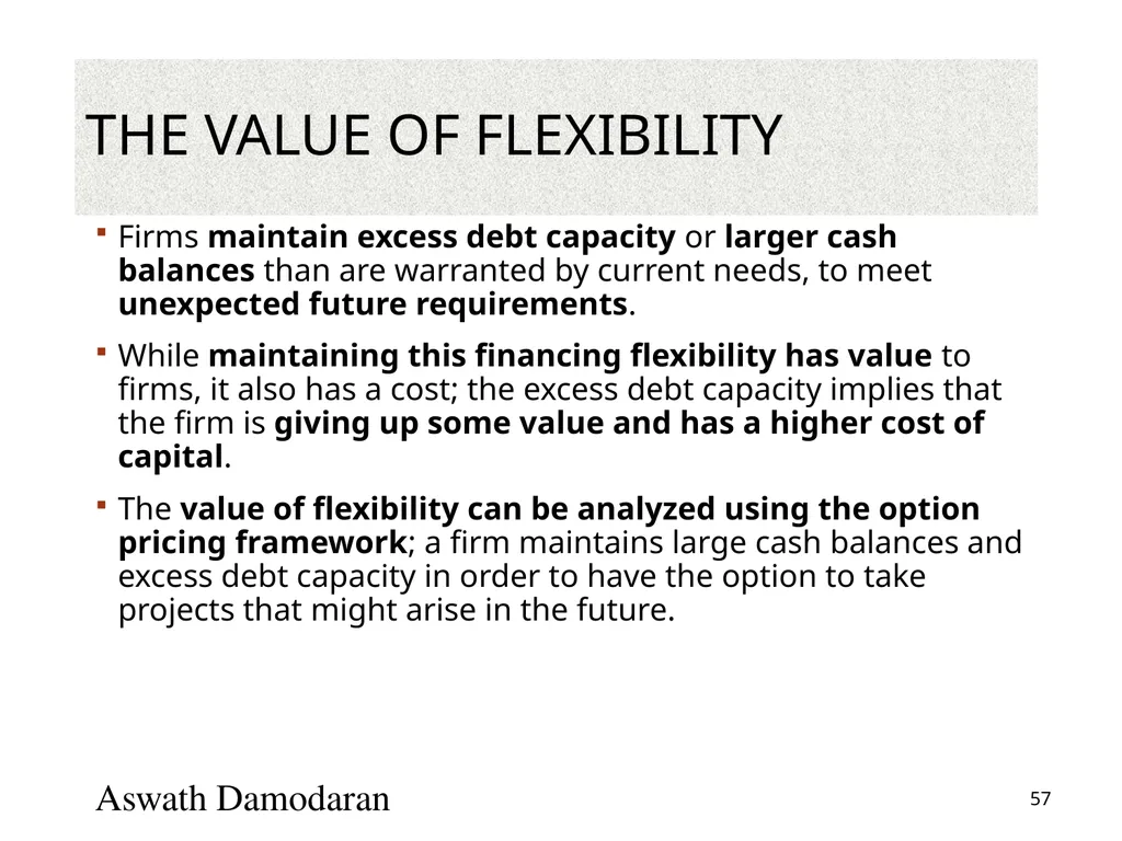
The Value of Flexibility Firms maintain excess debt capacity or larger cash balances than are warranted by current needs, to meet unexpected future requirements.
While maintaining this financing flexibility has value to firms, it also has a cost; the excess debt capacity implies that the firm is giving up some value and has a higher cost of capital.
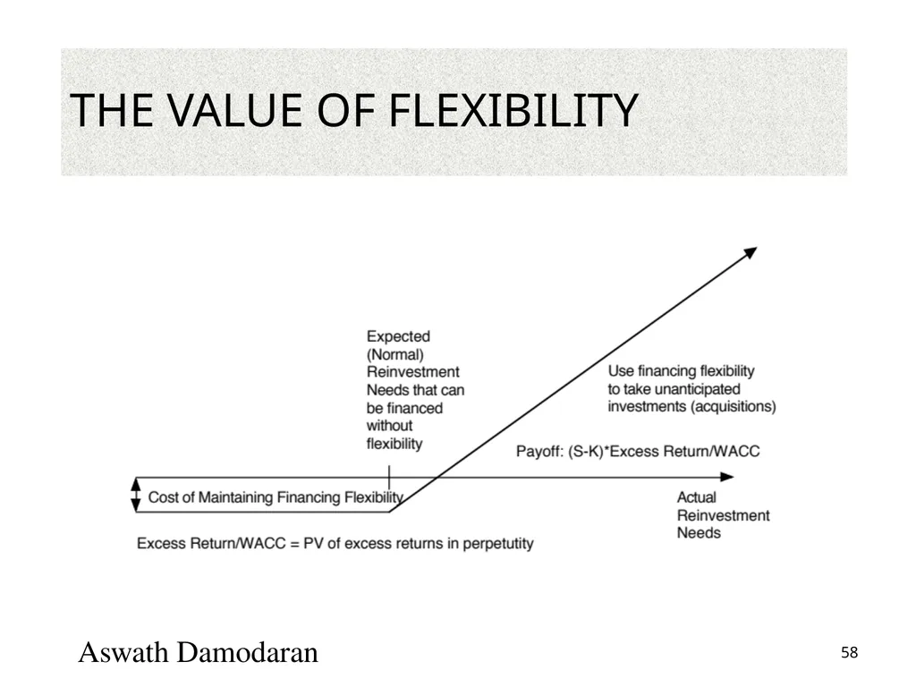
The value of flexibility can be analyzed using the option pricing framework; a firm maintains large cash balances and excess debt capacity in order to have the option to take projects that might arise in the future. Aswath Damodaran 57<br>
While maintaining this financing flexibility has value to firms, it also has a cost; the excess debt capacity implies that the firm is giving up some value and has a higher cost of capital.
The value of flexibility can be analyzed using the option pricing framework; a firm maintains large cash balances and excess debt capacity in order to have the option to take projects that might arise in the future. Aswath Damodaran 57<br>
58
The Value of Flexibility Aswath Damodaran 58<br>
59
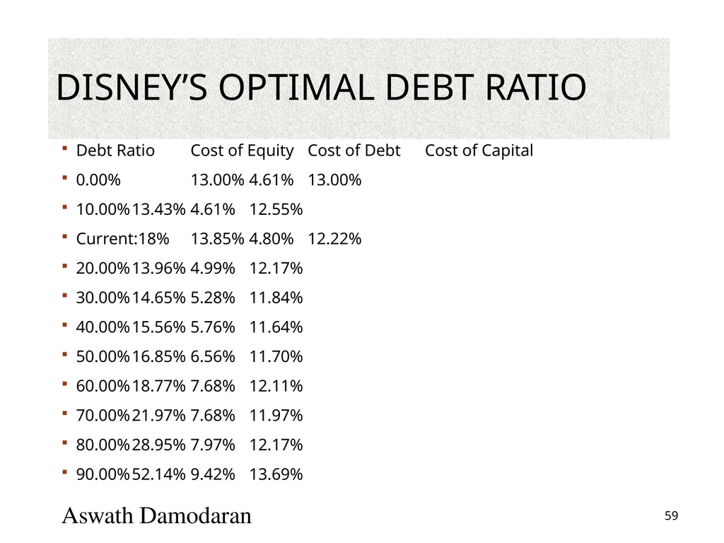
Disney’s Optimal Debt Ratio Debt Ratio Cost of Equity Cost of Debt Cost of Capital
0.00% 13.00% 4.61% 13.00%
10.00% 13.43% 4.61% 12.55%
Current:18% 13.85% 4.80% 12.22%
20.00% 13.96% 4.99% 12.17%
30.00% 14.65% 5.28% 11.84%
40.00% 15.56% 5.76% 11.64%
50.00% 16.85% 6.56% 11.70%
60.00% 18.77% 7.68% 12.11%
70.00% 21.97% 7.68% 11.97%
80.00% 28.95% 7.97% 12.17%
90.00% 52.14% 9.42% 13.69% Aswath Damodaran 59<br>
0.00% 13.00% 4.61% 13.00%
10.00% 13.43% 4.61% 12.55%
Current:18% 13.85% 4.80% 12.22%
20.00% 13.96% 4.99% 12.17%
30.00% 14.65% 5.28% 11.84%
40.00% 15.56% 5.76% 11.64%
50.00% 16.85% 6.56% 11.70%
60.00% 18.77% 7.68% 12.11%
70.00% 21.97% 7.68% 11.97%
80.00% 28.95% 7.97% 12.17%
90.00% 52.14% 9.42% 13.69% Aswath Damodaran 59<br>
60
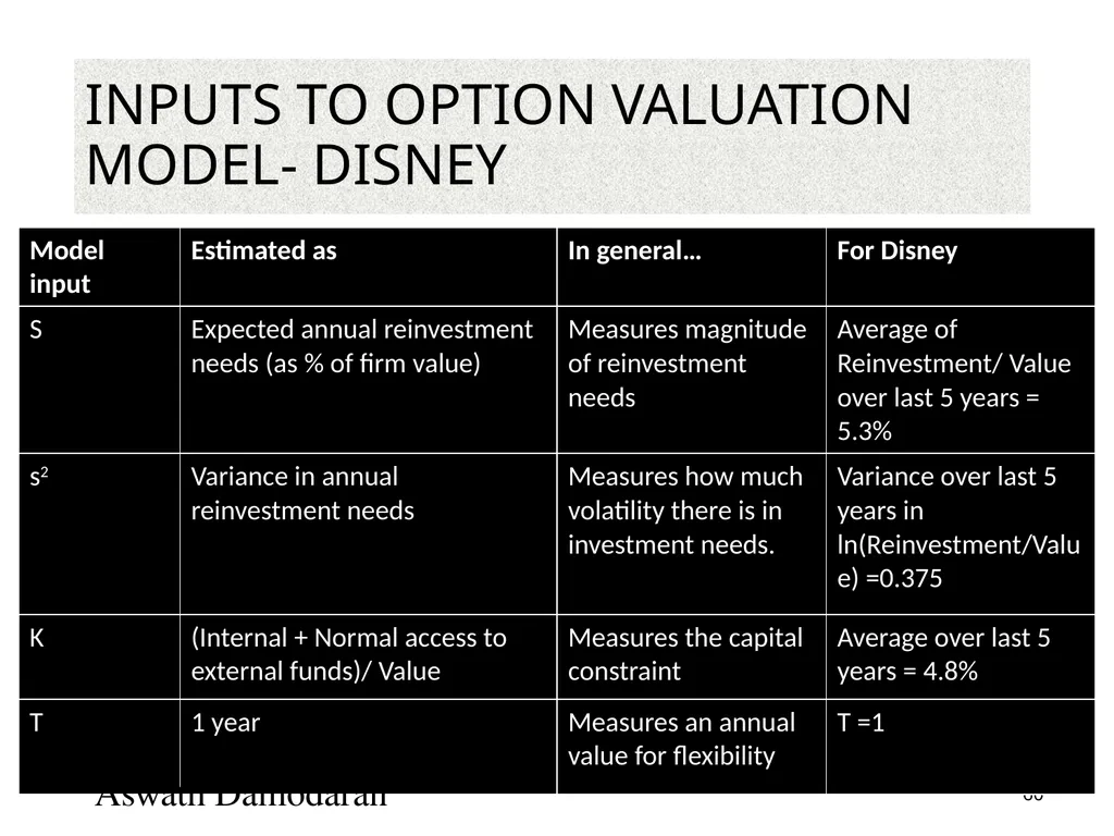
Inputs to Option Valuation Model- Disney Aswath Damodaran 60<br>
61
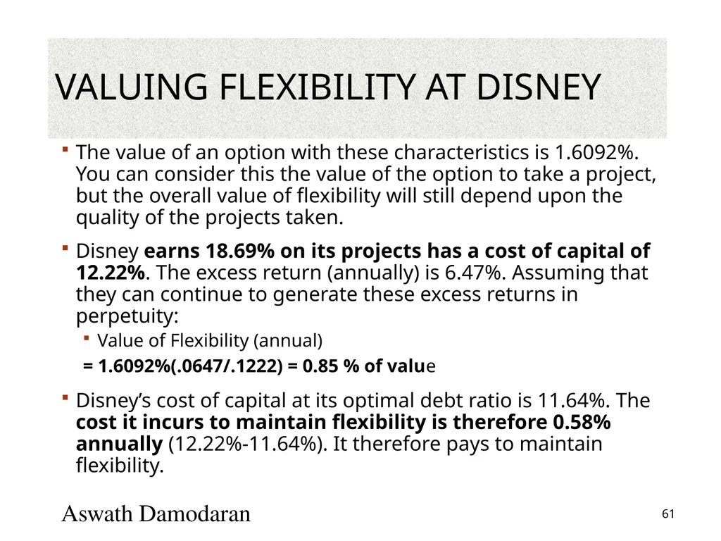
Valuing Flexibility at Disney The value of an option with these characteristics is 1.6092%. You can consider this the value of the option to take a project, but the overall value of flexibility will still depend upon the quality of the projects taken.
Disney earns 18.69% on its projects has a cost of capital of 12.22%. The excess return (annually) is 6.47%. Assuming that they can continue to generate these excess returns in perpetuity:
Value of Flexibility (annual)
= 1.6092%(.0647/.1222) = 0.85 % of value
Disney’s cost of capital at its optimal debt ratio is 11.64%. The cost it incurs to maintain flexibility is therefore 0.58% annually (12.22%-11.64%). It therefore pays to maintain flexibility. Aswath Damodaran 61<br>
Disney earns 18.69% on its projects has a cost of capital of 12.22%. The excess return (annually) is 6.47%. Assuming that they can continue to generate these excess returns in perpetuity:
Value of Flexibility (annual)
= 1.6092%(.0647/.1222) = 0.85 % of value
Disney’s cost of capital at its optimal debt ratio is 11.64%. The cost it incurs to maintain flexibility is therefore 0.58% annually (12.22%-11.64%). It therefore pays to maintain flexibility. Aswath Damodaran 61<br>
62
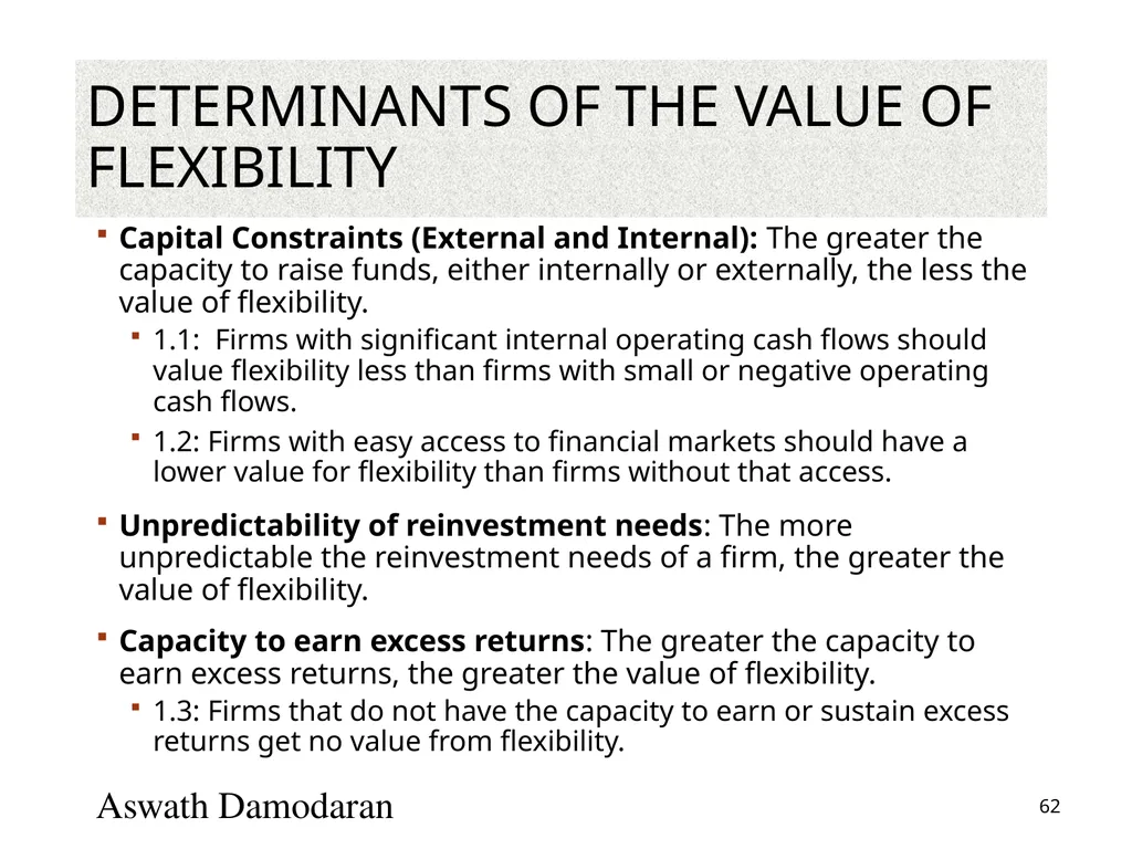
Determinants of the Value of Flexibility Capital Constraints (External and Internal): The greater the capacity to raise funds, either internally or externally, the less the value of flexibility.
1.1: Firms with significant internal operating cash flows should value flexibility less than firms with small or negative operating cash flows.
1.2: Firms with easy access to financial markets should have a lower value for flexibility than firms without that access.
Unpredictability of reinvestment needs: The more unpredictable the reinvestment needs of a firm, the greater the value of flexibility.
Capacity to earn excess returns: The greater the capacity to earn excess returns, the greater the value of flexibility.
1.3: Firms that do not have the capacity to earn or sustain excess returns get no value from flexibility. Aswath Damodaran 62<br>
1.1: Firms with significant internal operating cash flows should value flexibility less than firms with small or negative operating cash flows.
1.2: Firms with easy access to financial markets should have a lower value for flexibility than firms without that access.
Unpredictability of reinvestment needs: The more unpredictable the reinvestment needs of a firm, the greater the value of flexibility.
Capacity to earn excess returns: The greater the capacity to earn excess returns, the greater the value of flexibility.
1.3: Firms that do not have the capacity to earn or sustain excess returns get no value from flexibility. Aswath Damodaran 62<br>
63
E. Valuing Equity as an option The equity in a firm is a residual claim, i.e., equity holders lay claim to all cashflows left over after other financial claim-holders (debt, preferred stock etc.) have been satisfied.
If a firm is liquidated, the same principle applies, with equity investors receiving whatever is left over in the firm after all outstanding debts and other financial claims are paid off.
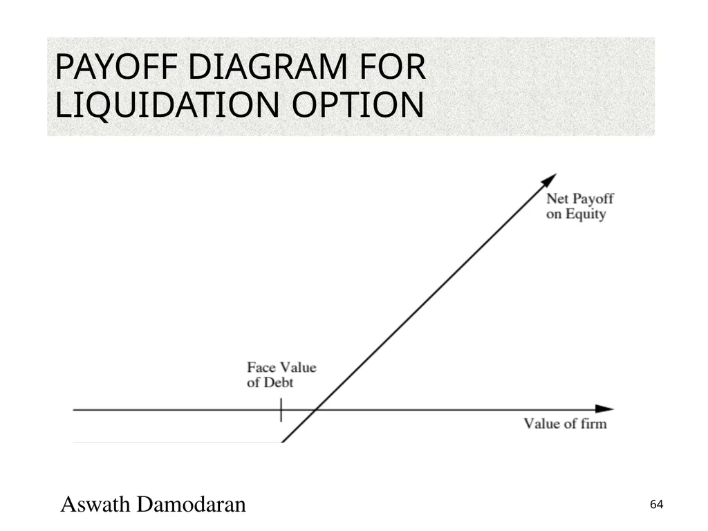
The principle of limited liability, however, protects equity investors in publicly traded firms if the value of the firm is less than the value of the outstanding debt, and they cannot lose more than their investment in the firm. Aswath Damodaran 63<br>
If a firm is liquidated, the same principle applies, with equity investors receiving whatever is left over in the firm after all outstanding debts and other financial claims are paid off.
The principle of limited liability, however, protects equity investors in publicly traded firms if the value of the firm is less than the value of the outstanding debt, and they cannot lose more than their investment in the firm. Aswath Damodaran 63<br>
64
Payoff Diagram for Liquidation Option Aswath Damodaran 64<br>
65
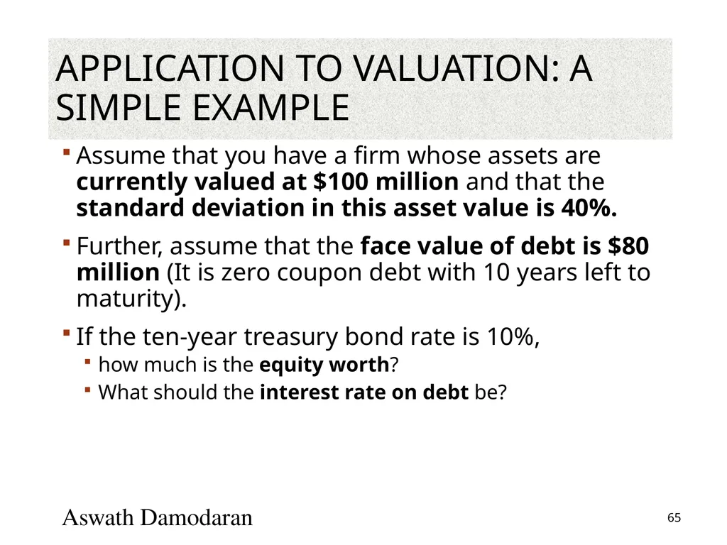
Application to valuation: A simple example Assume that you have a firm whose assets are currently valued at $100 million and that the standard deviation in this asset value is 40%.
Further, assume that the face value of debt is $80 million (It is zero coupon debt with 10 years left to maturity).
If the ten-year treasury bond rate is 10%,
how much is the equity worth?
What should the interest rate on debt be? Aswath Damodaran 65<br>
Further, assume that the face value of debt is $80 million (It is zero coupon debt with 10 years left to maturity).
If the ten-year treasury bond rate is 10%,
how much is the equity worth?
What should the interest rate on debt be? Aswath Damodaran 65<br>
66
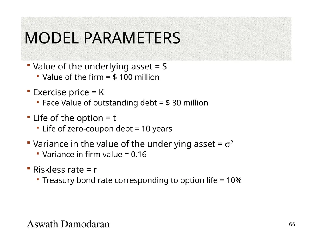
Model Parameters Value of the underlying asset = S
Value of the firm = $ 100 million
Exercise price = K
Face Value of outstanding debt = $ 80 million
Life of the option = t
Life of zero-coupon debt = 10 years
Variance in the value of the underlying asset = s2
Variance in firm value = 0.16
Riskless rate = r
Treasury bond rate corresponding to option life = 10% Aswath Damodaran 66<br>
Value of the firm = $ 100 million
Exercise price = K
Face Value of outstanding debt = $ 80 million
Life of the option = t
Life of zero-coupon debt = 10 years
Variance in the value of the underlying asset = s2
Variance in firm value = 0.16
Riskless rate = r
Treasury bond rate corresponding to option life = 10% Aswath Damodaran 66<br>
67
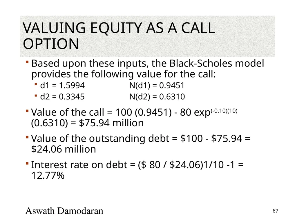
Valuing Equity as a Call Option Based upon these inputs, the Black-Scholes model provides the following value for the call:
d1 = 1.5994 N(d1) = 0.9451
d2 = 0.3345 N(d2) = 0.6310
Value of the call = 100 (0.9451) - 80 exp(-0.10)(10) (0.6310) = $75.94 million
Value of the outstanding debt = $100 - $75.94 = $24.06 million
Interest rate on debt = ($ 80 / $24.06)1/10 -1 = 12.77% Aswath Damodaran 67<br>
d1 = 1.5994 N(d1) = 0.9451
d2 = 0.3345 N(d2) = 0.6310
Value of the call = 100 (0.9451) - 80 exp(-0.10)(10) (0.6310) = $75.94 million
Value of the outstanding debt = $100 - $75.94 = $24.06 million
Interest rate on debt = ($ 80 / $24.06)1/10 -1 = 12.77% Aswath Damodaran 67<br>
68
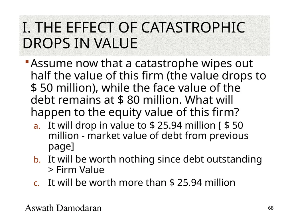
I. The Effect of Catastrophic Drops in Value Assume now that a catastrophe wipes out half the value of this firm (the value drops to $ 50 million), while the face value of the debt remains at $ 80 million. What will happen to the equity value of this firm?
It will drop in value to $ 25.94 million [ $ 50 million - market value of debt from previous page]
It will be worth nothing since debt outstanding > Firm Value
It will be worth more than $ 25.94 million Aswath Damodaran 68<br>
It will drop in value to $ 25.94 million [ $ 50 million - market value of debt from previous page]
It will be worth nothing since debt outstanding > Firm Value
It will be worth more than $ 25.94 million Aswath Damodaran 68<br>
69
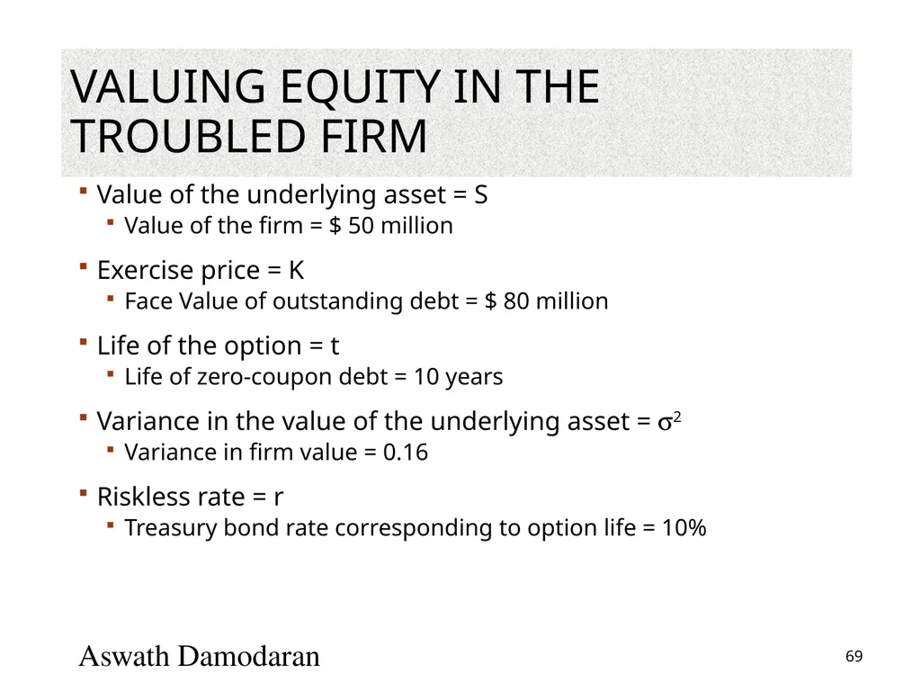
Valuing Equity in the Troubled Firm Value of the underlying asset = S
Value of the firm = $ 50 million
Exercise price = K
Face Value of outstanding debt = $ 80 million
Life of the option = t
Life of zero-coupon debt = 10 years
Variance in the value of the underlying asset = s2
Variance in firm value = 0.16
Riskless rate = r
Treasury bond rate corresponding to option life = 10% Aswath Damodaran 69<br>
Value of the firm = $ 50 million
Exercise price = K
Face Value of outstanding debt = $ 80 million
Life of the option = t
Life of zero-coupon debt = 10 years
Variance in the value of the underlying asset = s2
Variance in firm value = 0.16
Riskless rate = r
Treasury bond rate corresponding to option life = 10% Aswath Damodaran 69<br>
70
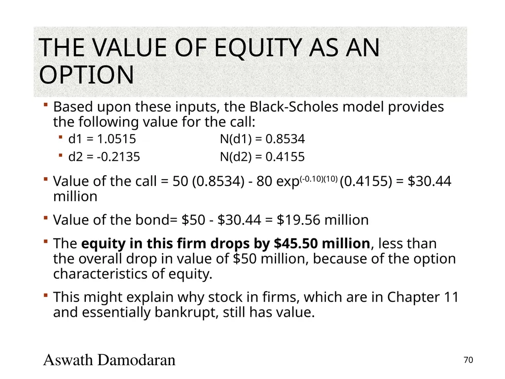
The Value of Equity as an Option Based upon these inputs, the Black-Scholes model provides the following value for the call:
d1 = 1.0515 N(d1) = 0.8534
d2 = -0.2135 N(d2) = 0.4155
Value of the call = 50 (0.8534) - 80 exp(-0.10)(10) (0.4155) = $30.44 million
Value of the bond= $50 - $30.44 = $19.56 million
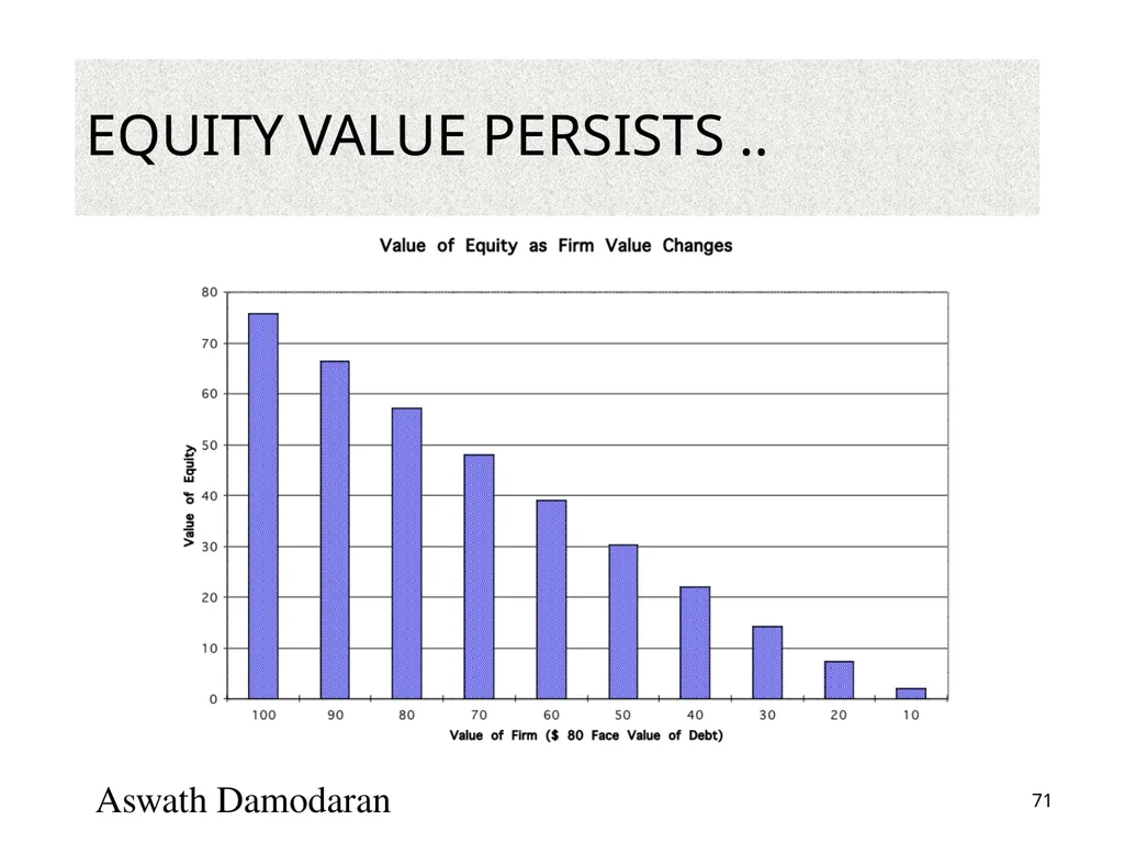
The equity in this firm drops by $45.50 million, less than the overall drop in value of $50 million, because of the option characteristics of equity.
This might explain why stock in firms, which are in Chapter 11 and essentially bankrupt, still has value. Aswath Damodaran 70<br>
d1 = 1.0515 N(d1) = 0.8534
d2 = -0.2135 N(d2) = 0.4155
Value of the call = 50 (0.8534) - 80 exp(-0.10)(10) (0.4155) = $30.44 million
Value of the bond= $50 - $30.44 = $19.56 million
The equity in this firm drops by $45.50 million, less than the overall drop in value of $50 million, because of the option characteristics of equity.
This might explain why stock in firms, which are in Chapter 11 and essentially bankrupt, still has value. Aswath Damodaran 70<br>
71
Equity value persists .. Aswath Damodaran 71<br>
72
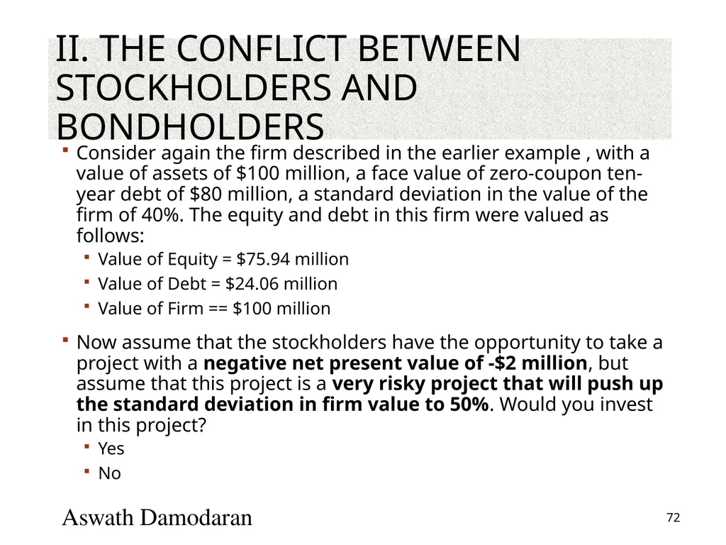
II. The conflict between stockholders and bondholders Consider again the firm described in the earlier example , with a value of assets of $100 million, a face value of zero-coupon ten-year debt of $80 million, a standard deviation in the value of the firm of 40%. The equity and debt in this firm were valued as follows:
Value of Equity = $75.94 million
Value of Debt = $24.06 million
Value of Firm == $100 million
Now assume that the stockholders have the opportunity to take a project with a negative net present value of -$2 million, but assume that this project is a very risky project that will push up the standard deviation in firm value to 50%. Would you invest in this project?
Yes
No Aswath Damodaran 72<br>
Value of Equity = $75.94 million
Value of Debt = $24.06 million
Value of Firm == $100 million
Now assume that the stockholders have the opportunity to take a project with a negative net present value of -$2 million, but assume that this project is a very risky project that will push up the standard deviation in firm value to 50%. Would you invest in this project?
Yes
No Aswath Damodaran 72<br>
73
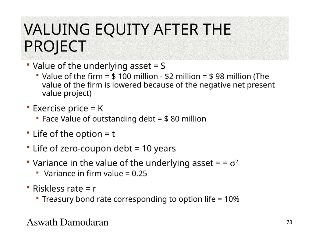
Valuing Equity after the Project Value of the underlying asset = S
Value of the firm = $ 100 million - $2 million = $ 98 million (The value of the firm is lowered because of the negative net present value project)
Exercise price = K
Face Value of outstanding debt = $ 80 million
Life of the option = t
Life of zero-coupon debt = 10 years
Variance in the value of the underlying asset = = s2
Variance in firm value = 0.25
Riskless rate = r
Treasury bond rate corresponding to option life = 10% Aswath Damodaran 73<br>
Value of the firm = $ 100 million - $2 million = $ 98 million (The value of the firm is lowered because of the negative net present value project)
Exercise price = K
Face Value of outstanding debt = $ 80 million
Life of the option = t
Life of zero-coupon debt = 10 years
Variance in the value of the underlying asset = = s2
Variance in firm value = 0.25
Riskless rate = r
Treasury bond rate corresponding to option life = 10% Aswath Damodaran 73<br>
74
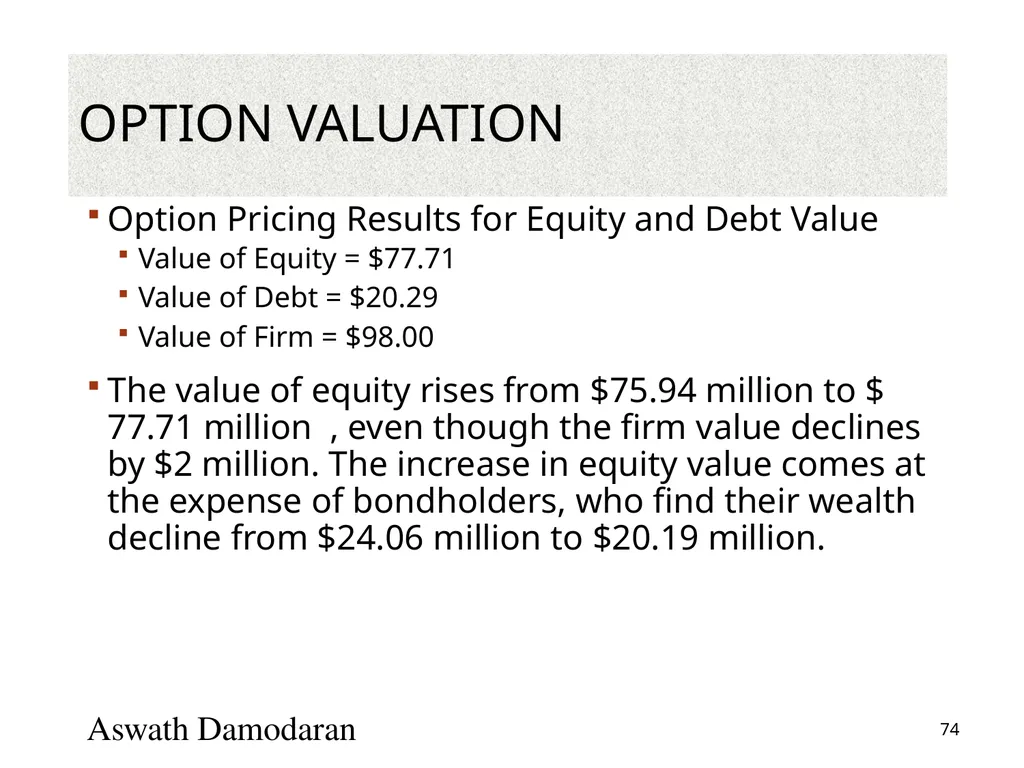
Option Valuation Option Pricing Results for Equity and Debt Value
Value of Equity = $77.71
Value of Debt = $20.29
Value of Firm = $98.00
The value of equity rises from $75.94 million to $ 77.71 million , even though the firm value declines by $2 million. The increase in equity value comes at the expense of bondholders, who find their wealth decline from $24.06 million to $20.19 million. Aswath Damodaran 74<br>
Value of Equity = $77.71
Value of Debt = $20.29
Value of Firm = $98.00
The value of equity rises from $75.94 million to $ 77.71 million , even though the firm value declines by $2 million. The increase in equity value comes at the expense of bondholders, who find their wealth decline from $24.06 million to $20.19 million. Aswath Damodaran 74<br>
75
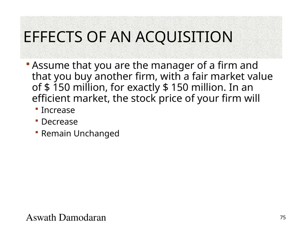
Effects of an Acquisition Assume that you are the manager of a firm and that you buy another firm, with a fair market value of $ 150 million, for exactly $ 150 million. In an efficient market, the stock price of your firm will
Increase
Decrease
Remain Unchanged Aswath Damodaran 75<br>
Increase
Decrease
Remain Unchanged Aswath Damodaran 75<br>
76
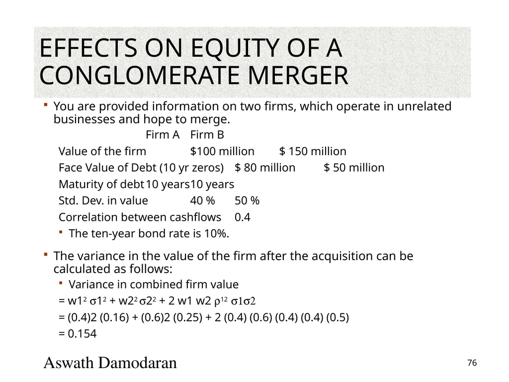
Effects on equity of a conglomerate merger You are provided information on two firms, which operate in unrelated businesses and hope to merge.
Firm A Firm B
Value of the firm $100 million $ 150 million
Face Value of Debt (10 yr zeros) $ 80 million $ 50 million
Maturity of debt 10 years 10 years
Std. Dev. in value 40 % 50 %
Correlation between cashflows 0.4
The ten-year bond rate is 10%.
The variance in the value of the firm after the acquisition can be calculated as follows:
Variance in combined firm value
= w12 s12 + w22 s22 + 2 w1 w2 r12 s1s2
= (0.4)2 (0.16) + (0.6)2 (0.25) + 2 (0.4) (0.6) (0.4) (0.4) (0.5)
= 0.154 Aswath Damodaran 76<br>
Firm A Firm B
Value of the firm $100 million $ 150 million
Face Value of Debt (10 yr zeros) $ 80 million $ 50 million
Maturity of debt 10 years 10 years
Std. Dev. in value 40 % 50 %
Correlation between cashflows 0.4
The ten-year bond rate is 10%.
The variance in the value of the firm after the acquisition can be calculated as follows:
Variance in combined firm value
= w12 s12 + w22 s22 + 2 w1 w2 r12 s1s2
= (0.4)2 (0.16) + (0.6)2 (0.25) + 2 (0.4) (0.6) (0.4) (0.4) (0.5)
= 0.154 Aswath Damodaran 76<br>
77
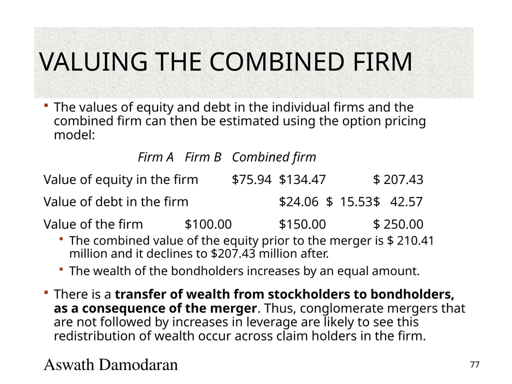
Valuing the Combined Firm The values of equity and debt in the individual firms and the combined firm can then be estimated using the option pricing model:
Firm A Firm B Combined firm
Value of equity in the firm $75.94 $134.47 $ 207.43
Value of debt in the firm $24.06 $ 15.53 $ 42.57
Value of the firm $100.00 $150.00 $ 250.00
The combined value of the equity prior to the merger is $ 210.41 million and it declines to $207.43 million after.
The wealth of the bondholders increases by an equal amount.
There is a transfer of wealth from stockholders to bondholders, as a consequence of the merger. Thus, conglomerate mergers that are not followed by increases in leverage are likely to see this redistribution of wealth occur across claim holders in the firm. Aswath Damodaran 77<br>
Firm A Firm B Combined firm
Value of equity in the firm $75.94 $134.47 $ 207.43
Value of debt in the firm $24.06 $ 15.53 $ 42.57
Value of the firm $100.00 $150.00 $ 250.00
The combined value of the equity prior to the merger is $ 210.41 million and it declines to $207.43 million after.
The wealth of the bondholders increases by an equal amount.
There is a transfer of wealth from stockholders to bondholders, as a consequence of the merger. Thus, conglomerate mergers that are not followed by increases in leverage are likely to see this redistribution of wealth occur across claim holders in the firm. Aswath Damodaran 77<br>
78
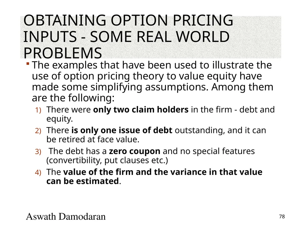
Obtaining option pricing inputs - Some real world problems The examples that have been used to illustrate the use of option pricing theory to value equity have made some simplifying assumptions. Among them are the following:
There were only two claim holders in the firm - debt and equity.
There is only one issue of debt outstanding, and it can be retired at face value.
The debt has a zero coupon and no special features (convertibility, put clauses etc.)
The value of the firm and the variance in that value can be estimated. Aswath Damodaran 78<br>
There were only two claim holders in the firm - debt and equity.
There is only one issue of debt outstanding, and it can be retired at face value.
The debt has a zero coupon and no special features (convertibility, put clauses etc.)
The value of the firm and the variance in that value can be estimated. Aswath Damodaran 78<br>
79
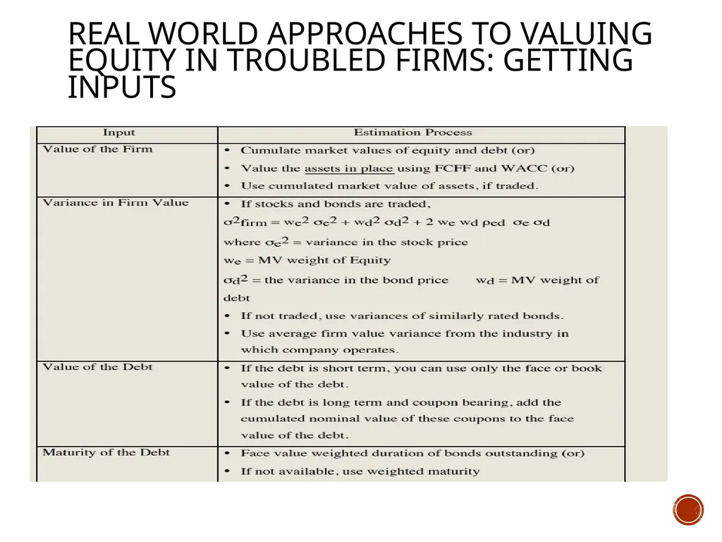
Real World Approaches to Valuing Equity in Troubled Firms: Getting Inputs<br>
80
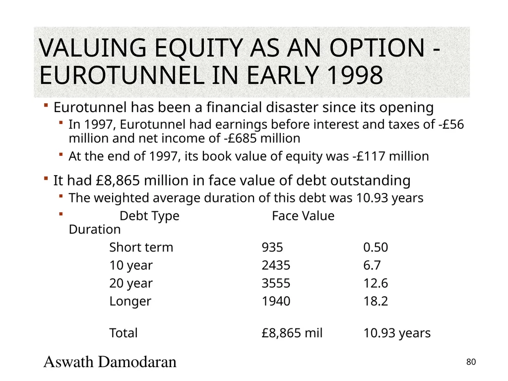
Valuing Equity as an option - Eurotunnel in early 1998 Eurotunnel has been a financial disaster since its opening
In 1997, Eurotunnel had earnings before interest and taxes of -£56 million and net income of -£685 million
At the end of 1997, its book value of equity was -£117 million
It had £8,865 million in face value of debt outstanding
The weighted average duration of this debt was 10.93 years
Debt Type Face Value Duration
Short term 935 0.50
10 year 2435 6.7
20 year 3555 12.6
Longer 1940 18.2
Total £8,865 mil 10.93 years Aswath Damodaran 80<br>
In 1997, Eurotunnel had earnings before interest and taxes of -£56 million and net income of -£685 million
At the end of 1997, its book value of equity was -£117 million
It had £8,865 million in face value of debt outstanding
The weighted average duration of this debt was 10.93 years
Debt Type Face Value Duration
Short term 935 0.50
10 year 2435 6.7
20 year 3555 12.6
Longer 1940 18.2
Total £8,865 mil 10.93 years Aswath Damodaran 80<br>
81
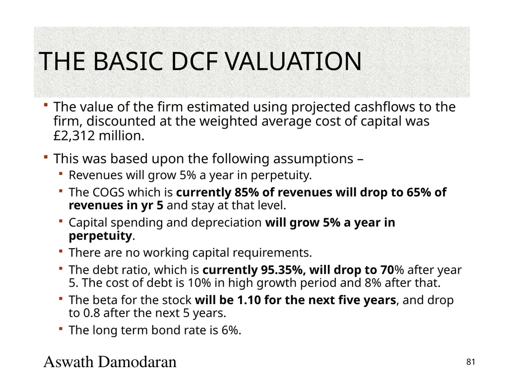
The Basic DCF Valuation The value of the firm estimated using projected cashflows to the firm, discounted at the weighted average cost of capital was £2,312 million.
This was based upon the following assumptions –
Revenues will grow 5% a year in perpetuity.
The COGS which is currently 85% of revenues will drop to 65% of revenues in yr 5 and stay at that level.
Capital spending and depreciation will grow 5% a year in perpetuity.
There are no working capital requirements.
The debt ratio, which is currently 95.35%, will drop to 70% after year 5. The cost of debt is 10% in high growth period and 8% after that.
The beta for the stock will be 1.10 for the next five years, and drop to 0.8 after the next 5 years.
The long term bond rate is 6%. Aswath Damodaran 81<br>
This was based upon the following assumptions –
Revenues will grow 5% a year in perpetuity.
The COGS which is currently 85% of revenues will drop to 65% of revenues in yr 5 and stay at that level.
Capital spending and depreciation will grow 5% a year in perpetuity.
There are no working capital requirements.
The debt ratio, which is currently 95.35%, will drop to 70% after year 5. The cost of debt is 10% in high growth period and 8% after that.
The beta for the stock will be 1.10 for the next five years, and drop to 0.8 after the next 5 years.
The long term bond rate is 6%. Aswath Damodaran 81<br>
82
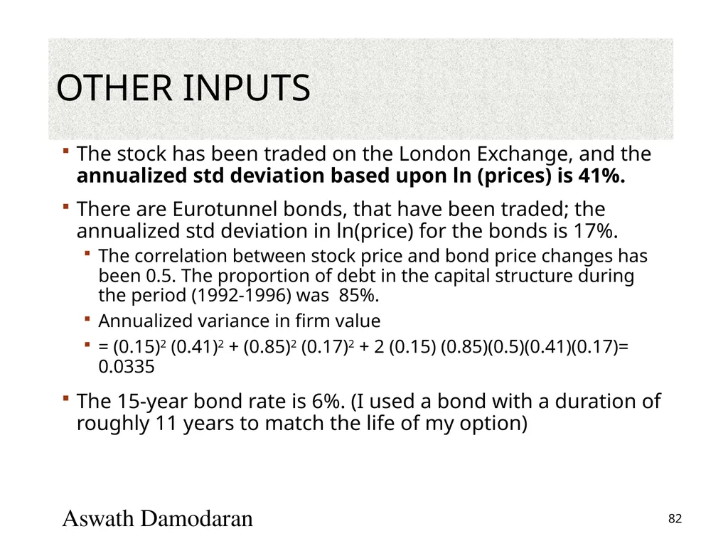
Other Inputs The stock has been traded on the London Exchange, and the annualized std deviation based upon ln (prices) is 41%.
There are Eurotunnel bonds, that have been traded; the annualized std deviation in ln(price) for the bonds is 17%.
The correlation between stock price and bond price changes has been 0.5. The proportion of debt in the capital structure during the period (1992-1996) was 85%.
Annualized variance in firm value
= (0.15)2 (0.41)2 + (0.85)2 (0.17)2 + 2 (0.15) (0.85)(0.5)(0.41)(0.17)= 0.0335
The 15-year bond rate is 6%. (I used a bond with a duration of roughly 11 years to match the life of my option) Aswath Damodaran 82<br>
There are Eurotunnel bonds, that have been traded; the annualized std deviation in ln(price) for the bonds is 17%.
The correlation between stock price and bond price changes has been 0.5. The proportion of debt in the capital structure during the period (1992-1996) was 85%.
Annualized variance in firm value
= (0.15)2 (0.41)2 + (0.85)2 (0.17)2 + 2 (0.15) (0.85)(0.5)(0.41)(0.17)= 0.0335
The 15-year bond rate is 6%. (I used a bond with a duration of roughly 11 years to match the life of my option) Aswath Damodaran 82<br>
83
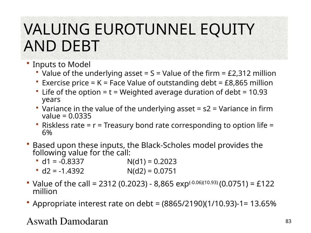
Valuing Eurotunnel Equity and Debt Inputs to Model
Value of the underlying asset = S = Value of the firm = £2,312 million
Exercise price = K = Face Value of outstanding debt = £8,865 million
Life of the option = t = Weighted average duration of debt = 10.93 years
Variance in the value of the underlying asset = s2 = Variance in firm value = 0.0335
Riskless rate = r = Treasury bond rate corresponding to option life = 6%
Based upon these inputs, the Black-Scholes model provides the following value for the call:
d1 = -0.8337 N(d1) = 0.2023
d2 = -1.4392 N(d2) = 0.0751
Value of the call = 2312 (0.2023) - 8,865 exp(-0.06)(10.93) (0.0751) = £122 million
Appropriate interest rate on debt = (8865/2190)(1/10.93)-1= 13.65% Aswath Damodaran 83<br>
Value of the underlying asset = S = Value of the firm = £2,312 million
Exercise price = K = Face Value of outstanding debt = £8,865 million
Life of the option = t = Weighted average duration of debt = 10.93 years
Variance in the value of the underlying asset = s2 = Variance in firm value = 0.0335
Riskless rate = r = Treasury bond rate corresponding to option life = 6%
Based upon these inputs, the Black-Scholes model provides the following value for the call:
d1 = -0.8337 N(d1) = 0.2023
d2 = -1.4392 N(d2) = 0.0751
Value of the call = 2312 (0.2023) - 8,865 exp(-0.06)(10.93) (0.0751) = £122 million
Appropriate interest rate on debt = (8865/2190)(1/10.93)-1= 13.65% Aswath Damodaran 83<br>
84
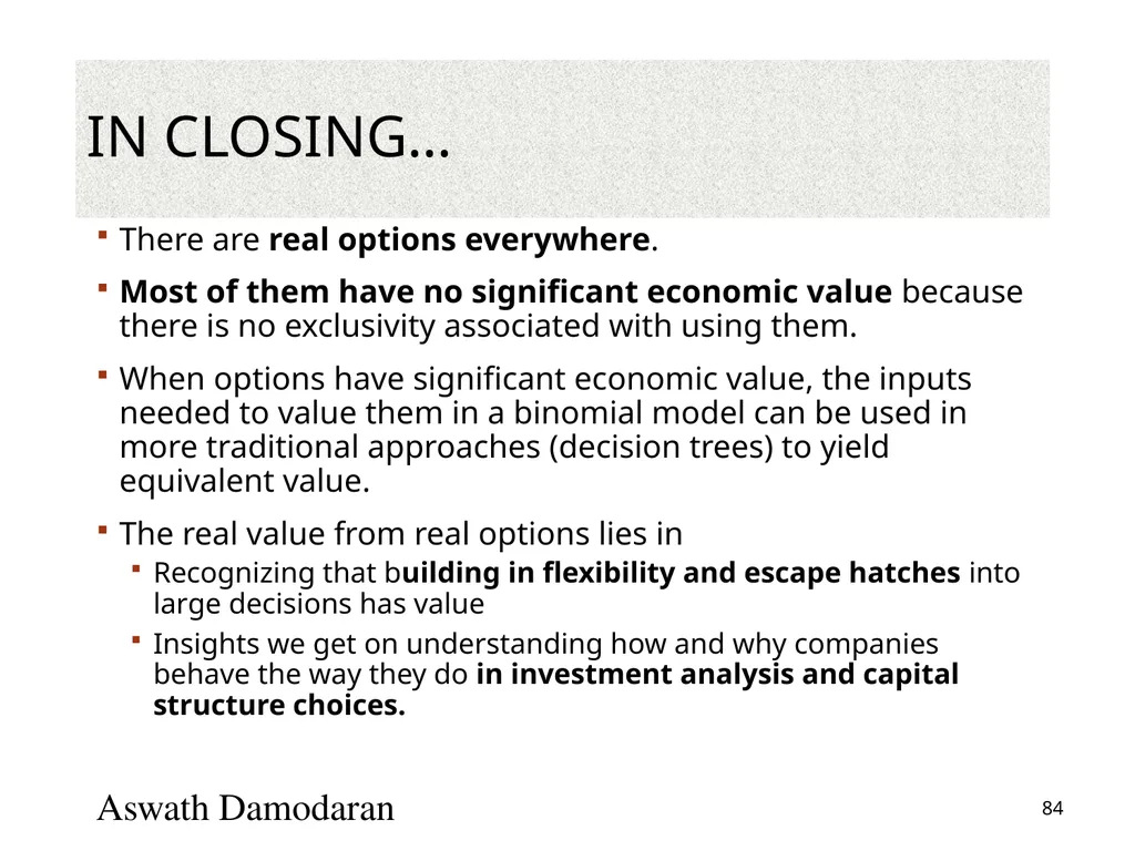
In Closing… There are real options everywhere.
Most of them have no significant economic value because there is no exclusivity associated with using them.
When options have significant economic value, the inputs needed to value them in a binomial model can be used in more traditional approaches (decision trees) to yield equivalent value.
The real value from real options lies in
Recognizing that building in flexibility and escape hatches into large decisions has value
Insights we get on understanding how and why companies behave the way they do in investment analysis and capital structure choices. Aswath Damodaran 84<br>
Most of them have no significant economic value because there is no exclusivity associated with using them.
When options have significant economic value, the inputs needed to value them in a binomial model can be used in more traditional approaches (decision trees) to yield equivalent value.
The real value from real options lies in
Recognizing that building in flexibility and escape hatches into large decisions has value
Insights we get on understanding how and why companies behave the way they do in investment analysis and capital structure choices. Aswath Damodaran 84<br>
85
Acquirers Anonymous: Seven Steps back to Sobriety… Aswath Damodaran 85<br>
86
Great for target companies but not for acquiring company stockholders… Aswath Damodaran 86<br>
87
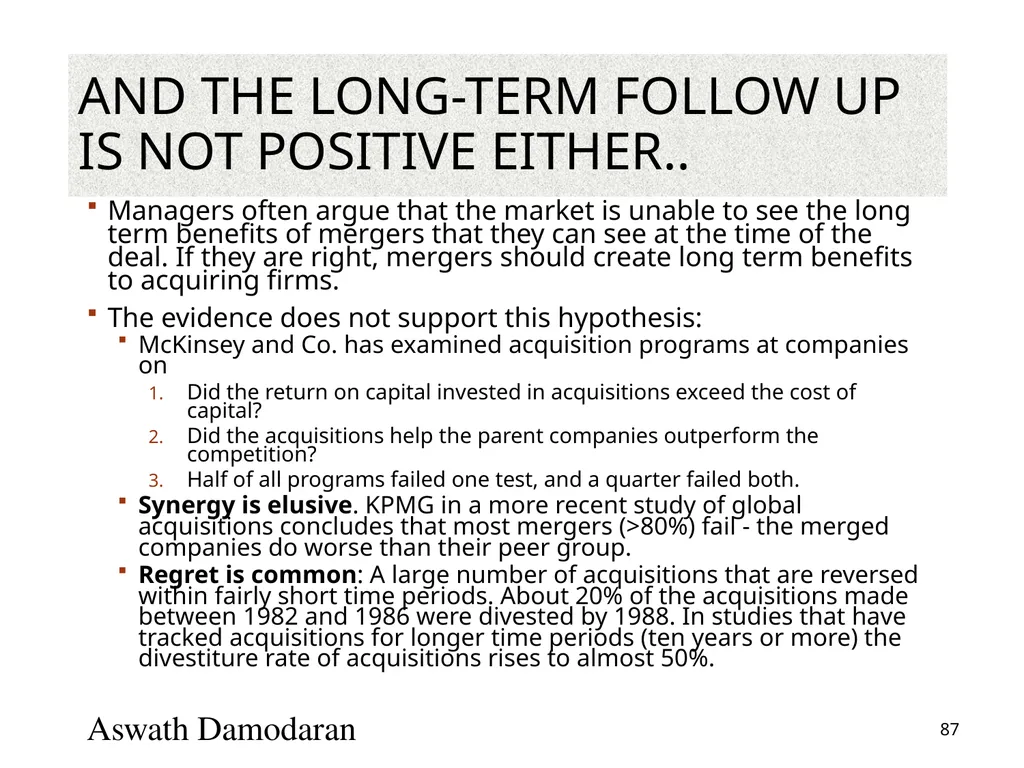
And the long-term follow up is not positive either.. Managers often argue that the market is unable to see the long term benefits of mergers that they can see at the time of the deal. If they are right, mergers should create long term benefits to acquiring firms.
The evidence does not support this hypothesis:
McKinsey and Co. has examined acquisition programs at companies on
Did the return on capital invested in acquisitions exceed the cost of capital?
Did the acquisitions help the parent companies outperform the competition?
Half of all programs failed one test, and a quarter failed both.
Synergy is elusive. KPMG in a more recent study of global acquisitions concludes that most mergers (>80%) fail - the merged companies do worse than their peer group.
Regret is common: A large number of acquisitions that are reversed within fairly short time periods. About 20% of the acquisitions made between 1982 and 1986 were divested by 1988. In studies that have tracked acquisitions for longer time periods (ten years or more) the divestiture rate of acquisitions rises to almost 50%. Aswath Damodaran 87<br>
The evidence does not support this hypothesis:
McKinsey and Co. has examined acquisition programs at companies on
Did the return on capital invested in acquisitions exceed the cost of capital?
Did the acquisitions help the parent companies outperform the competition?
Half of all programs failed one test, and a quarter failed both.
Synergy is elusive. KPMG in a more recent study of global acquisitions concludes that most mergers (>80%) fail - the merged companies do worse than their peer group.
Regret is common: A large number of acquisitions that are reversed within fairly short time periods. About 20% of the acquisitions made between 1982 and 1986 were divested by 1988. In studies that have tracked acquisitions for longer time periods (ten years or more) the divestiture rate of acquisitions rises to almost 50%. Aswath Damodaran 87<br>
88
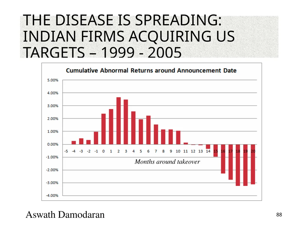
The disease is spreading: Indian firms acquiring US targets – 1999 - 2005 Aswath Damodaran 88 Months around takeover<br>
89
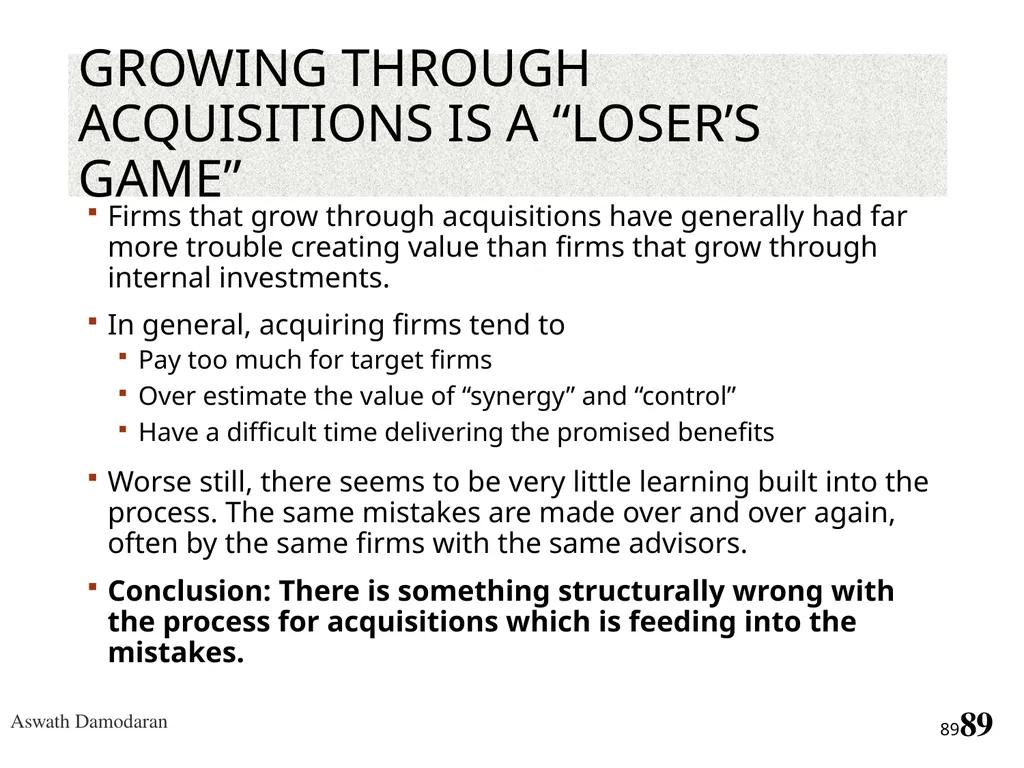
Growing through acquisitions is a “loser’s game” Firms that grow through acquisitions have generally had far more trouble creating value than firms that grow through internal investments.
In general, acquiring firms tend to
Pay too much for target firms
Over estimate the value of “synergy” and “control”
Have a difficult time delivering the promised benefits
Worse still, there seems to be very little learning built into the process. The same mistakes are made over and over again, often by the same firms with the same advisors.
Conclusion: There is something structurally wrong with the process for acquisitions which is feeding into the mistakes. 89 Aswath Damodaran<br>
In general, acquiring firms tend to
Pay too much for target firms
Over estimate the value of “synergy” and “control”
Have a difficult time delivering the promised benefits
Worse still, there seems to be very little learning built into the process. The same mistakes are made over and over again, often by the same firms with the same advisors.
Conclusion: There is something structurally wrong with the process for acquisitions which is feeding into the mistakes. 89 Aswath Damodaran<br>
90
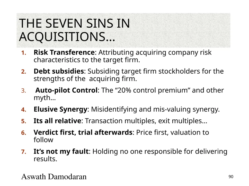
The seven sins in acquisitions… Risk Transference: Attributing acquiring company risk characteristics to the target firm.
Debt subsidies: Subsiding target firm stockholders for the strengths of the acquiring firm.
Auto-pilot Control: The “20% control premium” and other myth…
Elusive Synergy: Misidentifying and mis-valuing synergy.
Its all relative: Transaction multiples, exit multiples…
Verdict first, trial afterwards: Price first, valuation to follow
It’s not my fault: Holding no one responsible for delivering results. Aswath Damodaran 90<br>
Debt subsidies: Subsiding target firm stockholders for the strengths of the acquiring firm.
Auto-pilot Control: The “20% control premium” and other myth…
Elusive Synergy: Misidentifying and mis-valuing synergy.
Its all relative: Transaction multiples, exit multiples…
Verdict first, trial afterwards: Price first, valuation to follow
It’s not my fault: Holding no one responsible for delivering results. Aswath Damodaran 90<br>
91
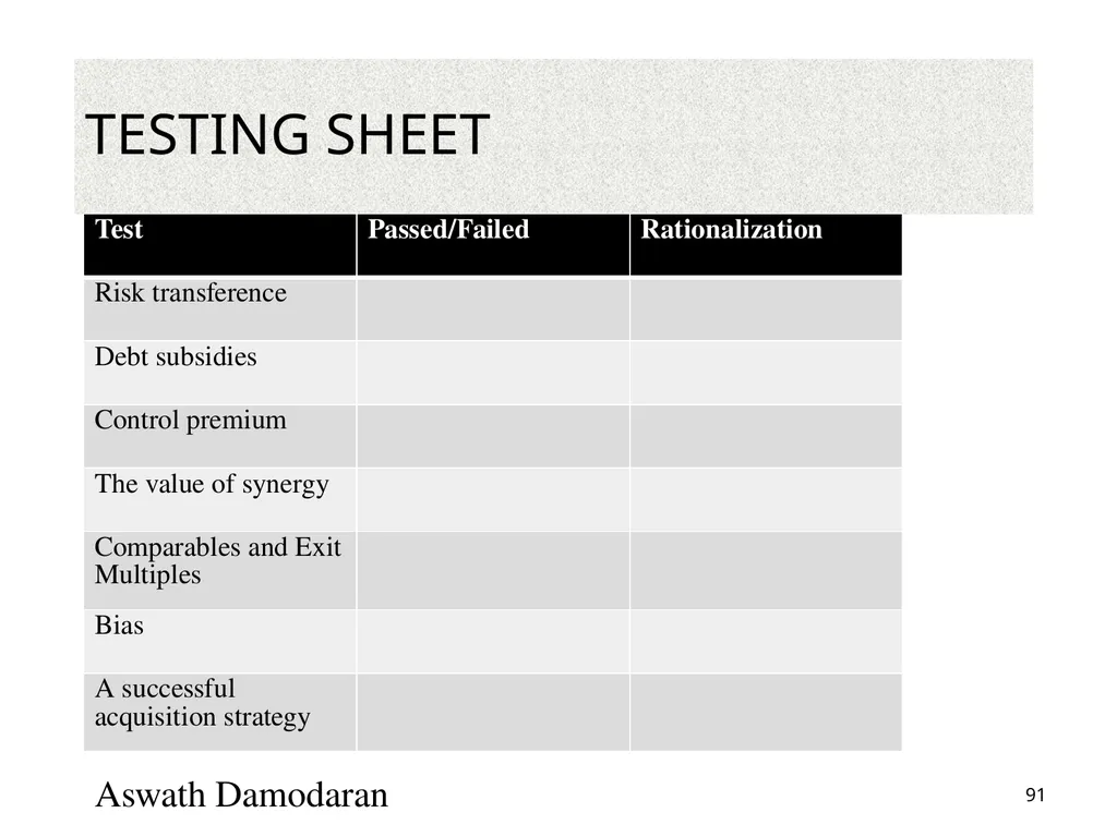
Testing sheet Aswath Damodaran 91<br>
92
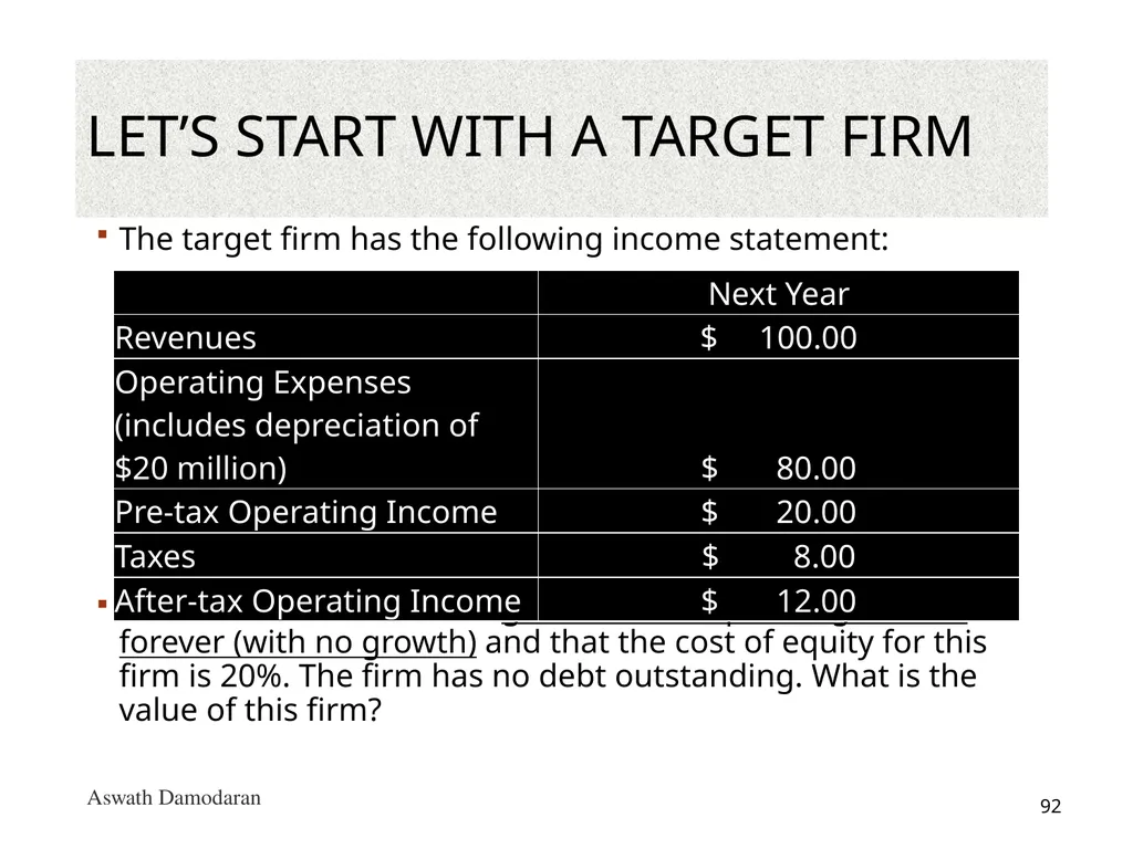
Let’s start with a target firm The target firm has the following income statement:
Assume that this firm will generate this operating income forever (with no growth) and that the cost of equity for this firm is 20%. The firm has no debt outstanding. What is the value of this firm? Aswath Damodaran 92<br>
Assume that this firm will generate this operating income forever (with no growth) and that the cost of equity for this firm is 20%. The firm has no debt outstanding. What is the value of this firm? Aswath Damodaran 92<br>
93
Test 1: Risk Transference… Assume that as an acquiring firm, you are in a much safer business and have a cost of equity of 10%. What is the value of the target firm to you?
$60 million
$90 million
$120 million
Other 93 Aswath Damodaran<br>
$60 million
$90 million
$120 million
Other 93 Aswath Damodaran<br>
94
Lesson 1: Don’t transfer your risk characteristics to the target firm Let’s start with a basic capital budgeting principle, which is often ignored: The discount rate used for an investment should reflect the risk of the investment and not the risk characteristics of the investor who raised the funds.
Risky businesses cannot become safe just because the buyer of these businesses is in a safe business.
The right cost of equity to use in valuation is the one that reflects the risk in equity in the target firm. 94 Aswath Damodaran<br>
Risky businesses cannot become safe just because the buyer of these businesses is in a safe business.
The right cost of equity to use in valuation is the one that reflects the risk in equity in the target firm. 94 Aswath Damodaran<br>
95
Test 2: Cheap debt? Assume as an acquirer that you have both excess debt capacity (because you have not chosen to borrow as much as you could have, given your assets) and access to cheap debt.
You plan to borrow money at 4% (in after-tax terms) and that you plan to fund half the acquisition with debt. How much would you be willing to pay for the target firm? Aswath Damodaran 95<br>
You plan to borrow money at 4% (in after-tax terms) and that you plan to fund half the acquisition with debt. How much would you be willing to pay for the target firm? Aswath Damodaran 95<br>
96
Lesson 2: Render unto the target firm that which is the target firm’s but not a penny more.. As an acquiring firm, it is entirely possible that you can borrow much more than the target firm can on its own and at a much lower rate.
If you build these characteristics into the valuation of the target firm, you are essentially transferring wealth from your firm’s stockholder to the target firm’s stockholders.
When valuing a target firm, use a cost of capital that reflects the debt capacity and the cost of debt that would apply to the firm. Aswath Damodaran 96<br>
If you build these characteristics into the valuation of the target firm, you are essentially transferring wealth from your firm’s stockholder to the target firm’s stockholders.
When valuing a target firm, use a cost of capital that reflects the debt capacity and the cost of debt that would apply to the firm. Aswath Damodaran 96<br>
97
Test 3: Control Premiums Assume that you are now told that it is conventional to pay a 20% premium for control in acquisitions.
That premium is justified by pointing to historical studies that show that this is what acquirers pay for control, i.e., pay roughly a 20% premium over the market price.
How much would you be willing to pay for the target firm?
Assuming that you are paying a control premium, how would you justify it? Aswath Damodaran 97<br>
That premium is justified by pointing to historical studies that show that this is what acquirers pay for control, i.e., pay roughly a 20% premium over the market price.
How much would you be willing to pay for the target firm?
Assuming that you are paying a control premium, how would you justify it? Aswath Damodaran 97<br>
98
Lesson 3: Beware of rules of thumb… Valuation is cluttered with rules of thumb. After painstakingly valuing a target firm, using your best estimates, you will be often be told that
It is common practice to add arbitrary premiums for brand name, quality of management, control etc…
These premiums will be often be backed up by data, studies and services. What they will not reveal is the enormous sampling bias in the studies and the standard errors in the estimates.
If you have done your valuation right, those premiums should already be incorporated in your estimated value. Paying a premium will be double counting. Aswath Damodaran 98<br>
It is common practice to add arbitrary premiums for brand name, quality of management, control etc…
These premiums will be often be backed up by data, studies and services. What they will not reveal is the enormous sampling bias in the studies and the standard errors in the estimates.
If you have done your valuation right, those premiums should already be incorporated in your estimated value. Paying a premium will be double counting. Aswath Damodaran 98<br>
99
Test 4: Synergy…. Assume that you are told that the combined firm will be less risky than the two individual firms and that it should have a lower cost of capital (and a higher value). Is this likely?
Yes
No
Assume now that you are told that there are potential growth and cost savings synergies in the acquisition. Would that constitute value added?
Yes
No
Should you pay this as a premium?
Yes
No Aswath Damodaran 99<br>
Yes
No
Assume now that you are told that there are potential growth and cost savings synergies in the acquisition. Would that constitute value added?
Yes
No
Should you pay this as a premium?
Yes
No Aswath Damodaran 99<br>
100
The Value of Synergy Aswath Damodaran 100<br>
101
Valuing Synergy (1) the firms involved in the merger are valued independently, by discounting expected cash flows to each firm at the weighted average cost of capital for that firm.
(2) the value of the combined firm, with no synergy, is obtained by adding the values obtained for each firm in the first step.
(3) The effects of synergy are built into expected growth rates and cashflows, and the combined firm is re-valued with synergy.
Value of Synergy = Value of the combined firm, with synergy - Value of the combined firm, without synergy Aswath Damodaran 101<br>
(2) the value of the combined firm, with no synergy, is obtained by adding the values obtained for each firm in the first step.
(3) The effects of synergy are built into expected growth rates and cashflows, and the combined firm is re-valued with synergy.
Value of Synergy = Value of the combined firm, with synergy - Value of the combined firm, without synergy Aswath Damodaran 101<br>
102
Synergy - Example 1
Higher growth and cost savings Aswath Damodaran 102<br>
103
Synergy: Example 2
Tax Benefits? Assume that you are Best Buy, the electronics retailer, and that you would like to enter the hardware component of the market. You have been approached by investment bankers for Zenith, which while still a recognized brand name, is on its last legs financially. The firm has net operating losses of $ 2 billion. If your tax rate is 36%, estimate the tax benefits from this acquisition.
If Best Buy had only $500 million in taxable income, how would you compute the tax benefits?
If the market value of Zenith is $800 million, would you pay this tax benefit as a premium on the market value? Aswath Damodaran 103<br>
If Best Buy had only $500 million in taxable income, how would you compute the tax benefits?
If the market value of Zenith is $800 million, would you pay this tax benefit as a premium on the market value? Aswath Damodaran 103<br>
104
Lesson 4: Don’t pay for buzz words You have to value synergy, before you decide how much to pay (not after): Synergy will be the buzzword that explains away the premium that you are paying.
To value synergy, you need specifics: Before you value synergy, you need to be specific about what synergies you see in a merger and where they will show up in a valuation.
Don’t mistake control for synergy: If the benefits can be generated by just one of the two entities in the merger, it is not synergy.
Negotiate for your fair share: As the acquiring firm, you should negotiate for your share of the synergy, not pay it all off as a premium. Aswath Damodaran 104<br>
To value synergy, you need specifics: Before you value synergy, you need to be specific about what synergies you see in a merger and where they will show up in a valuation.
Don’t mistake control for synergy: If the benefits can be generated by just one of the two entities in the merger, it is not synergy.
Negotiate for your fair share: As the acquiring firm, you should negotiate for your share of the synergy, not pay it all off as a premium. Aswath Damodaran 104<br>
105
Test 5: Comparables and Exit Multiples Now assume that you are told that an analysis of other acquisitions reveals that acquirers have been willing to pay 5 times EBIT.. Given that your target firm has EBIT of $ 20 million, would you be willing to pay $ 100 million for the acquisition?
What if I estimate the terminal value using an exit multiple of 5 times EBIT?
As an additional input, your investment banker tells you that the acquisition is accretive. (Your PE ratio is 20 whereas the PE ratio of the target is only 10… Therefore, you will get a jump in earnings per share after the acquisition…) Aswath Damodaran 105<br>
What if I estimate the terminal value using an exit multiple of 5 times EBIT?
As an additional input, your investment banker tells you that the acquisition is accretive. (Your PE ratio is 20 whereas the PE ratio of the target is only 10… Therefore, you will get a jump in earnings per share after the acquisition…) Aswath Damodaran 105<br>
106
Biased samples = Poor results Biased samples yield biased results. Basing what you pay on what other acquirers have paid is a recipe for disaster. After all, we know that acquirer, on average, pay too much for acquisitions. By matching their prices, we risk replicating their mistakes.
Even when we use the pricing metrics of other firms in the sector, we may be basing the prices we pay on firms that are not truly comparable.
When we use exit multiples, we are assuming that what the market is paying for comparable companies today is what it will continue to pay in the future. Aswath Damodaran 106<br>
Even when we use the pricing metrics of other firms in the sector, we may be basing the prices we pay on firms that are not truly comparable.
When we use exit multiples, we are assuming that what the market is paying for comparable companies today is what it will continue to pay in the future. Aswath Damodaran 106<br>
107
Lesson 5: If you are going to price a target firm, do it right.. Pick your game: If you are acquiring other companies not for the cash flows but because you think that you can sell them to someone else at a higher price, it is perfectly okay to play the pricing game. If you are acquiring a firm for its cash flows, you have to play the value game.
Don’t get distracted: If you are playing the pricing game, dispense with the DCF and do an honest pricing. If you are playing the value game, stop looking at what other people are paying.
To do an honest pricing, you have to be unbiased in your choice of multiple and comparable firms, and control for differences between your firm & the peer group. 107 Aswath Damodaran<br>
Don’t get distracted: If you are playing the pricing game, dispense with the DCF and do an honest pricing. If you are playing the value game, stop looking at what other people are paying.
To do an honest pricing, you have to be unbiased in your choice of multiple and comparable firms, and control for differences between your firm & the peer group. 107 Aswath Damodaran<br>
108
Test 6: The CEO really wants to do this… or there are competitive pressures… Now assume that you know that the CEO of the acquiring firm really, really wants to do this acquisition and that the investment bankers on both sides have produced fairness opinions that indicate that the firm is worth $ 150 million. Would you be willing to go along?
Yes
No
Now assume that you are told that your competitors are all doing acquisitions and that if you don’t do them, you will be at a disadvantage? Would you be willing to go along?
Yes
No Aswath Damodaran 108<br>
Yes
No
Now assume that you are told that your competitors are all doing acquisitions and that if you don’t do them, you will be at a disadvantage? Would you be willing to go along?
Yes
No Aswath Damodaran 108<br>
109
CEO Egos and Overconfidence: The Dirty Secret in Mergers The Deal Rules: The premiums paid on acquisitions often have nothing to do with synergy, control or strategic considerations (though they may be provided as the reasons). They are just what you have to pay to get the deals done, because management really, really wants it done.
The Ego Problem: They may just reflect the egos of the CEOs of the acquiring firms. There is evidence that “over confident” CEOs are more likely to make acquisitions and that they leave a trail across the firms that they run. 109 Aswath Damodaran<br>
The Ego Problem: They may just reflect the egos of the CEOs of the acquiring firms. There is evidence that “over confident” CEOs are more likely to make acquisitions and that they leave a trail across the firms that they run. 109 Aswath Damodaran<br>
110
Defensive Mergers: Signs of a Deeper Rot? Me-tooism: Pre-emptive or defensive acquisitions, where you over pay, either because everyone else is overpaying or because you are afraid that you will be left behind if you don’t acquire are dangerous.
Weak businesses? If the only way you can stay competitive in a business is by making bad investments, it may be best to think about shrinking or even getting out of the business.
There is no glory in survival, for the sake of survival. Corporate sustainability, as a corporate objective, is not just a joke, but an expensive one. 110 Aswath Damodaran<br>
Weak businesses? If the only way you can stay competitive in a business is by making bad investments, it may be best to think about shrinking or even getting out of the business.
There is no glory in survival, for the sake of survival. Corporate sustainability, as a corporate objective, is not just a joke, but an expensive one. 110 Aswath Damodaran<br>
111
Lesson 6: Don’t let egos or investment bankers get the better of common sense… If you define your objective in a bidding war as winning the auction at any cost, you will win. But beware the winner’s curse!
The premiums paid on acquisitions often have nothing to do with synergy, control or strategic considerations. They may just reflect the egos of the CEOs of the acquiring firms. There is evidence that “overconfident” CEOs are more likely to make acquisitions and that they leave a trail across the firms that they run.
Pre-emptive or defensive acquisitions, where you over pay, either because everyone else is overpaying or because you are afraid that you will be left behind if you don’t acquire are dangerous. If the only way you can stay competitive in a business is by making bad investments, it may be best to think about getting out of the business. Aswath Damodaran 111<br>
The premiums paid on acquisitions often have nothing to do with synergy, control or strategic considerations. They may just reflect the egos of the CEOs of the acquiring firms. There is evidence that “overconfident” CEOs are more likely to make acquisitions and that they leave a trail across the firms that they run.
Pre-emptive or defensive acquisitions, where you over pay, either because everyone else is overpaying or because you are afraid that you will be left behind if you don’t acquire are dangerous. If the only way you can stay competitive in a business is by making bad investments, it may be best to think about getting out of the business. Aswath Damodaran 111<br>
112
Test 7: When deals fall apart.. When deals fall apart, as many do, there seems to be little or no accountability in the system, and the larger the deal, the less accountability there is for mistakes.
Breaking it down:
The managers who initiate these bad deals seem to face few consequences and often move up the ranks.
The boards that okay these deals protect themselves by claiming that the did due diligence and listened to experts.
The bankers keep their fees, arguing that their missed forecasts were just mistakes. Aswath Damodaran 112<br>
Breaking it down:
The managers who initiate these bad deals seem to face few consequences and often move up the ranks.
The boards that okay these deals protect themselves by claiming that the did due diligence and listened to experts.
The bankers keep their fees, arguing that their missed forecasts were just mistakes. Aswath Damodaran 112<br>
113
To illustrate: A bad deal is made, and justified by accountants & bankers! Aswath Damodaran<br>
114
The CEO steps in… and digs a hole… Leo Apotheker was the CEO of HP at the time of the deal, brought in to replace Mark Hurd, the previous CEO who was forced to resign because of a “sex” scandal.
In the face of almost universal feeling that HP had paid too much for Autonomy, Mr. Apotheker addressing a conference at the time of the deal: “We have a pretty rigorous process inside H.P. that we follow for all our acquisitions, which is a D.C.F.-based model,” he said, in a reference to discounted cash flow, a standard valuation methodology. “And we try to take a very conservative view.”
Apotheker added, “Just to make sure everybody understands, Autonomy will be, on Day 1, accretive to H.P….. “Just take it from us. We did that analysis at great length, in great detail, and we feel that we paid a very fair price for Autonomy. And it will give a great return to our shareholders. Aswath Damodaran 114<br>
In the face of almost universal feeling that HP had paid too much for Autonomy, Mr. Apotheker addressing a conference at the time of the deal: “We have a pretty rigorous process inside H.P. that we follow for all our acquisitions, which is a D.C.F.-based model,” he said, in a reference to discounted cash flow, a standard valuation methodology. “And we try to take a very conservative view.”
Apotheker added, “Just to make sure everybody understands, Autonomy will be, on Day 1, accretive to H.P….. “Just take it from us. We did that analysis at great length, in great detail, and we feel that we paid a very fair price for Autonomy. And it will give a great return to our shareholders. Aswath Damodaran 114<br>
115
A year later… HP admits a mistake…and explains it…<br>
116
A Measured assessment: Is it hopeless? The odds seem to be clearly weighted against success in acquisitions. If you were to create a strategy to grow, based upon acquisitions, which of the following offers your best chance of success? Aswath Damodaran 116<br>
117
Better to lose a bidding war than to win one… Aswath Damodaran 117 Returns in the 40 months before & after bidding war
Source: Malmendier, Moretti & Peters (2011)<br>
Source: Malmendier, Moretti & Peters (2011)<br>
118
Better off buying small rather than large targets… with cash rather than stock Aswath Damodaran 118<br>
119
And focusing on private firms and subsidiaries, rather than public firms… Aswath Damodaran 119<br>
120
Growth vs Cost Synergies Aswath Damodaran 120<br>
121
The Bottom line: For acquisitions to create value, you have to stay disciplined.. If you have a successful acquisition strategy, stay focused on that strategy. Don’t let size or hubris drive you to “expand” the strategy.
Realistic plans for delivering synergy and control have to be put in place before the merger is completed. By realistic, we have to mean that the magnitude of the benefits have to be reachable and not pipe dreams and that the time frame should reflect the reality that it takes a while for two organizations to work as one.
The best thing to do in a bidding war is to drop out.
Someone (preferably the person pushing hardest for the merger) should be held to account for delivering the benefits.
The compensation for investment bankers and others involved in the deal should be tied to how well the deal works rather than for getting the deal done. Aswath Damodaran 121<br>
Realistic plans for delivering synergy and control have to be put in place before the merger is completed. By realistic, we have to mean that the magnitude of the benefits have to be reachable and not pipe dreams and that the time frame should reflect the reality that it takes a while for two organizations to work as one.
The best thing to do in a bidding war is to drop out.
Someone (preferably the person pushing hardest for the merger) should be held to account for delivering the benefits.
The compensation for investment bankers and others involved in the deal should be tied to how well the deal works rather than for getting the deal done. Aswath Damodaran 121<br>
122
Value Enhancement and the Expected Value of Control: Back to Basics Aswath Damodaran 122<br>
123
Price Enhancement versus Value Enhancement Aswath Damodaran 123 The market gives… And takes away….<br>
124
The Paths to Value Creation Using the DCF framework, there are four basic ways in which the value of a firm can be enhanced:
The cash flows from existing assets to the firm can be increased, by either
increasing after-tax earnings from assets in place or
reducing reinvestment needs (net capital expenditures or working capital)
The value from growth in these cash flows can be increased by either
Reinvesting more and increasing growth in good businesses
Reinvesting less or even divesting in bad businesses
The length of the high growth period can be extended to allow for more years of high growth.
The cost of capital can be reduced by
Reducing the operating risk in investments/assets
Changing the financial mix
Changing the financing composition Aswath Damodaran 124<br>
The cash flows from existing assets to the firm can be increased, by either
increasing after-tax earnings from assets in place or
reducing reinvestment needs (net capital expenditures or working capital)
The value from growth in these cash flows can be increased by either
Reinvesting more and increasing growth in good businesses
Reinvesting less or even divesting in bad businesses
The length of the high growth period can be extended to allow for more years of high growth.
The cost of capital can be reduced by
Reducing the operating risk in investments/assets
Changing the financial mix
Changing the financing composition Aswath Damodaran 124<br>
125
Value Creation 1: Increase Cash Flows from Assets in Place Aswath Damodaran 125<br>
126
Divest, Abandon or Hold on: The Math! The conventional wisdom, when you are put in charge of a troubled firm, is to sell or abandon the worst-performing assets, usually ones that earn less than the cost of capital.
Every asset/business that a company owns has three values:
Continuation value: the value of the expected cash flows from continuing to own and operate the asset
Abandonment value: the salvage value of the asset or assets in the business
Divestiture value: the value that the best buyer will pay for the asset or business.
For value enhancement, you pick the highest of the three values, and ironically, the ones that you may most benefit from divesting are your best-regarded, rather than your worst performing, assets. Aswath Damodaran 126<br>
Every asset/business that a company owns has three values:
Continuation value: the value of the expected cash flows from continuing to own and operate the asset
Abandonment value: the salvage value of the asset or assets in the business
Divestiture value: the value that the best buyer will pay for the asset or business.
For value enhancement, you pick the highest of the three values, and ironically, the ones that you may most benefit from divesting are your best-regarded, rather than your worst performing, assets. Aswath Damodaran 126<br>
127
Value Creation 2: Increase Value from Expected Growth Aswath Damodaran 127<br>
128
Value Creating Growth… Evaluating the Alternatives.. Aswath Damodaran 128<br>
129
III. Building Competitive Advantages: Increase length of the growth period Value comes from earning returns that exceed your cost of capital, and those excess returns, in turn, come from competitive advantages.
Stronger competitive advantages (moats) increase how long you can add value from growth. Aswath Damodaran 129<br>
Stronger competitive advantages (moats) increase how long you can add value from growth. Aswath Damodaran 129<br>
130
Measuring the Moat The only financial measure of the moat is the difference between the return you earn on existing assets and the cost of capital. Unfortunately, there are three problems;
The return on equity (and capital) is an accounting number, and may not be reflective of the true return.
It can be volatile, shifting over time.
It is for past investments, not future ones.
The truth is that moat reading remains subjective, with a multitude of factors going into it. Aswath Damodaran 130<br>
The return on equity (and capital) is an accounting number, and may not be reflective of the true return.
It can be volatile, shifting over time.
It is for past investments, not future ones.
The truth is that moat reading remains subjective, with a multitude of factors going into it. Aswath Damodaran 130<br>
131
Value Creation 4: Reduce Cost of Capital Aswath Damodaran 131<br>
132
Myth: Borrowing money always lowers your cost of capital Aswath Damodaran 132<br>
133
Aswath Damodaran 133<br>
134
Aswath Damodaran 134<br>
135
SAP : Optimal Capital Structure Aswath Damodaran 135<br>
136
Aswath Damodaran 136<br>
137
Aswath Damodaran 137<br>
138
Aswath Damodaran 138<br>
139
The Expected Value of Control Aswath Damodaran 139<br>
140
Why the probability of management changing shifts over time…. Corporate governance rules can change over time, as new laws are passed. If the change gives stockholders more power, the likelihood of management changing will increase.
Activist investing ebbs and flows with market movements (activist investors are more visible in down markets) and often in response to scandals.
Events such as hostile acquisitions can make investors reassess the likelihood of change by reminding them of the power that they do possess. Aswath Damodaran 140<br>
Activist investing ebbs and flows with market movements (activist investors are more visible in down markets) and often in response to scandals.
Events such as hostile acquisitions can make investors reassess the likelihood of change by reminding them of the power that they do possess. Aswath Damodaran 140<br>
141
Estimating the Probability of Change You can estimate the probability of management changes by using historical data (on companies where change has occurred) and statistical techniques such as probits or logits.
Empirically, the following seem to be related to the probability of management change:
Stock price and earnings performance, with forced turnover more likely in firms that have performed poorly relative to their peer group and to expectations.
Structure of the board, with forced CEO changes more likely to occur when the board is small, is composed of outsiders and when the CEO is not also the chairman of the board of directors.
Ownership structure, since forced CEO changes are more common in companies with high institutional and low insider holdings. They also seem to occur more frequently in firms that are more dependent upon equity markets for new capital.
Industry structure, with CEOs more likely to be replaced in competitive industries. Aswath Damodaran 141<br>
Empirically, the following seem to be related to the probability of management change:
Stock price and earnings performance, with forced turnover more likely in firms that have performed poorly relative to their peer group and to expectations.
Structure of the board, with forced CEO changes more likely to occur when the board is small, is composed of outsiders and when the CEO is not also the chairman of the board of directors.
Ownership structure, since forced CEO changes are more common in companies with high institutional and low insider holdings. They also seem to occur more frequently in firms that are more dependent upon equity markets for new capital.
Industry structure, with CEOs more likely to be replaced in competitive industries. Aswath Damodaran 141<br>
142
Manifestations of the Value of Control Hostile acquisitions: In hostile acquisitions which are motivated by control, the control premium should reflect the change in value that will come from changing management.
Valuing publicly traded firms: The market price for every publicly traded firm should incorporate an expected value of control, as a function of the value of control and the probability of control changing.
Market value = Status quo value + (Optimal value – Status quo value)* Probability of management changing
Voting and non-voting shares: The premium (if any) that you would pay for a voting share should increase with the expected value of control.
Minority Discounts in private companies: The minority discount (attached to buying less than a controlling stake) in a private business should be increase with the expected value of control. Aswath Damodaran 142<br>
Valuing publicly traded firms: The market price for every publicly traded firm should incorporate an expected value of control, as a function of the value of control and the probability of control changing.
Market value = Status quo value + (Optimal value – Status quo value)* Probability of management changing
Voting and non-voting shares: The premium (if any) that you would pay for a voting share should increase with the expected value of control.
Minority Discounts in private companies: The minority discount (attached to buying less than a controlling stake) in a private business should be increase with the expected value of control. Aswath Damodaran 142<br>
143
1. Hostile Acquisition: Example In a hostile acquisition, you can ensure management change after you take over the firm. Consequently, you would be willing to pay up to the optimal value.
As an example, Blockbuster was trading at $9.50 per share in July 2005. The optimal value per share that we estimated as $ 12.47 per share. Assuming that this is a reasonable estimate, you would be willing to pay up to $2.97 as a premium in acquiring the shares.
Issues to ponder:
Would you automatically pay $2.97 as a premium per share? Why or why not?
What would your premium per share be if change will take three years to implement? Aswath Damodaran 143<br>
As an example, Blockbuster was trading at $9.50 per share in July 2005. The optimal value per share that we estimated as $ 12.47 per share. Assuming that this is a reasonable estimate, you would be willing to pay up to $2.97 as a premium in acquiring the shares.
Issues to ponder:
Would you automatically pay $2.97 as a premium per share? Why or why not?
What would your premium per share be if change will take three years to implement? Aswath Damodaran 143<br>
144
2. Market prices of Publicly Traded Companies: An example The market price per share at the time of the valuation (May 2005) was roughly $9.50.
Expected value per share = Status Quo Value + Probability of control changing * (Optimal Value – Status Quo Value)
$ 9.50 = $ 5.13 + Probability of control changing ($12.47 - $5.13)
The market is attaching a probability of 59.5% that management policies can be changed. This was after Icahn’s successful challenge of management. Prior to his arriving, the market price per share was $8.20, yielding a probability of only 41.8% of management changing. Aswath Damodaran 144<br>
Expected value per share = Status Quo Value + Probability of control changing * (Optimal Value – Status Quo Value)
$ 9.50 = $ 5.13 + Probability of control changing ($12.47 - $5.13)
The market is attaching a probability of 59.5% that management policies can be changed. This was after Icahn’s successful challenge of management. Prior to his arriving, the market price per share was $8.20, yielding a probability of only 41.8% of management changing. Aswath Damodaran 144<br>
145
Value of stock in a publicly traded firm When a firm is badly managed, the market still assesses the probability that it will be run better in the future and attaches a value of control to the stock price today:
With voting shares and non-voting shares, a disproportionate share of the value of control will go to the voting shares. In the extreme scenario where non-voting shares are completely unprotected: Aswath Damodaran 145<br>
With voting shares and non-voting shares, a disproportionate share of the value of control will go to the voting shares. In the extreme scenario where non-voting shares are completely unprotected: Aswath Damodaran 145<br>
146
3. Voting and Non-voting Shares: An Example To value voting and non-voting shares, we will consider Embraer, the Brazilian aerospace company. As is typical of most Brazilian companies, the company has common (voting) shares and preferred (non-voting shares).
Status Quo Value = 12.5 billion $R for the equity;
Optimal Value = 14.7 billion $R, assuming that the firm would be more aggressive both in its use of debt and in its reinvestment policy.
There are 242.5 million voting shares and 476.7 non-voting shares in the company and the probability of management change is relatively low. Assuming a probability of 20% that management will change, we estimated the value per non-voting and voting share:
Value per non-voting share = Status Quo Value/ (# voting shares + # non-voting shares) = 12,500/(242.5+476.7) = 17.38 $R/ share
Value per voting share = Status Quo value/sh + Probability of management change * (Optimal value – Status Quo Value) = 17.38 + 0.2* (14,700-12,500)/242.5 = 19.19 $R/share
With our assumptions, the voting shares should trade at a premium of 10.4% over the non-voting shares. Aswath Damodaran 146<br>
Status Quo Value = 12.5 billion $R for the equity;
Optimal Value = 14.7 billion $R, assuming that the firm would be more aggressive both in its use of debt and in its reinvestment policy.
There are 242.5 million voting shares and 476.7 non-voting shares in the company and the probability of management change is relatively low. Assuming a probability of 20% that management will change, we estimated the value per non-voting and voting share:
Value per non-voting share = Status Quo Value/ (# voting shares + # non-voting shares) = 12,500/(242.5+476.7) = 17.38 $R/ share
Value per voting share = Status Quo value/sh + Probability of management change * (Optimal value – Status Quo Value) = 17.38 + 0.2* (14,700-12,500)/242.5 = 19.19 $R/share
With our assumptions, the voting shares should trade at a premium of 10.4% over the non-voting shares. Aswath Damodaran 146<br>
147
4. Minority Discount: An example Assume that you are valuing Kristin Kandy, a privately owned candy business for sale in a private transaction. You have estimated a value of $ 1.6 million for the equity in this firm, assuming that the existing management of the firm continues into the future and a value of $ 2 million for the equity with new and more creative management in place.
Value of 51% of the firm = 51% of optimal value = 0.51* $ 2 million = $1.02 million
Value of 49% of the firm = 49% of status quo value = 0.49 * $1.6 million = $784,000
Note that a 2% difference in ownership translates into a large difference in value because one stake ensures control and the other does not. Aswath Damodaran 147<br>
Value of 51% of the firm = 51% of optimal value = 0.51* $ 2 million = $1.02 million
Value of 49% of the firm = 49% of status quo value = 0.49 * $1.6 million = $784,000
Note that a 2% difference in ownership translates into a large difference in value because one stake ensures control and the other does not. Aswath Damodaran 147<br>
148
Alternative Approaches to Value Enhancement Maximize a variable that is correlated with the value of the firm. There are several choices for such a variable. It could be
an accounting variable, such as earnings or return on investment
a marketing variable, such as market share
a cash flow variable, such as cash flow return on investment (CFROI)
a risk-adjusted cash flow variable, such as Economic Value Added (EVA)
The advantages of using these variables are that they
Are often simpler and easier to use than DCF value.
The disadvantage is that the
Simplicity comes at a cost; these variables are not perfectly correlated with DCF value. Aswath Damodaran 148<br>
an accounting variable, such as earnings or return on investment
a marketing variable, such as market share
a cash flow variable, such as cash flow return on investment (CFROI)
a risk-adjusted cash flow variable, such as Economic Value Added (EVA)
The advantages of using these variables are that they
Are often simpler and easier to use than DCF value.
The disadvantage is that the
Simplicity comes at a cost; these variables are not perfectly correlated with DCF value. Aswath Damodaran 148<br>
149
Economic Value Added (EVA) and CFROI The Economic Value Added (EVA) is a measure of surplus value created on an investment.
Define the return on capital (ROC) to be the “true” cash flow return on capital earned on an investment.
Define the cost of capital as the weighted average of the costs of the different financing instruments used to finance the investment.
EVA = (Return on Capital - Cost of Capital) (Capital Invested in Project)
The CFROI is a measure of the cash flow return made on capital
It is computed as an IRR, based upon a base value of capital invested and the cash flow on that capital. Aswath Damodaran 149<br>
Define the return on capital (ROC) to be the “true” cash flow return on capital earned on an investment.
Define the cost of capital as the weighted average of the costs of the different financing instruments used to finance the investment.
EVA = (Return on Capital - Cost of Capital) (Capital Invested in Project)
The CFROI is a measure of the cash flow return made on capital
It is computed as an IRR, based upon a base value of capital invested and the cash flow on that capital. Aswath Damodaran 149<br>
150
The bottom line… The value of a firm is not going to change just because you use a different metric for value. All approaches that are discounted cash flow approaches should yield the same value for a business, if they make consistent assumptions.
If there are differences in value from using different approaches, they must be attributable to differences in assumptions, either explicit or implicit, behind the valuation. Aswath Damodaran 150<br>
If there are differences in value from using different approaches, they must be attributable to differences in assumptions, either explicit or implicit, behind the valuation. Aswath Damodaran 150<br>
151
A Simple Illustration Assume that you have a firm with a book value value of capital of $ 100 million, on which it expects to generate a return on capital of 15% in perpetuity with a cost of capital of 10%.
This firm is expected to make additional investments of $ 10 million at the beginning of each year for the next 5 years. These investments are also expected to generate 15% as return on capital in perpetuity, with a cost of capital of 10%.
After year 5, assume that
The earnings will grow 5% a year in perpetuity.
The firm will keep reinvesting back into the business but the return on capital on these new investments will be equal to the cost of capital (10%). Aswath Damodaran 151<br>
This firm is expected to make additional investments of $ 10 million at the beginning of each year for the next 5 years. These investments are also expected to generate 15% as return on capital in perpetuity, with a cost of capital of 10%.
After year 5, assume that
The earnings will grow 5% a year in perpetuity.
The firm will keep reinvesting back into the business but the return on capital on these new investments will be equal to the cost of capital (10%). Aswath Damodaran 151<br>
152
Firm Value using EVA Approach Capital Invested in Assets in Place = $ 100
EVA from Assets in Place = (.15 – .10) (100)/.10= $ 50
+ PV of EVA from Investments in Year 1 = [(.15 -– .10)(10)/.10]= $ 5
+ PV of EVA from Investments in Year 2 = [(.15 -– .10)(10)/.10]/1.1= $ 4.55
+ PV of EVA from Investments in Year 3 = [(.15 -– .10)(10)/.10]/1.12= $ 4.13
+ PV of EVA from Investments in Year 4 = [(.15 -– .10)(10)/.10]/1.13= $ 3.76
+ PV of EVA from Investments in Year 5 = [(.15 -– .10)(10)/.10]/1.14= $ 3.42
Value of Firm = $ 170.85 Aswath Damodaran 152<br>
EVA from Assets in Place = (.15 – .10) (100)/.10= $ 50
+ PV of EVA from Investments in Year 1 = [(.15 -– .10)(10)/.10]= $ 5
+ PV of EVA from Investments in Year 2 = [(.15 -– .10)(10)/.10]/1.1= $ 4.55
+ PV of EVA from Investments in Year 3 = [(.15 -– .10)(10)/.10]/1.12= $ 4.13
+ PV of EVA from Investments in Year 4 = [(.15 -– .10)(10)/.10]/1.13= $ 3.76
+ PV of EVA from Investments in Year 5 = [(.15 -– .10)(10)/.10]/1.14= $ 3.42
Value of Firm = $ 170.85 Aswath Damodaran 152<br>
153
Firm Value using DCF Valuation: Estimating FCFF Aswath Damodaran 153 After year 5, the reinvestment rate is 50% = g/ ROC<br>
154
Firm Value: Present Value of FCFF Aswath Damodaran 154<br>
155
Implications Growth, by itself, does not create value. It is growth, with investment in excess return projects, that creates value.
The growth of 5% a year after year 5 creates no additional value.
The “market value added” (MVA), which is defined to be the excess of market value over capital invested is a function of the excess value created.
In the example above, the market value of $ 170.85 million exceeds the book value of $ 100 million, because the return on capital is 5% higher than the cost of capital. Aswath Damodaran 155<br>
The growth of 5% a year after year 5 creates no additional value.
The “market value added” (MVA), which is defined to be the excess of market value over capital invested is a function of the excess value created.
In the example above, the market value of $ 170.85 million exceeds the book value of $ 100 million, because the return on capital is 5% higher than the cost of capital. Aswath Damodaran 155<br>
156
Year-by-year EVA Changes Firms are often evaluated based upon year-to-year changes in EVA rather than the present value of EVA over time.
The advantage of this comparison is that it is simple and does not require the making of forecasts about future earnings potential.
Another advantage is that it can be broken down by any unit - person, division etc., as long as one is willing to assign capital and allocate earnings across these same units.
While it is simpler than DCF valuation, using year-by-year EVA changes comes at a cost. In particular, it is entirely possible that a firm which focuses on increasing EVA on a year-to-year basis may end up being less valuable. Aswath Damodaran 156<br>
The advantage of this comparison is that it is simple and does not require the making of forecasts about future earnings potential.
Another advantage is that it can be broken down by any unit - person, division etc., as long as one is willing to assign capital and allocate earnings across these same units.
While it is simpler than DCF valuation, using year-by-year EVA changes comes at a cost. In particular, it is entirely possible that a firm which focuses on increasing EVA on a year-to-year basis may end up being less valuable. Aswath Damodaran 156<br>
157
Gaming the system: Delivering high current EVA while destroying value… The Growth trade off game: Managers may give up valuable growth opportunities in the future to deliver higher EVA in the current year.
The Risk game: Managers may be able to deliver a higher dollar EVA but in riskier businesses. The value of the business is the present value of EVA over time and the risk effect may dominate the increased EVA.
The Capital Invested game: The key to delivering positive EVA is to make investments that do not show up as part of capital invested. That way, your operating income will increase while capital invested will decrease. Aswath Damodaran 157<br>
The Risk game: Managers may be able to deliver a higher dollar EVA but in riskier businesses. The value of the business is the present value of EVA over time and the risk effect may dominate the increased EVA.
The Capital Invested game: The key to delivering positive EVA is to make investments that do not show up as part of capital invested. That way, your operating income will increase while capital invested will decrease. Aswath Damodaran 157<br>
158
Delivering a high EVA may not translate into higher stock prices… The relationship between EVA and Market Value Changes is more complicated than the one between EVA and Firm Value.
The market value of a firm reflects not only the Expected EVA of Assets in Place but also the Expected EVA from Future Projects
To the extent that the actual economic value added is smaller than the expected EVA the market value can decrease even though the EVA is higher. Aswath Damodaran 158<br>
The market value of a firm reflects not only the Expected EVA of Assets in Place but also the Expected EVA from Future Projects
To the extent that the actual economic value added is smaller than the expected EVA the market value can decrease even though the EVA is higher. Aswath Damodaran 158<br>
159
When focusing on year-to-year EVA changes has least side effects 1. Most or all of the assets of the firm are already in place; i.e, very little or none of the value of the firm is expected to come from future growth.
This minimizes the risk that increases in current EVA come at the expense of future EVA
2. The leverage is stable and the cost of capital cannot be altered easily by the investment decisions made by the firm.
This minimizes the risk that the higher EVA is accompanied by an increase in the cost of capital
3. The firm is in a sector where investors anticipate little or not surplus returns; i.e., firms in this sector are expected to earn their cost of capital.
This minimizes the risk that the increase in EVA is less than what the market expected it to be, leading to a drop in the market price. Aswath Damodaran 159<br>
This minimizes the risk that increases in current EVA come at the expense of future EVA
2. The leverage is stable and the cost of capital cannot be altered easily by the investment decisions made by the firm.
This minimizes the risk that the higher EVA is accompanied by an increase in the cost of capital
3. The firm is in a sector where investors anticipate little or not surplus returns; i.e., firms in this sector are expected to earn their cost of capital.
This minimizes the risk that the increase in EVA is less than what the market expected it to be, leading to a drop in the market price. Aswath Damodaran 159<br>