Economics of International Financial Policy: ITF 220 - PowerPoint Presentation

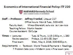
Economics of International Financial Policy: ITF 220 Staff -- Professor: Jeffrey Frankel , Littauer 217 Office hours: Mon.& Tues., 3:00-4:00. Faculty Asst.: Minoo Ghoreishi, Belfer 505 (617) 384-7329 Teaching Fellow: Martin Kessler Course Assistant: Ed Cuipa Times – Lectures: Tues. & Thurs., 1:15-2:30 p.m., L 280 Review session: Fridays, 11:45-1:00, Starr Final exam: Wed., May 4, 2016, 3:00-6:00 p.m.Requirements -- Textbook: World Trade & Payments + Readings. 7 Problem Sets (20%) + Midterm (30%) + Final exam (50%).

Professor Jeffrey Frankel, Kennedy School, Harvard University Big topics covered in the courseI) ELASTICITIES & THE TRADE BALANCEII) THE KEYNESIAN MODEL OF INCOME MONEY AND THE BALANCE OF PAYMENTSIV) GLOBALIZATION OF FINANCIAL MARKETSV) FISCAL & MONETARY POLICY UNDER INTERNATIONAL CAPITAL MOBILITYVI) INTERDEPENDENCE AND COORDINATION VII) SUPPLY, INFLATION & MONETARY UNION VIII) EXPECTATIONS & DETERMINATION OF THE EXCHANGE RATE

Lecture 1: Balance of Payments Accounting Lecture 2: Supply & demand for foreign exchange; export and import elasticities Lecture 3: Empirical effects of devaluation on the trade balanceTOPIC I: ELASTICITIES & THE TRADE BALANCE

Professor Jeffrey Frankel, Kennedy School, Harvard University Lecture 1:Balance of payments accountingDefinition: The balance of payments is the year’s record of economic transactions between domestic and foreign residents. The rules:If you have to pay a foreign resident, normally in exchange for something that you bring into the country, then the something counts as a debit.If a foreign resident has to pay you for something, then the something counts as a credit.

NOW CALLED “FINANCIAL ACCOUNT” “Primary income,” mainly investment income ≡ “secondary income”

Examples of a debit on the current account: You, an American, buy DVDs from India=> import appears as debit on US merchandise account.You import services (electronically) of an Indian software firm => debit appears on US services account (“overseas outsourcing”).You buy the services, instead, from a subsidiary that the Indian software firm set up last year in the US. This is not an international transaction, and so does not appear in the accounts.But assume the subsidiary then sends profits back to India => US reports payments of investment income. It is as if the US is paying for the services of Indian capital. Employees of the subsidiary in the US (or any other US resident entities) send money to relatives back in India => US reports paying unilateral transfers . API-120 - Prof.J.Frankel, Harvard University

Examples of debits on the financial account(previously “capital account”), long-termInstead of buying DVDs from India, you buy the company in India that makes them. => acquisition of assets (debit) under Foreign Direct Investment (FDI). Instead of buying the entire company in India, you buy some stock in it => acquisition of portfolio investments (equities). Instead of buying stock in the company, you lend it money for 2 years => acquisition of portfolio investments (bonds or bank loans). API-120 - Prof.J.Frankel, Harvard University

Examples of debits on the financial account, short term:You lend to the Indian company in the form of 30-day commercial paper or trade credit => acquisition of short term assets (Debit: You have “imported” a claim against India.)You lend to the Indian company in the form of cash dollars, which it doesn’t have to pay back for 30 days => acquisition of short term assets .You are the Central Bank, and you buy securities of the Indian company (an improbable example for the Fed – but some central banks now diversify international investments) => increase in US official reserve assets. API-120 - Prof.J.Frankel, Harvard University

The rules, continuedEach transaction is recorded twice: an import of a good or security has to be paid for.E.g., when an importer pays cash dollars, the import on the merchandise account is offset under short-term capital: the exporter in the other country has, at least for the moment, increased holdings of US assets, which counts just like any other portfolio investment in US assets.At the end of each quarter, credits & debits are added up within each line-item;and line-items are cumulated from the top to compute measures of external balance. API-120 - Prof.J.Frankel, Harvard University

Professor Jeffrey Frankel, Kennedy School, Harvard University Goods &ServicesBalance US trade deficit in goods is partially offset by a surplus in services.CurrentAccountMeasures of US external balance, 2006-2015 PER QUARTER US surplus in investment income is partially offset by outward transfers .

Some balance of payments identitiesCA ≡ Rate of increase in net international investment position.CA-surplus country (Japan) accumulates claims against foreigners;CA-deficit country (US) borrows from foreigners.CA + KA + ORT ≡ 0 .BoP ≡ CA + KA .=> BoP ≡ -ORT ≡ excess supply of FX coming from private sector, (i.e., all credits from exports of goods, services, assets… minus all debits)which central bank absorbs into reserves, if it intervenes in FX market.A BoP surplus country adds to its FX reserves A BoP deficit country either runs down its FX reserves or, is lucky enough for foreign central banks to finance the deficit, if its currency is an international reserve asset (US $) .A floating country does not intervene in the FX market=> BP ≡ 0;Exchange rate E adjusts to clear FX supply & demand in private market

Professor Jeffrey Frankel, Kennedy School, Harvard University End of Lecture 1:Balance of Payments Accounting

Professor Jeffrey Frankel, Kennedy School, Harvard University Lecture 2: The Elasticities Approach to the Trade BalanceQuestion: Under what circumstances does devaluation improve the trade balance (TB), and how much?Model: Elasticities ApproachKey equation: Marshall-Lerner Condition

Supply & demand for foreign exchange D SProfessor Jeffrey Frankel, Kennedy School, Harvard University E ≡price offoreignexchangein $/₤Quantity of foreign exchange, ₤FX supply arises from exports,capital inflows… FX demand arises from imports, capital outflows…

Professor Jeffrey Frankel, Kennedy School, Harvard University Depreciation (increase in price of foreign currency)Deficit (excess demand for foreign currency) Assume demand for forex shifts out e.g., to due to increase in demand to buy foreign goods or assets

Professor Jeffrey Frankel, Kennedy School, Harvard University The Elasticities Approach to the Trade Balancederives the supply of foreign exchange from export earnings, and derives the demand for foreign exchange from import spending.Capital flows are not considered (until later), so no supply of, or demand for, FX comes from international borrowing or lending.

How the Exchange Rate, E, Influences BoPASSUMPTIONS : Supply of FX determined by EXPORT earnings Demand for FX determined by IMPORT spending No capital flows or transfers => BoP = TB 2) PCP: Price in terms of producer’s currency; Supply elasticity = ∞ . => Domestic firms set .   & Foreign firms set .   3) Complete exchange rate passthrough: Price of X in foreign currency = / E   Price of Imports in domestic currency = E   4) Demand is a decreasing function of price in consumer’s currency => X = X D ( / E ) .   => M = M D ( E ) .   => Net supply of FX = TB expressed in foreign currency ≡ TB* = ( /E ) X D ( / E ) - ( ) M D ( E ) .  

How the TB is affected by the exchange rate (continued)EXPERIMENT : E↑ THREE EFFECTS (1) IMD( ) falls. TB* = (/E) XD( /E) - () IMD(E ) . TRADE BALANCE EXPRESSED IN FOREIGN CURRENCY EFFECT ON TB* + + - (2) X D ( ) rises. (3) Price of X in terms of foreign currency falls . Net effect on TB* is determined by Marshall-Lerner condition. Add one more assumption: Before the devaluation, TB*= 0, so export earnings cancel out import spending, Then devaluation improves the TB iff : ε X + ε M > 1 .

Example (i) to illustrate Marshall-Lerner conditionfor TB* = (/E) XD(/E) - ( ) IMD(E)   If εx =1, then E ↑ leaves export revenue unchanged. Because effects (2) and (3) cancel out. In that case, so long as εM > 0, Marshall-Lerner condition is satisfied: Import spending falls -- effect (1) -- => TB* improves.Professor Jeffrey Frankel, Kennedy School, Harvard University

Example (ii) to illustrate Marshall-Lerner conditionfor TB* = (/E) XD(/E) - () IMD(E ) .  If εx = 0, then E ↑ cuts export revenue in proportion because of valuation effect (3). In that case, is εM > 1 necessary to improve TB* ? Yes, because of Marshall-Lerner condition -- fall in import spending then outweighs fall in export revenue: effect (1) > effect (2) -- provided initial X revenue > import spending. But if initial TB*<0, elasticities need not be as high.

How the TB is affected by the exchange rate (continued)EXPERIMENT : E↑ THREE EFFECTS (2) IMD( ) falls. TB = () XD(/E) - (E ) IMD(E ) . TRADE BALANCE EXPRESSED IN DOMESTIC CURRENCY EFFECT ON TB + + - (1) X D ( ) rises. (3) Price of IMports in terms of domestic currency rises. Net effect on TB is determined by the same Marshall-Lerner condition. Again, assume that initially TB=0. Then devaluation improves the TB iff : ε X + ε M > 1 .

Example (iii) to illustrate Marshall-Lerner conditionfor TB* = () XD(/E) - (E ) IMD(E)   If εM =1, then E ↑ leaves import spending unchanged. Because effects (2) and (3) cancel out. In that case, so long as εX > 0, Marshall-Lerner condition is satisfied: Export revenue rises falls -- effect (1) -- => TB improves. Professor Jeffrey Frankel, Kennedy School, Harvard University

Professor Jeffrey Frankel, Kennedy School, Harvard University End ofLecture 2:Elasticities Approach to the Trade Balance

Lecture 3: Empirical effects of the exchange rate on the trade balance Elasticity Pessimism:Countries often fear their elasticities are too low for M-L condition. Econometric estimation of elasticities • What is OLS regression? • Typical estimates The J-curve • With fast pass-through to import prices • With slow pass-through to import prices . An example when it worked: Poland after 2008 . Income as another determinant of the trade balance.

Poland’s exchange rate rose 35% in the 2008-09 global crisis. Zloty / € Source: Cezary WójcikDepreciation boosted net exports => Poland avoided recession Exchange rate

Poland’s trade balance improved sharply in 2009while its European trading partners all went into recession.Source: National Bank of Poland From FocusEconomics 2014 Trade balance in billions of eurosContribution of Net X in 2009: 3.1% of GDP > Total GDP growth: 1.7%

Professor Jeffrey Frankel, Kennedy School, Harvard University How can we estimate sensitivity of export demand to exchange rate?OLS regression . . . . . . . . . . . . . . . X ≡ Exports demanded EP*/P ≡ Price of foreign goods relative to domestic goods

Common econometric findingEstimated trade elasticities with respect to relative prices often ≈ 1, after a few years have been allowed to pass.=> Marshall-Lerner condition holds in the medium run.Some face a higher elasticity of demand for their exports:small countries, andproducers of agricultural & mineral commodities or other commodities that are close substitutes for competitors’ exports.

Common empirical observation:After a devaluation, trade balance gets worse before it gets better. Explanation:Even if devaluation is instantly passed throughto higher import prices,buyers react with a lag.Also, in practice,it often takes time before the devaluation is passed through to import prices.

Another historical example: Mexican & Korean trade balances improvedafter 1994 & 1997 devaluations, respectively

Imports & exports depend on both income and prices: ITF220 - Prof. J. Frankel, Harvard UniversityM = MD [(E ) , Y] X = XD [(/E ), Y*] But in crises like Mexico 1994 or Korea 1997, much of the “improvement” in the trade balance is due to a fall in income Y, which reduces imports.or, more simply:  X = XD (E, Y*) M = MD ( E, Y) .

Estimated price elasticities (LR) satisfy the Marshall-Lerner Condition.Estimated income elasticities are mostly between 1.0 - 2.0. Econometric estimates of elasticities.

Professor Jeffrey Frankel, Kennedy School, Harvard University End ofLecture 3:Empirical Effects of Devaluation on the Trade Balance