PDF-Incorporating "sinuous connectivity" into stochastic models of crustal

Author : yoshiko-marsland | Published Date : 2016-08-02

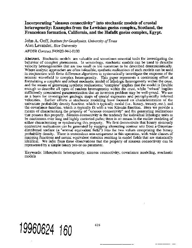
heterogeneity Examples from the Lewisian gneiss complex Scotland the Francsican formation California and the Hafafit gneiss complex Egypt John A Goff Institute for

Presentation Embed Code

<iframe width="560" height="315" src="https://www.docslides.com/embed/429842" frameborder="0" allowfullscreen></iframe>

Download Presentation

Download Presentation The PPT/PDF document "Incorporating "sinuous connectivity" int..." is the property of its rightful owner. Permission is granted to download and print the materials on this website for personal, non-commercial use only, and to display it on your personal computer provided you do not modify the materials and that you retain all copyright notices contained in the materials. By downloading content from our website, you accept the terms of this agreement.

Incorporating "sinuous connectivity" into stochastic models of crustal: Transcript

Download Document

Here is the link to download the presentation.
"Incorporating "sinuous connectivity" into stochastic models of crustal"The content belongs to its owner. You may download and print it for personal use, without modification, and keep all copyright notices. By downloading, you agree to these terms.