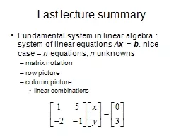
Last lecture summary - PowerPoint Presentation

Slide1

Last lecture summarySlide2

identity vs. similarity

homology vs. similarity

gap penalty

affine gap penalty

gap penalty high

fewer gaps, if investigating related sequences

low

more gaps, larger gaps, distantly related sequencesSlide3

BLOSUM

blocks

focuse

on substitution patterns only

in blocks

BLOSUM62 – 62, what does it mean?

BLOSUM vs. PAM

BLOSUM matrices are based on observed

alignments

BLOSUM numbering system goes in reversing order as the PAM numbering

systemSlide4

Selecting an Appropriate Matrix

Matrix

Best use

Similarity

(%)

Pam40Short highly similar alignments70-90PAM160Detecting members of a protein family50-60PAM250Longer alingments of more divergent sequences~30BLOSUM90Short highly similar alignments70-90BLOSUM80Detecting members of a protein family50-60BLOSUM62Most effective in finding all potential similarities30-40BLOSUM30Longer alingments of more divergent sequences<30

Similarity column gives range of similarities that the matrix is able to best detect.Slide5

Dynamic programming (DP)

Recursive approach, sequential dependency.

4

th

piece can be solved using solution of the 3

rd piece, the 3rd piece can be solved by using solution of the 2nd piece and so on…Slide6

Sequence B

Sequence A

Best previous alignment

New best alignment = previous best + local best

...

...

...

...

If

you already have the optimal solution to:

X…Y

A…B

then you know the

next

pair of characters will either be

:

X…Y

Z

or

X…Y

-

or

X…Y

Z

A…B

C

A…B

C

A…B

-

You

can extend the match by determining which

of these

has the highest score.Slide7

New stuffSlide8

Dot plot

Graphical method that allows the comparison of two biological sequences and identify regions of close similarity between them.

Also used for finding direct or inverted repeats in sequences.

Or for prediction regions in RNA that are self-complementary and therefore have potential to form secondary structures.Slide9
Slide10

Self-similarity dot plot I

The DNA sequence EU127468.1 compared against itself.

Introduction to dot-plots, Jan Schulz

http://www.code10.info/index.php?option=com_content&view=article&id=64:inroduction-to-dot-plots&catid=52:cat_coding_algorithms_dot-plots&Itemid=76Slide11

runs of

matched

residues

gap

background

noiseSlide12

Self-similarity dot plot II

Introduction to dot-plots, Jan Schulz

http://www.code10.info/index.php?option=com_content&view=article&id=64:inroduction-to-dot-plots&catid=52:cat_coding_algorithms_dot-plots&Itemid=76

The DNA sequence EU127468.1 compared against itself.

Window size = 16.

Linear color mappingSlide13

Improving dot plot

Sliding window – window size (lets say 11)

Stringency (lets say 7) – a dot is printed only if 7 out of the next 11 positions in the sequence are identical

Color mapping

Scoring matrices can be used to assign a score to each substitution. These numbers then can be converted to gray/color.Slide14

Interpretation of dot plot I

Plot two homologous sequences of interest. If they

are

similar – diagonal line will occur (

matches

).frame shifts mutations gaps in diagonal insertions shift of main diagonaldeletions shift of main diagonalhttp://ugene.unipro.ru/documentation/manual/plugins/dotplot/interpret_a_dotplot.htmlSlide15

Interpretation of dot plot II

Identify repeat regions (

direct repeats

,

inverted repeats

) – lines parallel to the diagonal line in self-similarity plotMicrosattelites and minisattelites (these are also called low-complexity regions) can be identified as “squares”.Palindromatic sequences are shown as lines perpendicular to the main diagonal.Plaindromatic sequence: V ELIPSE SPI LEVBioinformatics explained: Dot plots, http://www.clcbio.com/index.php?id=1330&manual=BE_Dot_plots.htmlSlide16

Repeats in dot plot

from the book Bioinformatics, David. M. Mount,

direct repeats

minisattelites

inverted repeats

self-similarity dot plot of NA sequence ofhuman LDL receptor

window 23, stringency 7Slide17

Interpretation of dot plot – summary

http://www.code10.info/index.php?option=com_content&view=article&id=64:inroduction-to-dot-plots&catid=52:cat_coding_algorithms_dot-plots&Itemid=76 Slide18

Dot plot of the human genome

A. M. Campbell, L. J. Heyer, Discovering genomics, proteomics and bioinformaticsSlide19

Dot plot rules

Larger windows size is used for DNA sequences because the number of random matches is much greater due to the presence of only four characters in the alphabet.

A typical window size for DNA is 15, with stringency 10. For proteins the matrix has not to be filtered at all, or windows

2 or 3

with stringency 2 can be used.

If two proteins are expected to be related but to have long regions of dissimilar sequence with only a small proportion of identities, such as similar active sites, a large window, e.g., 20, and small stringency, e.g., 5, should be useful for seeing any similarity.Slide20

Dot plot advantages/disadvantages

Advantages

:

All possible matches of residues between two sequences are found. It’s just up to you to choose the most significant ones.

Readily reveals the presence of

insertions/deletions and direct and inverted repeats that are more difficult to find by the other, more automated methods.Disadvantages:Most dot matrix computer programs do not show an actual alignment. Does not return a score to indicate how ‘optimal’ a given alignment is (no statistical significance that could be tested).Slide21

Homology vs. similarity again

Just a reminder of the important concept in sequence analysis –

homology

. It is a conclusion about a common ancestral relationship drawn from sequence similarity.

Sequence

similarity is a direct result of observation from the sequence alignment. It can be quantified using percentages, but homology can not!It is important to understand this difference between homology and similarity.If the similarity is high enough, a common evolutionary relationship can be inferred.Slide22

Limits of

the

alignment detection

However, what is enough? What are the detection limits of pairwise alignments? How many mutations can occur before the differences make two sequences unrecognizable?

Intuitively, at some point are two homologous sequences too divergent for their alignment to be recognized as significant.

The best way to determine detection limits of pairwise alignment is to use statistical hypothesis testing. See later.Slide23

Twilight zone

However, the level one can infer homologous relationship depends on type of sequence (proteins, NA) and on the length of the alignment.

Unrelated sequences of DNA have at least 25% chance to be identical. For proteins it is 5%. If gaps are allowed, this percentage can increase up to 10-20%.

The shorter the sequence, the higher the chance that some alignment is attributable to random chance.

This suggest that shorter sequences require higher cuttof for inferring homology than longer sequences.Slide24

Essential bioinformatics, XiongSlide25

Statistical significance

Key question

– Constitutes a given alignment evidence for homology? Or did it occur just by chance?

The statistical significance of the alignment (i.e. its score) can be tested by statistical hypotheses testing.Slide26

Significance of global alignment I

We align two proteins: human beta globin and myoglobin. We obtain score

S

.

And we want to know if such

a score is significant or if it appeared just by a chance. How to proceed?State H0 two sequences are not related, score S represents a chance occurrenceState HaChoose a significance level What else do we have to know?statistics of distribution. i.e. what?sample mean, sample standard deviation Slide27

Significance of global alignment

II

How

to

determine the parameters of distribution?

Compare S to scores of beta globin/myoglobin relative to a large number of sequences of non-homologous proteinsCompare with a set of randomly generated sequences.Keep the beta globin and randomly scramble the sequence of myoglobin.Performing any of the previous, we obtain the sample mean and sample standard deviation.A Z-score can be calculated. How? Slide28

Significance

of global alignment

II

I

For

normal distribution, if Z=3 99.74% of the scores are within how many stdev of the mean?threeAnd the fraction of scores greater is?We can expect to see this particular high score by chance about 1 time in 750 (1/750 ≈ 0.13%)0.26% is represented as confidence level .In hypotheses testing, commonly used is . Slide29
Slide30

Significance of global alignment

IV

The problem with this approach is if the distribution is not Gaussian.

Then the estimated significance level will be wrong.

Bad news – distribution of global alignments is generally not Gaussian and no theory exists.

Another consideration – problem of multiple comparisonsIf we compare query sequence to 1 million sequences in database, we have a million chances to find a high scoring match. In such case it is appropriate to adjust to more stringent level.Bonferroni correction –  Slide31

Significance of

local alignment

In contrast to global alignment there is a thorough understanding of the distribution of scores.

Key role play

Extreme value distributions

(EVD)Generate N data sets from the same distribution, create a new data set that includes the maximum/minimum values from these N data sets, the resulting data set can only be described by one of the three distributionsGumbel, Fréchet, Weibullapplicationsextreme floods, large wildfireslarge insurance lossessize of freak wavessequence alignment Slide32

Gumbel distribution

… location parameter

… scale parameter

wikipedia.orgSlide33

Statistical distribution of alignments

local alignment

analytical theory

gapless – Gumbel, parameters can be evaluated analytically

gapped – Gumbel,

parameters must be obtained from simulations, no analytical formulasglobal alignmentno thorough theory, however empirical simulations show that the distribution is also Gumbel