Several slides from Larry Zitnick and Steve Seitz Why do we perceive depth What do humans use as depth cues Convergence When watching an object close to us our eyes point slightly inward This difference in the direction of the eyes is called convergence This depth cue is effective only ID: 915156
Download Presentation The PPT/PDF document "Stereo CSE 455 Ali Farhadi" is the property of its rightful owner. Permission is granted to download and print the materials on this web site for personal, non-commercial use only, and to display it on your personal computer provided you do not modify the materials and that you retain all copyright notices contained in the materials. By downloading content from our website, you accept the terms of this agreement.
Slide1
Stereo
CSE 455
Ali Farhadi
Several slides from Larry
Zitnick
and Steve Seitz
Slide2Slide3Why do we perceive depth?
Slide4What do humans use as depth cues?
Convergence
When watching an object close to us, our eyes point slightly inward. This difference in the direction of the eyes is called convergence. This depth cue is effective only on short distances (less than 10 meters).
Marko
Teittinen
http://www.hitl.washington.edu/scivw/EVE/III.A.1.c.DepthCues.html
Motion
Focus
Binocular Parallax
As our eyes see the world from slightly different locations, the images sensed by the eyes are slightly different. This difference in the sensed images is called binocular parallax. Human visual system is very sensitive to these differences, and binocular parallax is the most important depth cue for medium viewing distances. The sense of depth can be achieved using binocular parallax even if all other depth cues are removed.
Monocular Movement Parallax
If we close one of our eyes, we can perceive depth by moving our head. This happens because human visual system can extract depth information in two similar images sensed after each other, in the same way it can combine two images from different eyes.
Accommodation
Accommodation is the tension of the muscle that changes the focal length of the lens of eye. Thus it brings into focus objects at different distances. This depth cue is quite weak, and it is effective only at short viewing distances (less than 2 meters) and with other cues.
Slide5What do humans use as depth cues?
Shades and Shadows
When we know the location of a light source and see objects casting shadows on other objects, we learn that the object shadowing the other is closer to the light source. As most illumination comes downward we tend to resolve ambiguities using this information. The three dimensional looking computer user interfaces are a nice example on this. Also, bright objects seem to be closer to the observer than dark ones.
Marko
Teittinen
http://www.hitl.washington.edu/scivw/EVE/III.A.1.c.DepthCues.html
Image cues
Retinal Image Size
When the real size of the object is known, our brain compares the sensed size of the object to this real size, and thus acquires information about the distance of the object.
Linear Perspective
When looking down a straight level road we see the parallel sides of the road meet in the horizon. This effect is often visible in photos and it is an important depth cue. It is called linear perspective.
Texture Gradient The closer we are to an object the more detail we can see of its surface texture. So objects with smooth textures are usually interpreted being farther away. This is especially true if the surface texture spans all the distance from near to far. Overlapping When objects block each other out of our sight, we know that the object that blocks the other one is closer to us. The object whose outline pattern looks more continuous is felt to lie closer. Aerial HazeThe mountains in the horizon look always slightly bluish or hazy. The reason for this are small water and dust particles in the air between the eye and the mountains. The farther the mountains, the hazier they look.
Jonathan Chiu
Slide6Slide7Amount of horizontal movement is …
…inversely proportional to the distance from the camera
Slide8Depth from StereoGoal: recover depth by finding image coordinate x’ that corresponds to x
f
x
x’
Baseline
B
z
C
C’
X
f
X
x
x'
Slide9Depth from disparity
f
x’
Baseline
B
z
O
O’
X
f
Disparity is inversely proportional to
depth.
x
Slide10Depth from Stereo
Goal: recover depth by finding image coordinate x’ that corresponds to x
Sub-Problems
Calibration: How do we recover the relation of the cameras (if not already known)?
Correspondence: How do we search for the matching point x’?
X
x
x'
Slide11Correspondence Problem
We have two images taken from cameras with different intrinsic and extrinsic parameters
How do we match a point in the first image to a point in the second? How can we constrain our search?
x
?
Slide12Potential
matches for
x
have to lie on the corresponding
line l’.
Potential matches for x’ have to lie on the corresponding line l.
Key idea:
Epipolar
constraint
x
x’
X
x’
X
x’
X
Slide13Epipolar
Plane
– plane containing baseline (1D family)
Epipoles
= intersections of baseline with image planes
= projections of the other camera center
Baseline
– line connecting the two camera centers
Epipolar
geometry: notation
X
x
x’
Slide14Epipolar
Lines
- intersections of
epipolar
plane with image
planes (always come in corresponding pairs)
Epipolar
geometry: notation
X
x
x’
Epipolar
Plane
– plane containing baseline (1D family)
Epipoles
= intersections of baseline with image planes
= projections of the other camera center
Baseline
– line connecting the two camera centers
Slide15Example: Converging cameras
Slide16Example: Motion parallel to image plane
Slide17Example: Forward motion
What would the
epipolar
lines look like if the camera moves directly forward?
Slide18Example: Motion perpendicular to image plane
Slide19Example: Motion perpendicular to image plane
Points move along lines radiating from the
epipole
: “focus of expansion”
Epipole is the principal point
Slide20e
e’
Example: Forward motion
Epipole
has same coordinates in both images.
Points move along lines radiating from
“Focus of expansion”
Slide21Epipolar constraint
If we observe a point
x
in one image, where can the corresponding point
x’ be in the other image?
x
x’
X
Slide22Potential matches for
x
have to lie on the corresponding
epipolar line l
’. Potential matches for x’ have to lie on the corresponding epipolar
line l.
Epipolar constraint
x
x’
X
x’
X
x’
X
Slide23Epipolar constraint example
Slide24X
x
x’
Epipolar constraint: Calibrated case
Assume that the intrinsic and extrinsic parameters of the cameras are known
We can multiply the projection matrix of each camera (and the image points) by the inverse of the calibration matrix to get
normalized
image coordinates
We can also set the global coordinate system to the coordinate system of the first camera. Then the projection matrices of the two cameras can be written as
[I | 0]
and
[R | t]
Slide25X
x
x
’ =
Rx+t
Epipolar constraint: Calibrated case
R
t
The vectors
Rx
,
t
, and
x
’
are coplanar
=
(
x,
1)
T
Slide26Essential Matrix
(Longuet-Higgins, 1981)
Epipolar constraint: Calibrated case
X
x
x’
The vectors
Rx
,
t
, and
x
’
are coplanar
Slide27X
x
x’
Epipolar constraint: Calibrated case
E x
is the
epipolar
line associated with
x
(
l
'
= E x)E
Tx' is the epipolar line associated with x' (l = ETx')E e = 0 and ETe' = 0E is singular (rank two)E has five degrees of freedom
Slide28Epipolar constraint: Uncalibrated case
The calibration matrices
K
and
K’ of the two cameras are unknownWe can write the epipolar constraint in terms of
unknown normalized coordinates:
X
x
x’
Slide29Epipolar constraint: Uncalibrated case
X
x
x’
Fundamental Matrix
(Faugeras and Luong, 1992)
Slide30Epipolar constraint: Uncalibrated case
F
x
is the
epipolar line associated with x (l' = F x)
FTx' is the epipolar line associated with x' (l' =
F
T
x
')F e = 0 and FTe
' = 0F
is singular (rank two)F has seven degrees of freedom
X
xx’
Slide31The eight-point algorithm
Minimize:
under the constraint
||
F
||
2
=1
Smallest eigenvalue of A
T
A
A
Slide32The eight-point algorithm
Meaning of error
sum of squared
algebraic
distances between points x’i and
epipolar lines F xi (or points xi and epipolar lines FT
x’i) Nonlinear approach: minimize sum of squared geometric distances
Slide33Problem with eight-point algorithm
Slide34Problem with eight-point algorithm
Poor numerical conditioning
Can be fixed by rescaling the data
Slide35The normalized eight-point algorithm
Center the image data at the origin, and scale it so the mean squared distance between the origin and the data points is 2 pixels
Use the eight-point algorithm to compute
F
from the normalized pointsEnforce the rank-2 constraint (for example, take SVD of F and throw out the smallest singular value)
Transform fundamental matrix back to original units: if T and T’ are the normalizing transformations in the two images, then the fundamental matrix in original coordinates is T’T
F T(Hartley, 1995)
Slide36Comparison of estimation algorithms
8-point
Normalized 8-point
Nonlinear least squares
Av. Dist. 1
2.33 pixels
0.92 pixel
0.86 pixel
Av. Dist. 2
2.18 pixels
0.85 pixel
0.80 pixel
Slide37Moving on to stereo… Fuse a calibrated binocular stereo pair to produce a depth image
image 1
image 2
Dense depth map
Many of these slides adapted from Steve Seitz and Lana Lazebnik
Slide38Depth from disparity
f
x’
Baseline
B
z
O
O’
X
f
Disparity is inversely proportional to
depth.
x
Slide39Basic stereo matching algorithm
If necessary, rectify the two stereo images to transform
epipolar
lines into
scanlines
For each pixel x in the first image
Find corresponding
epipolar
scanline
in the right image
Search the scanline and pick the best match x’
Compute disparity x-x’ and set depth(x) = fB/(x-x’)
Slide40Basic stereo matching algorithm
For each pixel in the first image
Find corresponding
epipolar
line in the right image
Search along
epipolar
line and pick the best match
Triangulate the matches to get depth information
Simplest case:
epipolar
lines are
scanlinesWhen does this happen?
Slide41Simplest Case: Parallel images
Epipolar constraint:
R = I t
= (
T
, 0, 0)
The y-coordinates of corresponding points are the
same
t
x
x’
Slide42Stereo image rectification
Slide43Stereo image rectification
Reproject
image planes onto a common plane parallel to the line between camera centers
Pixel motion is horizontal after this transformation
Two
homographies
(3x3 transform), one for each input image
reprojection
C. Loop and Z. Zhang.
Computing Rectifying
Homographies
for Stereo Vision
. IEEE Conf. Computer Vision and Pattern Recognition, 1999
.
Slide44Example
Unrectified
Rectified
Slide45Matching cost
disparity
Left
Right
scanline
Correspondence search
Slide a window along the right scanline and compare contents of that window with the reference window in the left image
Matching cost: SSD or normalized correlation
Slide46Left
Right
scanline
Correspondence search
SSD
Slide47Left
Right
scanline
Correspondence search
Norm. corr
Slide48Effect of window size
W = 3
W = 20
Smaller window
+ More detail
More noise
Larger window
+ Smoother disparity maps
Less detail
Fails near boundaries
Slide49Failures of correspondence search
Textureless surfaces
Occlusions, repetition
Non-Lambertian surfaces, specularities
Slide50Results with window search
Window-based matching
Ground truth
Data
Slide51How can we improve window-based matching?
So far, matches are independent for each point
What constraints or priors can we add?
Slide52Stereo constraints/priors
Uniqueness
For any point in one image, there should be at most one matching point in the other image
Slide53Stereo constraints/priors
Uniqueness
For any point in one image, there should be at most one matching point in the other image
Ordering
Corresponding points should be in the same order in both views
Slide54Stereo constraints/priors
Uniqueness
For any point in one image, there should be at most one matching point in the other image
Ordering
Corresponding points should be in the same order in both views
Ordering constraint doesn’t hold
Slide55Priors and constraints
Uniqueness
For any point in one image, there should be at most one matching point in the other image
Ordering
Corresponding points should be in the same order in both viewsSmoothnessWe expect disparity values to change slowly (for the most part)
Slide56Stereo as energy minimization
What defines a good stereo correspondence?
Match quality
Want each pixel to find a good match in the other image
SmoothnessIf two pixels are adjacent, they should (usually) move about the same amount
Slide57Stereo as energy minimizationBetter objective function
{
{
match cost
smoothness cost
Want each pixel to find a good match in the other image
Adjacent pixels should (usually) move about the same amount
Slide58Stereo as energy minimization
match cost:
smoothness cost:
4-connected neighborhood
8-connected neighborhood
: set of neighboring pixels
SSD distance between windows
I
(
x
,
y
) and
J
(
x
,
y
+
d
(
x
,
y
))
=
Slide59Smoothness cost
“
Potts model
”
L
1
distance
Slide60Dynamic programmingCan minimize this independently per scanline using dynamic programming (DP)
: minimum cost of solution such that
d
(
x
,
y
) =
d
Slide61Energy minimization via graph cuts
Labels
(disparities)
d
1
d
2
d
3
edge weight
edge weight
Slide62d
1
d
2
d
3
Graph Cut
Delete enough edges so that
each pixel is connected to exactly one label node
Cost of a cut: sum of deleted edge weights
Finding min cost cut equivalent to finding global minimum of energy function
Energy minimization via graph cuts
Slide63Stereo as energy minimization
I
(
x
,
y
)
J
(
x
,
y
)
y = 141
C
(
x
,
y
,
d
); the
disparity space image
(DSI)
x
d
Slide64Stereo as energy minimization
y = 141
x
d
Simple pixel / window matching: choose the minimum of each column in the DSI independently:
Slide65Matching windows
Similarity Measure
Formula
Sum of Absolute Differences (SAD)
Sum of Squared Differences (SSD)
Zero-mean SAD
Locally scaled SAD
Normalized Cross Correlation (NCC)
http://siddhantahuja.wordpress.com/category/stereo-vision/
SAD
SSD
NCC
Ground truth
Slide66Before & After
Graph cuts
Ground truth
For the latest and greatest:
http://www.middlebury.edu/stereo/
Y. Boykov, O. Veksler, and R. Zabih,
Fast Approximate Energy Minimization via Graph Cuts
, PAMI 2001
Before
Slide67Real-time stereo
Used for robot navigation (and other tasks)
Several software-based real-time stereo techniques have been developed (most based on simple discrete search)
Nomad robot
searches for meteorites in Antartica
http://www.frc.ri.cmu.edu/projects/meteorobot/index.html
Slide68Why does stereo fail?
Fronto
-Parallel Surfaces: Depth is constant within the region of local support
Slide69Why does stereo fail?Monotonic Ordering - Points along an epipolar scanline appear in the same order in both stereo images
Occlusion – All points are visible in each image
Slide70Why does stereo fail?
Image Brightness Constancy: Assuming
Lambertian
surfaces, the brightness of corresponding
points in stereo images are the same.
Slide71Why does stereo fail?
Match Uniqueness: For every point in one stereo image, there is at most one corresponding point in the other image.
Slide72Camera calibration errors
Poor image resolution
Occlusions
Violations of brightness constancy (specular reflections)
Large motions
Low-contrast image regions
Stereo reconstruction pipelineStepsCalibrate camerasRectify imagesCompute disparityEstimate depth
What will cause errors?
Slide73width of
a pixel
Choosing the stereo baseline
What
’
s the optimal baseline?
Too small: large depth error
Too large: difficult search problem
Large Baseline
Small Baseline
all of these
points project
to the same
pair of pixels
Slide74Multi-view stereo ?
Slide75The third view can be used for verification
Beyond two-view stereo
Slide76Using more than two images
Multi-View Stereo for Community Photo Collections
M. Goesele, N. Snavely, B. Curless, H. Hoppe, S. Seitz
Proceedings of
ICCV 2007
,