/
Chapter 2:  Business Efficiency Chapter 2:  Business Efficiency

Chapter 2: Business Efficiency - PowerPoint Presentation

briana-ranney
briana-ranney . @briana-ranney
Follow
374 views
Uploaded On 2018-03-19

Chapter 2: Business Efficiency - PPT Presentation

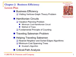
Lesson Plan Business Efficiency Visiting VerticesGraph Theory Problem Hamiltonian Circuits Vacation Planning Problem Minimum CostHamiltonian Circuit Method of Trees Fundamental Principle of Counting ID: 657145

hamiltonian circuit vertex edges circuit hamiltonian edges vertex cost business chapter graph vertices circuits starting order problem tour tasks

Share:

Link:

Embed:

Download Presentation from below link

Download Presentation The PPT/PDF document "Chapter 2: Business Efficiency" is the property of its rightful owner. Permission is granted to download and print the materials on this web site for personal, non-commercial use only, and to display it on your personal computer provided you do not modify the materials and that you retain all copyright notices contained in the materials. By downloading content from our website, you accept the terms of this agreement.


Presentation Transcript

Slide1

Chapter 2: Business EfficiencyLesson Plan

Business EfficiencyVisiting Vertices-Graph Theory Problem Hamiltonian Circuits Vacation Planning ProblemMinimum Cost-Hamiltonian CircuitMethod of TreesFundamental Principle of CountingTraveling Salesman ProblemHelping Traveling SalesmenNearest Neighbor and Sorted Edges AlgorithmsMinimum-Cost Spanning TreesKruskal’s AlgorithmCritical-Path Analysis

1

Mathematical Literacy in Today’s World, 9th ed.

For All Practical Purposes

© 2013 W. H. Freeman and CompanySlide2

Chapter 2: Business EfficiencyBusiness Efficiency

Visiting Vertices In some graph theory problems, it is only necessary to visit specific locations (using the travel routes, or streets available).Problem: Find an efficient route along distinct edges of a graph that visits each vertex only once in a simple circuit. 2 Applications:Salesman visiting particular citiesDelivering mail to drop-off boxesRoute taken by a snowplowPharmaceutical representative visiting doctors Slide3

Hamiltonian CircuitA tour that starts and ends at the same vertex (circuit definition).

Visits each vertex once. (Vertices cannot be reused or revisited.)Circuits can start at any location. Use wiggly edges to show the circuit.3 Starting at vertex A, the tour can be written as ABDGIHFECA, or starting at E, it would be EFHIGDBACE.Chapter 2: Business EfficiencyHamiltonian CircuitA different circuit visiting each vertex once and only once would be CDBIGFEHAC (starting at vertex C).Slide4

Hamiltonian vs. Euler Circuits

SimilaritiesBoth forbid re-use.Hamiltonian do not reuse vertices.Euler do not reuse edges.DifferencesHamiltonian is a circuit of vertices.Euler is a circuit of edges.Euler graphs are easy to spot (connectedness and even valence).Hamiltonian circuits are NOT as easy to determine upon inspection.Some certain family of graphs can be known to have or not have Hamiltonian circuits. 4 Chapter 2: Business EfficiencyHamiltonian Circuit vs. Euler CircuitsHamiltonian circuit – A tour (

shown by wiggly edges) that starts at a vertex of a graph and visits each vertex once and only once, returning to where it started.

Euler circuit – A circuit that traverses each edge

of a graph exactly once and starts and stops at the same point. Slide5

Chapter 2: Business EfficiencyHamiltonian Circuits

Vacation-Planning ProblemHamiltonian circuit concept is used to find the best route that minimizes the total distance traveled to visit friends in different cities. (assume less mileage  less gas  minimizes costs) Road mileage between four cities5 Hamiltonian circuit with weighted edges Edges of the graph are given weights, or in this case mileage or distance between cities. As you travel from vertex to vertex, add the numbers (mileage in this case).Each Hamiltonian circuit will produce a particular sum. Slide6

Chapter 2: Business EfficiencyHamiltonian Circuit

Algorithm – A step-by-step description of how to solve a problem.Minimum-Cost Hamiltonian Circuit A Hamiltonian circuit with the lowest possible sum of the weights of its edges.Algorithm (step-by-step process) for Solving This Problem6 Generate all possible Hamiltonian tours (starting with Chicago).

Add up the distances on the edges of each tour.Choose the tour of minimum distance. Slide7

Chapter 2: Business EfficiencyHamiltonian Circuits

Method of trees for vacation-planning problem7 Method of Trees For the first step of the algorithm, a systematic approach is needed to generate all possible Hamiltonian tours (disregard distances during this step).This method begins by selecting a starting vertex, say Chicago, and making a tree diagram showing the next possible locations.At each stage down, there will be one less choice (3, 2, then 1 choice).In this example, the method of trees generated six different paths, all starting and ending with Chicago. However, only three of these are unique circuits. Slide8

Chapter 2: Business EfficiencyHamiltonian Circuits

8 The three Hamiltonian circuits’ sums of the toursMinimum-Cost Hamiltonian Circuit: Vacation-Planning ExampleMethod of trees used to find all tours (for four cities: three unique paths). On the graph, the unique paths are drawn with wiggly lines.Add up the distances on the edges of each unique tour.

Choose the tour of minimum distance. The smallest sum would give us the minimal distance, which is the minimum cost.Slide9

Chapter 2: Business EfficiencyHamiltonian Circuit

9 Principle of Counting (for Hamiltonian Circuits)For a complete graph of n vertices, there are (n - 1)! possible routes.Since half of these routes are repeats, the result is:Possible unique Hamiltonian circuits are (n - 1)! / 2Complete graph – A graph in which every pair of vertices is joined by an edge.Fundamental Principle of Counting

If there are a ways of choosing one thing,b ways of choosing a second after the first is chosen,

c ways of choosing a third after the second is chosen, and so on…,and z ways of choosing the last item after the earlier choices,then the total number of choice patterns is a × b × c

× … × z.Example: Jack has 9 shirts and 4 pairs of pants. He can wear 9 × 4 = 36 shirt-pant outfits.Slide10

10

Traveling Salesman Problem (TSP)Difficult to solve Hamiltonian circuits when the number of vertices in a complete graph increases (n becomes very large). This problem originated from a salesman determining his trip that minimizes costs (less mileage) as he visits the cities in a sales territory, starting and ending the trip in the same city.There are many applications today: bus schedules, mail drop-offs, telephone booth coin pick-up routes, electric company meter readers, etc.How can the TSP be solved?Computer programs can find the optimal route (not always practical). Heuristic methods can be used to find a “fast” answer, but does not guarantee that it is always the optimal answer.Nearest neighbor algorithmSorted edges algorithmChapter 2: Business EfficiencyTraveling Salesman ProblemSlide11

Chapter 2: Business EfficiencyTraveling Salesman Problem —

Nearest Neighbor11 Nearest neighbor starting at vertex ANearest Neighbor Algorithm (to solve TSP)Starting from the “home” city (or vertex), first visit the nearest city (one with the least mileage from “home”). As you travel from city to city, always choose the next city (vertex) that can be reached quickest (i.e., nearest with the least miles), that has not already been visited.When all other vertices have been visited, the tour returns home.Nearest neighbor starting at vertex B

Hamiltonian Circuit: A-B-C-E-D-A

Hamiltonian Circuit: B-C-A-D-E-BSlide12

Chapter 2: Business EfficiencyTraveling Salesman Problem —

Sorted EdgesSorted Edges Algorithm (to solve TSP)Start by sorting, or arranging, the edges in order of increasing cost (sort smallest to largest mileage between cities).At each stage, select that edge of least cost until all the edges are connected at the end while following these rules:If an edge is added that results in three edges meeting at a vertex, eliminate the longest edge.Always include all vertices in the finished circuit.12 Example using sorted edges Edges selected are DE at 400, BC at 500, AD at 550, and AB at 600 (AC and AE are not chosen because they result in three edges meeting at A). Lastly, CE at 750 is chosen to complete the circuit of 2800 miles.Slide13

Chapter 2: Business EfficiencyMinimum-Cost Spanning Trees

13 Costs (in millions of dollars) of installing Pictaphone service among five citiesMinimum-Cost Spanning TreesAnother graph theory optimization problem that links all the vertices together, in order of increasing costs, to form a “tree.”The cost of the tree is the sum of the weights on the edges.Example: What is the cost to construct a Pictaphone service (telephone service with video image of the callers) among five cities? The diagram shows the cost to build the connection from each vertex to all other vertices (connected graph).Cities are linked in order of increasing costs to make the connection.The cost of redirecting the signal may be small compared to adding another link.Slide14

Chapter 2: Business EfficiencyMinimum-Cost Spanning Trees

14 Kruskal’s Algorithm — Developed by Joseph Kruskal (AT&T research).Goal of minimum-cost spanning tree: Create a tree that links all the vertices together and achieves the lowest cost to create.Add links in order of cheapest cost according to the rules:No circuit is created (no loops).If a circuit (or loop) is created by adding the next largest link, eliminate this largest (most expensive link)—it is not needed.Every vertex must be included in the final tree.Slide15

Chapter 2: Business EfficiencyCritical Path Analysis

An order-requirement digraph, tasks A – E with task times in the circlesCritical Path is BE = 25 + 27 = 52 min.15 Critical Path Analysis Most often, scheduling jobs consists of complicated tasks that cannot be done in a random order.Due to a pre-defined order of tasks, the entire job may not be done any sooner than the longest path of dependent tasks. Order-Requirement Digraph A directed graph (digraph) that shows which tasks precede other tasks among the collection of tasks making up a job.Critical Path The longest path in an order-requirement digraph. The length is measured in terms of summing the task times of the tasks making up the path.