/
Announcements Midterm: Wednesday 7pm-9pm Announcements Midterm: Wednesday 7pm-9pm

Announcements Midterm: Wednesday 7pm-9pm - PowerPoint Presentation

caitlin
caitlin . @caitlin
Follow
342 views
Uploaded On 2022-06-08

Announcements Midterm: Wednesday 7pm-9pm - PPT Presentation

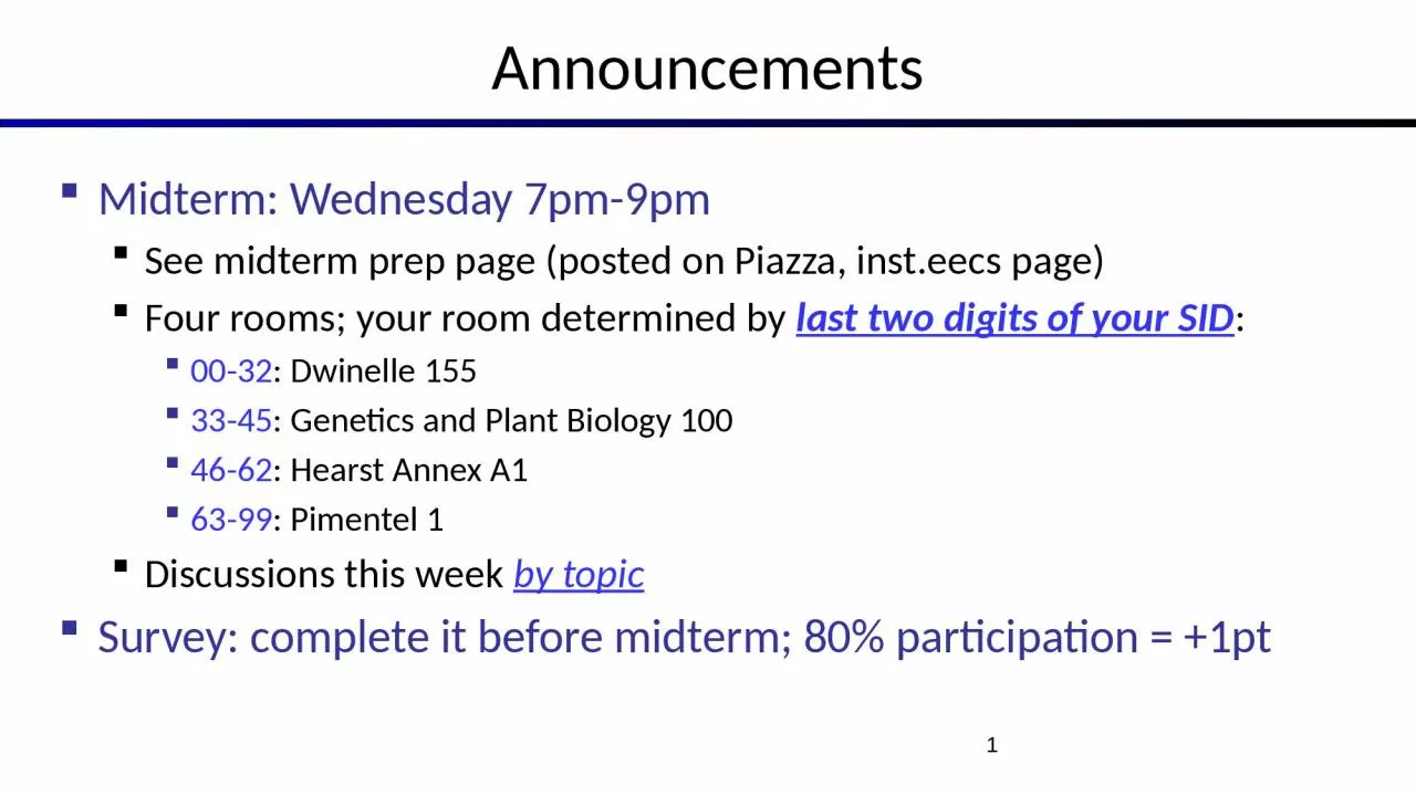
See midterm prep page posted on Piazza insteecs page Four rooms your room determined by last two digits of your SID 0032   Dwinelle 155 3345  Genetics and Plant Biology 100 ID: 915655

false true factors variable true false variable factors factor elimination inference bayes complexity nets joint independent variables sum probability

Share:

Link:

Embed:

Download Presentation from below link

Download Presentation The PPT/PDF document "Announcements Midterm: Wednesday 7pm-9pm" is the property of its rightful owner. Permission is granted to download and print the materials on this web site for personal, non-commercial use only, and to display it on your personal computer provided you do not modify the materials and that you retain all copyright notices contained in the materials. By downloading content from our website, you accept the terms of this agreement.


Presentation Transcript

Slide1

Announcements

Midterm: Wednesday 7pm-9pmSee midterm prep page (posted on Piazza, inst.eecs page)Four rooms; your room determined by last two digits of your SID:00-32: Dwinelle 15533-45: Genetics and Plant Biology 10046-62: Hearst Annex A163-99: Pimentel 1Discussions this week by topicSurvey: complete it before midterm; 80% participation = +1pt

1

Slide2

Bayes net global semantics

Bayes nets encode joint distributions as product of conditional distributions on each variable:P(X1,..,Xn) = i P

(

X

i | Parents(Xi))

Slide3

Conditional independence semantics

Every variable is conditionally independent of its non-descendants given its parentsConditional independence semantics <=> global semantics3

Slide4

Example

JohnCalls independent of Burglary given Alarm?YesJohnCalls independent of MaryCalls given Alarm?YesBurglary independent of Earthquake?YesBurglary independent of Earthquake given Alarm?NO!Given that the alarm has sounded, both burglary and earthquake become more likelyBut if we then learn that a burglary has happened, the alarm is explained away and the probability of earthquake drops back 4

B

urglary

EarthquakeA

larm

J

ohn calls

M

ary calls

V-structure

Slide5

Markov blanket

A variable’s Markov blanket consists of parents, children, children’s other parentsEvery variable is conditionally independent of all other variables given its Markov blanket5

Slide6

CS 188: Artificial Intelligence

Bayes Nets: Exact InferenceInstructor: Sergey Levine and Stuart Russell--- University of California, Berkeley

Slide7

Bayes Nets

Part I: RepresentationPart II: Exact inferenceEnumeration (always exponential complexity)Variable elimination (worst-case exponential complexity, often better)

Inference is NP-hard in general

Part III: Approximate Inference

Later: Learning Bayes nets from data

Slide8

Examples:

Posterior marginal probability

P

(

Q

|

e

1

,..,

e

k

)

E.g., what disease might I have?

Most likely explanation:

argmax

q,r,s

P

(

Q=

q,R

=r,S=s|

e1,..,e

k

)

E.g., what did he say?

Inference

Inference: calculating some useful quantity from a probability model (joint probability distribution)

Slide9

Inference by Enumeration in Bayes Net

Reminder of inference by enumeration:Any probability of interest can be computed by summing entries from the joint distributionEntries from the joint distribution can be obtained from a BN by multiplying the corresponding conditional probabilitiesP(B | j, m) =

α

P

(B, j, m) = α e

,

a

P

(

B

,

e,

a,

j

,

m)

= α e

,a P

(B) P(

e) P(a|

B

,

e

)

P

(

j

|

a

)

P

(

m

|

a)So inference in Bayes nets means computing sums of products of numbers: sounds easy!!Problem: sums of exponentially many products!

B

E

A

M

J

Slide10

Can we do better?

Consider

uwy

+

uwz

+

uxy

+

uxz

+

vwy

+

vwz

+

vxy

+

vxz

16 multiplies, 7 adds

Lots of repeated

subexpressions

!

Rewrite as (

u+v

)(

w+x

)(

y+z

)

2 multiplies, 3 adds

e

,

a

P

(

B

) P(e) P(a|B,e) P

(

j

|

a) P(

m|a)=

P(B)P(

e)P(a|B,

e)P(j|

a)P(m

|a) + P(

B)P(e

)

P

(

a|

B

,

e

)

P

(j|a)P(m|a) + P(B)P(e)P(a|B,e)P(j|a)P(m|a) + P(B)P(e)P(a|B,e)P(j|a)P(m|a) Lots of repeated subexpressions!

10

Slide11

Variable elimination: The basic ideas

Move summations inwards as far as possibleP(B | j, m) = α e,a P(

B

)

P(e) P(a|B,e) P(j

|

a

)

P

(

m

|

a

)

=

α

P(

B) e

P(e) 

a P(a|

B,e)

P(j|a)

P

(

m

|

a

)

Do the calculation from the inside out

I.e., sum over

a

first, then sum over

e

Problem:

P

(

a

|B,e) isn’t a single number, it’s a bunch of different numbers depending on the values of B and eSolution: use arrays of numbers (of various dimensions) with appropriate operations on them; these are called

factors

11

Slide12

Factor Zoo

Slide13

Factor Zoo I

Joint distribution: P(X,Y)Entries P(x,y) for all x, y|X|x|Y| matrix

Sums to 1

Projected joint: P(

x,Y)A slice of the joint distributionEntries P(x,y) for one x, all y

|Y|-element vector

Sums to P(x)

A \ J

true

false

true

0.09

0.01

false

0.045

0.855

P

(

A

,

J

)

P

(

a

,

J

)

Number of variables (capitals) = dimensionality of the table

A \ J

true

false

true

0.09

0.01

Slide14

Factor Zoo II

Single conditional: P(Y | x)Entries P(y | x) for fixed x, all ySums to 1

Family of conditionals:

P(X |Y)

Multiple conditionalsEntries P(x | y) for all x, ySums to |Y|

A \ J

true

false

true

0.9

0.1

P

(

J

|

a

)

A \ J

true

false

true

0.9

0.1

false

0.05

0.95

P

(

J

|

A

)

}

-

P

(

J

|

a

)

}

-

P

(

J

|

a

)

Slide15

Operation 1:

Pointwise productFirst basic operation: pointwise product of factors (similar to a database join

,

not

matrix multiply!)New factor has union of variables of the two original factorsEach entry is the product of the corresponding entries from the original factorsExample: P

(

J

|

A

) x

P

(

A

) =

P

(

A

,J

)

P(J|A

)P

(A)

P(A,J

)

A \ J

true

false

true

0.09

0.01

false

0.045

0.855

A \ J

true

false

true

0.9

0.1

false

0.05

0.95

true

0.1

false

0.9

x

=

Slide16

Example: Making larger factors

Example: P(A,J) x P(A,M) = P(A

,

J,M

)P(A,J)

A \ J

true

false

true

0.09

0.01

false

0.045

0.855

x

=

P

(

A

,

M

)

A \ M

true

false

true

0.07

0.03

false

0.009

0.891

A=true

A=false

P

(

A

,

J

,

M

)

Slide17

Example: Making larger factors

Example: P(U,V) x P(V,W) x P(W,X

) =

P

(U,V,W,X)Sizes: [10,10] x [10,10] x [10,10] = [10,10,10,10] I.e., 300 numbers blows up to 10,000 numbers!Factor blowup can make VE very expensive

Slide18

Operation 2: Summing out a variable

Second basic operation: summing out (or eliminating) a variable from a factorShrinks a factor to a smaller oneExample: j

P

(

A,J) = P(A,j) + P(A,

j

) =

P

(

A

)

A \ J

true

false

true

0.09

0.01

false

0.045

0.855

true

0.1

false

0.9

P

(

A

)

P

(

A

,

J

)

Sum out

J

Slide19

Summing out from a product of factors

Project the factors each way first, then sum the productsExample: a P(a|B,e)

x

P(j|a) x P(m|a

)

=

P

(

a

|

B

,

e

) x

P

(

j|a) x

P(m|a

) + P(

a|B,e

) x P(j|

a

) x

P

(

m

|

a

)

Slide20

Variable Elimination

Slide21

Variable Elimination

Query: P(Q|E1=e1,.., Ek=

e

k

) Start with initial factors:Local CPTs (but instantiated by evidence)While there are still hidden variables (not Q or evidence):Pick a hidden variable H

Join all factors mentioning H

Eliminate (sum out) H

Join all remaining factors and normalize

Slide22

Variable Elimination

function VariableElimination(Q , e, bn) returns a distribution over Qfactors ← [ ]for each var in ORDER(

bn

.vars

) do factors ← [MAKE-FACTOR(var, e)|factors] if var is a hidden variable

then

factors

SUM-OUT

(

var

,

factors

)

return

NORMALIZE(POINTWISE-PRODUCT(factors))

22

Slide23

Example

Choose A

P

(

B

)

P

(

E

)

P

(

A

|

B

,

E

)

P

(

j

|

A

)

P

(

m

|

A

)

Query

P

(

B

|

j,m

)

P

(

A

|

B

,

E

) P(j

|A)P(

m|A)

P(j,m|

B,E)

P

(

B

)

P

(

E

)

P

(

j,m|B,E)

Slide24

Example

Normalize

Choose E

P

(

E

)

P

(

j,m

|

B,E

)

P

(

j,m

|

B

)

P

(

B

)

P

(

E

)

P

(

j,m

|

B

,

E

)

Finish with B

P

(

B

)

P

(

j,m

|

B

)

P

(

j,m

,

B

)

P

(

B

)

P

(

j,m|B)P(B | j,m)

Slide25

Order matters

Order the terms Z, A, B C, DP(D) = α z,a,b,c P(z) P(a|

z

)

P(b|z) P(c|z) P(D

|

z

)

=

α

z

P

(

z

)

a P(a

|z) 

b P(b|

z) 

c P(c|z

)

P

(

D

|

z

)

Largest factor has 2 variables (D,Z)

Order the terms A, B C, D, Z

P

(

D

) =

α

a,b,c,z P(a|z) P

(

b

|

z) P(

c|z) P(D

|z) P(z

) = α 

a b 

c z P(

a|z) P

(b|z) P

(

c

|

z

)

P

(

D

|

z

) P(z)Largest factor has 4 variables (A,B,C,D)In general, with n leaves, factor of size 2nDZABC

Slide26

VE: Computational and Space Complexity

The computational and space complexity of variable elimination is determined by the largest factor (and it’s space that kills you)The elimination ordering can greatly affect the size of the largest factor. E.g., previous slide’s example 2n vs. 2Does there always exist an ordering that only results in small factors?No!

Slide27

Worst Case Complexity? Reduction from SAT

CNF clauses:A v B v CC v D v AB v C v DP(AND) > 0 iff clauses are satisfiable=> NP-hard

P(AND) = S x 0.5

n

where S is the number of satisfying assignments for clauses=> #P-hard

Slide28

Polytrees

A polytree is a directed graph with no undirected cyclesFor poly-trees the complexity of variable elimination is linear in the network size if you eliminate from the leave towards the rootsThis is essentially the same theorem as for tree-structured CSPs

Slide29

Bayes Nets

Part I: RepresentationPart II: Exact inferenceEnumeration (always exponential complexity)Variable elimination (worst-case exponential complexity, often better)

Inference is NP-hard in general

Part III: Approximate Inference

Later: Learning Bayes nets from data